Analyzing Richtmyer–Meshkov Phenomena Triggered by Forward-Triangular Light Gas Bubbles: A Numerical Perspective

Abstract

In this paper, we present a numerical investigation into elucidating the complex dynamics of Richtmyer–Meshkov (RM) phenomena initiated by the interaction of shock waves with forward-triangular light gas bubbles. The triangular bubble is filled with neon, helium, or hydrogen gas, and is surrounded by nitrogen gas. Three different shock Mach numbers are considered: ${\mathrm{M}}_s=1.12,1.21,$ and 1.41. For the numerical simulations, a two-dimensional system of compressible Euler equations for two-component gas flows is solved by utilizing the high-fidelity explicit modal discontinuous Galerkin technique. For validation, the numerical results are compared with the existing experimental results and are found to be in good agreement. The numerical model explores the impact of the Atwood number on the underlying mechanisms of the shock-induced forward-triangle bubble, encompassing aspects such as flow evolution, wave characteristics, jet formation, generation of vorticity, interface features, and integral diagnostics. Furthermore, the impacts of shock strengths and positive Atwood numbers on the flow evolution are also analyzed. Insights gained from this numerical perspective enhance our understanding of RM phenomena triggered by forward-triangular light gas bubbles, with implications for diverse applications in engineering, astrophysics, and fusion research.

1. Introduction

The Richtmyer–Meshkov (RM) phenomenon is a fluid instability that occurs at the interface between fluids of differing densities when subjected to a sudden acceleration, leading to the amplification of small perturbations [1,2]. The initiation of RM phenomena primarily stems from the baroclinic vorticity generated due to the misalignment between the gradients of density and pressure across the shock during its passage. In regions where this misalignment is pronounced, the resulting rotational flow associated with localized vorticity causes distinct deformations in the interface, leading to the formation of structures such as bubbles and spikes. Various physical scales near the interface are influenced by phenomena like vortex pairing and the Kelvin–Helmholtz instability [3,4], affecting the structures generated by RM instability. Notably, RM phenomena are observed on a broad spectrum of scales, ranging from minuscule levels in inertial confinement fusion to vast scales in astrophysics and combustion [5,6,7,8]. Therefore, it is imperative to comprehend the expansion of disturbances brought about by RM phenomena and the ensuing mixing of materials. Numerous reviews over the past decades have delved into RM phenomena and their applications, offering detailed explanations and insights into this phenomenon [9,10,11,12].

In recent decades, there has been increasing interest in shock-induced gas interfaces, which represent a significant area of research aimed at understanding the underlying physical mechanisms of RM instability. Notably, the phenomenon of shock refraction-reflection commonly occurs when a shock wave interacts with a well-defined geometric density variation. At the interface between gases, this interaction generates a complex wave pattern, categorized broadly into regular and irregular systems. The pioneering work of Jahn [13] involved conducting shock tube experiments to investigate shock refraction-reflection phenomena at interfaces between air and ${\mathrm{CH}}_4$ or air and ${\mathrm{CO}}_2$. Subsequent studies [14,15,16,17,18] explored shock refraction-reflection at interfaces with inclined angles, either “slow-fast” or “fast-slow”, for various gas combinations. These investigations revealed that changes in the incident angle led to irregular refraction patterns while maintaining a constant incident shock strength for a given gas mixture. Furthermore, different incident shock strengths resulted in distinct irregular refraction patterns. In the “fast-slow” scenario, irregular refraction systems were characterized by the formation of a Mach stem [14], while in the “slow-fast” scenario, the presence of bound and free precursor shocks distinguished between regular and irregular refraction systems [16].

Following Markstein’s seminal contributions to shock-flame observations [19], extensive research has been dedicated to exploring the interaction between shock waves and gas bubbles, commonly referred to as shock-bubble interaction or shock-induced bubble. The shocked gas bubbles can lead to the manifestation of complex wave patterns due to the regular and irregular refraction occurring at the bubble’s boundary, resulting from the wide range of angles between pressure and density gradients. A multitude of experiments, theoretical studies, and simulations have been conducted and documented over the years to elucidate the RM phenomena associated with shock-induced bubbles. For instance, Haas and Sturtevant [20] investigated wave patterns both inside and outside cylindrical gas bubbles of helium and R22 in an experimental setup. Subsequently, numerous researchers, such as Jacobs [21,22], Layes et al. [23], Ranjan et al. [24], Luo et al. [25,26,27], among others, have pursued research on shock-induced bubbles employing increasingly sophisticated experimental methodologies. Besides these experiential works, numerous advanced numerical approaches have been developed to enhance our understanding of the complex interactions between shocks and cylindrical/spherical bubbles. These methodologies include contributions from researchers such as Quirk and Karni [28], Giordano and Burtschell [29], Bagabir and Drikakis [30], Niederhaus et al. [31], and Wang et al. [32], and more recent works by Singh et al. [33,34]. Additionally, specific investigations have concentrated on shocked elliptical gas bubbles, with a primary focus on exploring how the aspect ratio impacts flow dynamics, particularly regarding bubble deformation and the mixing of fluids [35,36,37,38,39,40].

Previous studies mostly focused on shock-induced non-polygonal gas bubbles in different shapes, with very little focus on other bubble types such as polygonal. Because the incident angle of the shock-induced polygonal bubbles—which can be triangular, square, diamond, pentagonal, or other shapes—is constant throughout the interface edge, it makes ideal circumstances for the shock refraction-refraction mechanism. According to Zhai et al. [41,42] the type of shock-refraction at a gaseous interface varies on the incidence angle if the intensity of the incident shock wave is kept constant. A variety of flow patterns, ranging from regular refraction to all kinds of irregular refraction, are produced as the incident angle increases. Such types of research may potentially have some useful applications, including forecasting volcanic eruptions [43], shock wave lithotripsy in medical therapy [44,45], ultrasonic cleaning [46], and cavitation erosion [47]. For example, in forecasting volcanic eruptions, a helium-filled balloon over a volcanic mountain provides an early warning of a developing eruption. When such an eruption happens, there is an interaction with the produced blast wave that propagates in the air with a bubble containing different gases. While, in the technology of shock wave lithotripsy, the pressure pulse created by the interactions between shock waves and bubbles breaks down the stones. Furthermore, insights gained from studying shock wave interactions with polygonal interfaces could inform the development of more efficient ultrasonic cleaning techniques and strategies for mitigating cavitation erosion in industrial applications.

Bates et al. [48] conducted a comprehensive investigation into the growth of RM phenomena, employing both numerical simulations and experimental methods, focusing particularly on heavy rectangular bubbles induced by shock waves. Subsequently, Luo et al. [41,42] explored the influence of initial interface conditions on flow dynamics through the experimental exploration of polygonal bubbles driven by shocks varying in densities. Igra and Igra [43] delved into the complexities of pressure distribution and wave patterns within a range of shock-induced polygonal interfaces, characterized by different gas compositions, utilizing numerical analyses. Drawing from these investigations, Singh [49] conducted computational simulations to scrutinize the effects of the Atwood numbers on RM phenomena within square bubbles containing diverse gases. Following this, Singh and collaborators [50,51] examined how varying shock Mach numbers impact RM phenomena within square bubbles containing light/heavy gases. Subsequent research by Singh and colleagues [52,53] provided a comparative numerical study of RM phenomena between shock-driven square and rectangular bubbles containing light gases. In their latest work, Singh and Jalleli [54] explored numerically the coupled effects on the development of RM phenomena within double heavy square bubbles.

To date, there has been no systematic investigation in the literature examining the development of RM phenomena and the associated vorticity generation mechanisms in shock-induced forward-triangular light bubbles with varying Atwood numbers. In this study, we revisit the experimental work by Luo et al. [41,42] on shock-induced forward-triangular bubbles. We also establish a structured framework to facilitate the interpretation and analysis of future experimental and numerical investigations. Additionally, we offer a comprehensive explanation of vorticity generation and the related production terms through the spatially integrated fields in shocked forward-triangular bubbles, a topic that has been absent from previous RM studies. By elucidating the relationship between Atwood number and RM phenomena dynamics in forward-triangular light bubbles, this study provides valuable insights into the fundamental mechanisms governing fluid instability phenomena. We explore the impact of the Atwood number on the underlying mechanisms of the shocked forward-triangle bubble, encompassing aspects such as flow patterns, wave characteristics, jet formation, generation of vorticity, interface attributes, and integral diagnostics.

To accomplish the main objectives of this investigation, a two-dimensional compressible Euler multicomponent model was employed to simulate RM phenomena. The high-order mixed modal discontinuous Galerkin solver was used in the numerical simulations to capture small-scale flow structures. The rest of the paper is organized as follows: Section 2 illustrates the computational model, including the governing equations, numerical method and validation study. Section 3 describes the problem setup, initialization conditions and grid refinement study. Section 4 discusses the simulation results of the forward-triangular light bubble under varying Atwood numbers. Finally, Section 5 outlines the concluding remarks and future prospects for this study.

2. Computational Model

2.1. Governing Equations

The current research employs a two-dimensional framework of compressible Euler equations to simulate the two-component gas flow. In this setup, various factors such as surface tension, viscosity, ionization, reactions, and interactions between different inhomogeneities are considered insignificant and are, therefore, omitted. The focus lies on independently examining shock-induced acceleration, vorticity generation, and mixing mechanisms. It is important to highlight that the selected model for discretization and shock limitation serves as a means of dissipation to control the range of scales. The resultant equations are presented in their conservative form as

$$\frac{\partial \mathbf{U}}{\partial t}+\frac{\partial {\mathbf{F}}_{\mathbf{1}}\left(\mathbf{U}\right)}{\partial x}+\frac{\partial {\mathbf{F}}_{\mathbf{2}}\left(\mathbf{U}\right)}{\partial y}=0,$$

(1)

where the conservative vector $\mathbf{U}\in {\Re }^5$, the inviscid flux vectors ${\mathbf{F}}_{\mathbf{1}}\left(\mathbf{U}\right)\in {\Re }^{5\times 1}$ and ${\mathbf{F}}_{\mathbf{2}}\left(\mathbf{U}\right)\in {\Re }^{5\times 1}$ in x- and y-directions, respectively, are given by

$$\mathbf{U}=\left[\begin{array}{c}\rho \\ \rho u\\ \rho v\\ \rho E\\ \rho \varphi \end{array}\right],{\mathbf{F}}_{\mathbf{1}}\left(\mathbf{U}\right)=\left[\begin{array}{c}\rho u\\ \rho u^2+p\\ \rho uv\\ (\rho E+p)u\\ \rho \varphi u\end{array}\right],{\mathbf{F}}_{\mathbf{2}}\left(\mathbf{U}\right)=\left[\begin{array}{c}\rho v\\ \rho uv\\ \rho v^2+p\\ (\rho E+p)v\\ \rho \varphi v\end{array}\right].$$

(2)

Here, $\rho$ is the mass density, u and v are the velocity components in x- and y-directions, respectively. p is the pressure, $\varphi$ is the mass fraction, and E is the energy, which is determined as follows:

$$\rho E=\frac{p}{{\gamma }_{mix}-1}+\frac{1}{2}(u^2+v^2),$$

(3)

where ${\gamma }_{mix}$ denotes the specific heat ratio of the mixture. The equation of state for the mixture is $p=\rho RT$, where $\rho$, and R are the mixture density and mixture-specific gas constant, respectively. Both gas components are assumed to be in thermal equilibrium and to be calorically perfect gases with specific heats at constant pressure $C_{p1},C_{p2}$, specific heats at constant volume $C_{v1},C_{v2}$, and specific heat ratios ${\gamma }_1,{\gamma }_2$. The specific heat ratio of a mixture can be calculated as

$${\gamma }_{mix}=\frac{C_{p1}{\varphi }_1+C_{p2}{\varphi }_2}{C_{v1}{\varphi }_1+C_{v2}{\varphi }_2},$$

(4)

where ${\varphi }_1$, and ${\varphi }_2=1-{\varphi }_1$ represent the mass fractions of the first and second components, respectively.

2.2. Numerical Method

Over the past few decades, the discontinuous Galerkin (DG) method has become increasingly popular as an advanced numerical technique for solving partial differential equations, which arise in various scientific and engineering disciplines. By blending essential features from both finite element and finite volume methods, its ability to handle complex geometries, achieve high-order accuracy, maintain local conservation, leverage parallel computing, and manage discontinuities makes it an attractive choice for a wide range of challenging computational problems. In this study, we employ a high-order explicit modal DG method that relies on Legendre polynomials to solve the governing equations of two-component gas flows within a rectangular domain.

2.2.1. Modal DG Spatial Discretization

Before applying the modal DG approach to Equation (1), we first introduce a two-dimensional computational domain $D\in {\Re }^2$, which is subdivided into non-overlapping square cells $I_1,\cdots ,I_m$ and each of these elements are mapped to the reference element $I_r={[-1,1]}^2$. The bilinear mappings $\overrightarrow{X_m}:I_r\to I_m$ with $\overrightarrow{X_m}(\xi ,\eta )={(x,y)}^T$ are defined as

$$\begin{array}{c}\hfill \overrightarrow{X_i}(\xi ,\eta )=\frac{1}{4}[\overrightarrow{x_1}(1-\xi )(1-\eta )+\overrightarrow{x_2}(1-\xi )(1+\eta )\\ \hfill +\overrightarrow{x_3}(1+\xi )(1+\eta )+\overrightarrow{x_4}(1+\xi )(1-\eta )],\end{array}$$

(5)

for $i=1,\cdots m$, where $\{\overrightarrow{x_1},\overrightarrow{x_2},\overrightarrow{x_3},\overrightarrow{x_4}\}$ are the four corners of the element $I_k$. Due to the uniform Cartesian cell, the Jacobian of the adopted mapping is to be constant i.e., $\mathbf{J}=\frac{1}{4}\Delta x\Delta y=\frac{\Delta x^2}{4}$ for equal element side lengths $\Delta x=\Delta x_i=\Delta y_i=\Delta x$, $i=1,\cdots ,m$.

Next, we present the test function space where the numerical solution is to be found. Specifically, a traditional option for DG schemes is found in the functional space:

$$V_h^k=\{\nu \in {[L^2\left(D\right)]}^5:\nu {|}_{I_i}\in {[P^k\left(I_i\right)]}^5,i=1,\cdots ,m\},$$

(6)

where $P^k\left(I_m\right)$ denotes the set of all polynomials of degree at most k on $I_m$. Now, on every cell, each conserved variable $\mathbf{U}\in {\Re }^5$ is approximated by a polynomial of degree k in each spatial direction on $I_r$ such as

$${\mathbf{U}}_h{(x,y,t)|}_{I_m}={\mathbf{U}}_h(\xi ,\eta ,t)\approx \sum _{i,j=0}^{N_k}{\mathbf{U}}_{ij}{\phi }_i\left(\xi \right){\phi }_j\left(\eta \right).$$

(7)

In this context, ${\mathbf{U}}_{ij}\approx {\mathbf{U}}_h{(x,y,t)|}_{I_m}$ denotes the time-varying variables for the specified element $I_m$, and $N_k={(k+1)}^2$ represents the total count of basis functions needed for a k-exact DG approximation. This study employs interpolating orthogonal scaled Legendre basis functions, which are characterized by their definition as

$${\phi }_i\left(\xi \right)=\frac{2^i{(i!)}^2}{\left(2i\right)!}{P}_i\left(\xi \right),\mathrm{for}i=0,\cdots ,N_k,$$

(8)

where $P_i\left(\xi \right)$ illustrates the Legendre polynomials.

The discretization process begins with the formulation of the weak version of Equation (1). This version is derived by multiplying Equation (1) by a test function ${\phi }_h$, integrating it across the domain $I_m$, and then applying integration by parts:

$$\begin{array}{c}\hfill \frac{\partial }{\partial t}\underset{I_m}{\int }{\mathbf{U}}_h{\phi }_{h}dV-\underset{I_m}{\int }{\mathbf{F}}_{\mathbf{1}}\left({\mathbf{U}}_{\mathbf{h}}\right)\frac{\partial {\phi }_h}{\partial x}dV+\underset{\partial I_m}{\int }{\phi }_h{\mathbf{F}}_{\mathbf{1}}\left({\mathbf{U}}_{\mathbf{h}}\right)·n_{x}d\mathrm{\Gamma }\\ \hfill -\underset{I_m}{\int }{\mathbf{F}}_{\mathbf{2}}\left({\mathbf{U}}_{\mathbf{h}}\right)\frac{\partial {\phi }_h}{\partial y}dV+\underset{\partial I_m}{\int }{\phi }_h{\mathbf{F}}_{\mathbf{2}}\left({\mathbf{U}}_{\mathbf{h}}\right)·n_{y}d\mathrm{\Gamma }& =0.\hfill \end{array}$$

(9)

In the above mathematical expressions, $n_x$ and $n_y$ represent the x- and y-components of the outward unit normal vector $\mathbf{n}$, respectively. V stands for the volume, and $\mathrm{\Gamma }$ represents the boundary of the rectangular element $I_m$. Due to the discontinuous nature of the numerical solution $\mathbf{U}h$ across element interfaces, the interface fluxes lack a unique definition. Hence, the flux functions ${\mathbf{F}}_{\mathbf{1}}·n_x$ and ${\mathbf{F}}_{\mathbf{2}}·n_y$ in Equation (9) are substituted by their numerical counterparts ${\mathbf{F}}_{\mathbf{1}}^{NF}$ and $\mathbf{F}{\mathbf{2}}^{NF}$, respectively. Consequently, the previously described weak formulation can be articulated as:

$$\begin{array}{c}\hfill \frac{\partial }{\partial t}\underset{I_m}{\int }{\mathbf{U}}_h{\phi }_{h}dV-\underset{I_m}{\int }{\mathbf{F}}_{\mathbf{1}}\left({\mathbf{U}}_h\right)\frac{\partial {\phi }_h}{\partial x}dV+\underset{\partial I_m}{\int }{\phi }_h{\mathbf{F}}_{\mathbf{1}}^{NF}\left({\mathbf{U}}_h\right)d\mathrm{\Gamma }\\ \hfill -\underset{I_m}{\int }{\mathbf{F}}_{\mathbf{2}}\left({\mathbf{U}}_h\right)\frac{\partial {\phi }_h}{\partial y}dV+\underset{\partial I_m}{\int }{\phi }_h{\mathbf{F}}_{\mathbf{2}}^{NF}\left({\mathbf{U}}_h\right)d\mathrm{\Gamma }& =0.\hfill \end{array}$$

(10)

All integrals within the weak formulation (10) are computed using the Gauss–Legendre quadrature technique, employing an appropriate number of integration points to match the desired precision. According to the analysis, when utilizing $P^l$ methods, the quadrature rules for both element boundaries and interiors (volumes) must be accurate for polynomials of degree $2k+1$ and $2k$, respectively [55]. Furthermore, a high-order moment limiter is applied within the selected modal DG scheme to eliminate erroneous numerical fluctuations from the solutions [56].

2.2.2. Numerical Flux Scheme

In this study, the numerical fluxes at the interfaces between elements are determined utilizing the HLLC Riemann solver specifically designed for two-component flows [57]. This method can be characterized as

$${\mathbf{F}}_{HLLC}=\frac{1+sign\left(S^{*}\right)}{2}{\mathbf{F}}_L^{*}+\frac{1-sign\left(S^{*}\right)}{2}{\mathbf{F}}_R^{*}.$$

(11)

Here, ${\mathbf{F}}^{*}L$ and ${\mathbf{F}}^{*}R$ represent the intermediate fluxes, while $S^{*}$ signifies the intermediate wave speed. These quantities can be determined using the following equations:

$$\begin{array}{cc}\hfill {\mathbf{F}}_k^{*}& ={\mathbf{F}}_k+S_k({\mathbf{U}}_k^{*}-{\mathbf{U}}_k),k=L,R,\hfill \\ \hfill S^{*}& =\frac{P_R-P_L+{\rho }_L{u}_L(S_L-u_L)-{\rho }_R{u}_R(S_R-u_R)}{{\rho }_L(S_L-u_L)-{\rho }_R(S_R-u_R)},\hfill \end{array}$$

(12)

with

$${\mathbf{U}}_k^{*}=\frac{S_k-u_k}{S_k-S^{*}}\left[\begin{array}{c}{\left(\rho \right)}_k\\ {\left(\rho u\right)}_k\\ {\left(\rho v\right)}_k\\ {\left(\rho E\right)}_k+(S^{*}-u_k)\left({\rho }_k{S}^{*}+\frac{P_k}{(S_k-u_k)}\right)\\ {\left(\rho \varphi \right)}_k\end{array}\right],k=L,R,$$

(13)

where $S_L$ and $S_R$ denote the speeds of the left and right waves, respectively, and they can be assessed as

$$\begin{array}{cc}\hfill S_L& =\min (S_L^{*},0),S_R=\max (S_R^{*},0),\hfill \\ \hfill S_L^{*}& =\min (\overline{u}-\overline{c},u_L-c_L),S_R^{*}=\max (\overline{u}+\overline{c},u_R+c_R),\hfill \\ \hfill \overline{u}& =\frac{\sqrt{{\rho }_L}{u}_L+\sqrt{{\rho }_R}{u}_R}{\sqrt{{\rho }_L}+\sqrt{{\rho }_R}},\hfill \\ \hfill {\overline{c}}^2& =\frac{\sqrt{{\rho }_L}{c}_L^2+\sqrt{{\rho }_R}{c}_R^2}{\sqrt{{\rho }_L}+\sqrt{{\rho }_R}}+\frac{1}{2}\frac{\sqrt{{\rho }_L}\sqrt{{\rho }_R}}{{(\sqrt{{\rho }_L}+\sqrt{{\rho }_R})}^2}{(u_R-u_L)}^2.\hfill \end{array}$$

(14)

2.2.3. Temporal Discretization

Ultimately, by aggregating all contributions from the elements, the modal DG formulation of the governing equations yields a semi-discrete system of ordinary differential equations over time as

$$\mathbf{M}\frac{d\mathbf{U}}{dt}=\mathbf{L}\left(\mathbf{U}\right).$$

(15)

Here, $\mathbf{M}$ and $\mathbf{L}\left(\mathbf{U}\right)$ represent the block diagonal mass matrix and the residual vector, respectively. Because of the matrix’s diagonal structure, determining its inverse manually for each element is straightforward. Time integration is accomplished using an explicit third-order explicit strong stability preserving Runge–Kutta (SSP-RK) scheme [58].

$$\begin{array}{cc}\hfill {\mathbf{U}}^{\left(1\right)}& ={\mathbf{U}}^n+\Delta t\mathbf{L}\left({\mathbf{U}}^n\right),\hfill \\ \hfill {\mathbf{U}}^{\left(2\right)}& =\frac{3}{4}{\mathbf{U}}^n+\frac{1}{4}{\mathbf{U}}^{\left(1\right)}+\frac{1}{4}\Delta t\mathbf{L}\left({\mathbf{U}}^{\left(1\right)}\right),\hfill \\ \hfill {\mathbf{U}}^{n+1}& =\frac{1}{3}{\mathbf{U}}^n+\frac{2}{3}{\mathbf{U}}^{\left(2\right)}+\frac{2}{3}\Delta t\mathbf{L}\left({\mathbf{U}}^{\left(2\right)}\right).\hfill \end{array}$$

(16)

In this expression, the time step $\Delta t$ for each element is calculated as

$$\begin{array}{c}\hfill \Delta t=\frac{CFL}{(2k+1)}\frac{h}{|{\lambda }_{\max }|},\end{array}$$

(17)

where h represents the minimum value between $\Delta x$ and $\Delta y$, with $CFL$ being the Courant–Friedrichs–Lewy number, and ${\lambda }_{max}$ indicating the maximum wave speed of the inviscid flux. Given the intricate nature of the flow field generated by the shock-driven interface problem, the $CFL$ number has been uniformly set to $0.1$ for all ensuing simulations.

2.3. Validation of the Numerical Solver

In this section, the numerical findings are verified against the experimental investigation conducted by Zhai et al. [41] to assess the reliability of both the current computational model and the internally developed DG solver. The validation process involves a scenario where a triangular gas bubble is filled with $\mathrm{N}2$, while the surrounding zone consists of $\mathrm{SF}6$ gas. The validation simulations are conducted under the influence of a weak planar shock wave with a Mach number of ${\mathrm{M}}_s=1.29$. Figure 1a presents a comparison of Schlieren images obtained from both the experimental results of Zhai et al. [41] and the current numerical simulations at various time intervals. These simulations share identical initial conditions, resolution, wave patterns, and diffusion layer thicknesses. The Schlieren images produced in this study exhibit vortex structures that closely resemble those observed in the experimental results, indicating excellent agreement. Moreover, Figure 1b illustrates the temporal variations of the interfacial characteristic scales, namely the length and height of the evolving ${\mathrm{N}}_2$ triangular bubble. The plotted results indicate a close correspondence between the present findings and the experimental observations of Zhai et al. [41], including the general trend of changes in the interfacial characteristic scales over time.

2.4. Important Physical Quantities

To describe the flow dynamics and mixing phenomena of the shock-induced gas bubbles, the following physical quantities are used.

2.4.1. Atwood Number

Typically, an Atwood number can be calculated as

$$\mathrm{At}=\frac{{\rho }_b-{\rho }_a}{{\rho }_b+{\rho }_a},$$

(18)

where ${\rho }_b$, and ${\rho }_a$ denote the densities of unshocked bubble and enclosing unshocked ambient gas, respectively.

2.4.2. Vorticity

When the shock wave interacts with the bubble, vorticity is generated at the interface, which is defined as the curl of the velocity vector

$$\omega =\nabla \times \mathbf{u}.$$

(19)

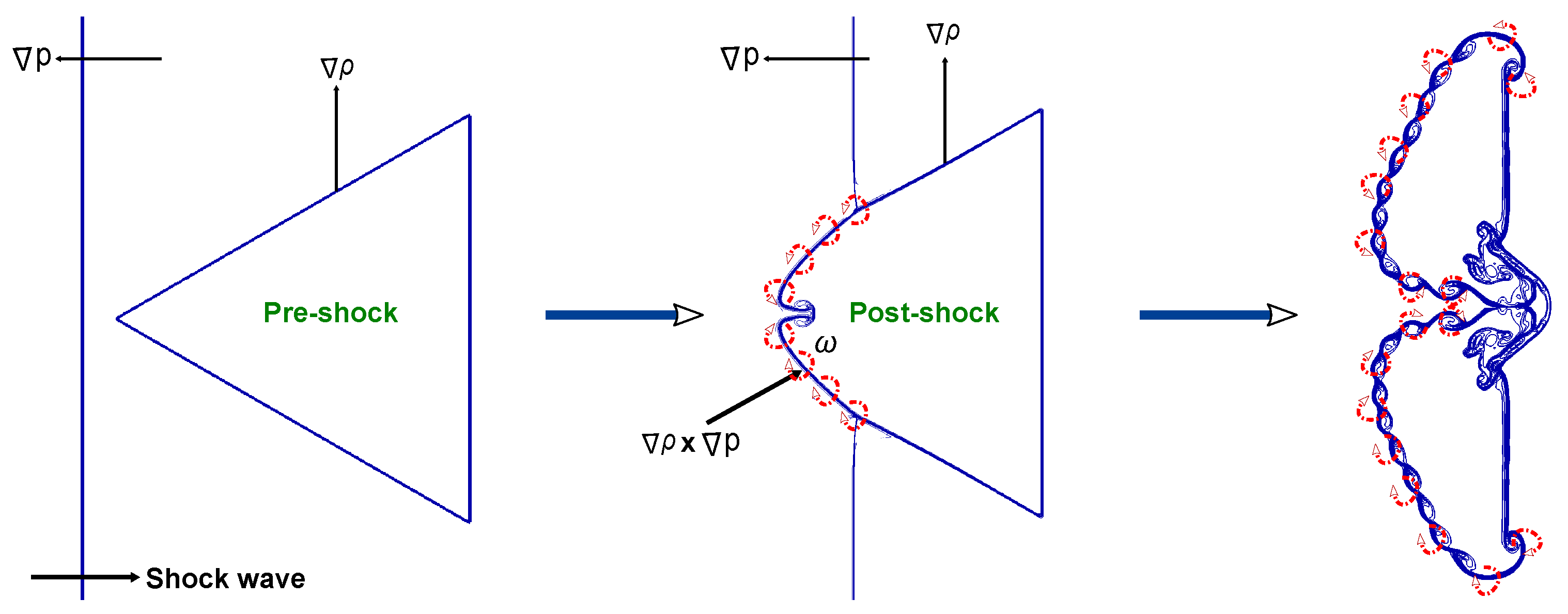
2.4.3. Vorticity Transport Equation

The vorticity transport equation for compressible Euler flows is expressed as follows:

$$\begin{array}{c}\hfill \frac{D\omega }{D\tau }=(\omega ·\nabla )\mathbf{u}-\omega (\nabla ·\mathbf{u})+\frac{1}{{\rho }^2}(\nabla \rho \times \nabla p).\end{array}$$

(20)

Here, the term on the left-hand side represents the material derivatives, which are comprised of the sum of the unsteady component, ${\omega }_t=\partial \omega /\partial \tau$, and the convection component, ${\omega }_c=(\mathbf{u}·\nabla )\omega$. The initial term on the right-hand side denotes vorticity stretching originating from velocity gradient variations within the flow, a phenomenon that is absent in two-dimensional turbulent flows. The subsequent term signifies vorticity stretching attributed to flow compressibility. Lastly, the third term represents baroclinic vorticity, which is crucial for generating small-scale vortical structures at the interface of the bubble.

2.4.4. Spatial Integrated Field of Vorticity Production Terms

In order to improve our comprehension of the relationship between the Atwood number’s influence and the vorticity formation in shock-induced bubbles, we analyze three important factors that are spatially integrated: mean vorticity, dilatational vorticity production, and baroclinic vorticity production terms. These spatially integrated fields are defined as

$${\omega }_{av}\left(\tau \right)=\frac{{\int }_D|\omega |dxdy}{{\int }_{D}dxdy},$$

(21)

$${\omega }_{dil}\left(\tau \right)=-\frac{{\int }_D\left|\omega (\nabla ·\mathbf{u})\right|dxdy}{{\int }_{D}dxdy},$$

(22)

$${\omega }_{bar}\left(\tau \right)=\frac{{\int }_D\left|\frac{1}{{\rho }^2}(\nabla \rho \times \nabla p)\right|dxdy}{{\int }_{D}dxdy},$$

(23)

where D represents the entire computational domain.

2.4.5. Enstrophy

Enstrophy represents the integral of vorticity squared across the flow field, which provides insight into the temporal evolution of vorticity distribution. It is defined as

$$\Omega \left(\tau \right)=\frac{1}{2}{\int }_D{\omega }^{2}dxdy.$$

(24)

2.4.6. Kinetic Energy

The spatial integral of the square of the velocity vector in the flow field represents the time development of the kinetic energy (K.E.), which is defined as

$$\mathrm{K}.\mathrm{E}.\left(\tau \right)=\frac{1}{2}{\int }_D{\mathbf{u}}^{2}dxdy.$$

(25)

3. Problem Setup and Grid Refinement Study

3.1. Problem Setup

Figure 2 depicts a schematic representation of the problem configuration involving a shock-induced forward-triangular bubble. A rectangular domain measuring $200\mathrm{mm}\times 100\mathrm{mm}$ is utilized for conducting the numerical simulations. The setup comprises a moving planar shock wave and a stationary forward-triangular bubble filled with light gas. The planar shock wave, characterized by three Mach numbers ${\mathrm{M}}_s=1.12,1.21,1.41$, propagates from left to right along the x-direction. Positioned at a distance of 5 mm from the shock wave’s origin, the triangular bubble’s initial location is 20 mm from the left boundary of the domain. The forward-triangular bubble features a fixed edge length of $L=30$ mm in this arrangement. In the computational domain, the left boundary serves as an inflow boundary, while the upper, bottom, and right boundaries are designated as outlets. The primary focus of this initial setup is the investigation of the RM phenomena in forward-triangular light gas bubbles under varying Atwood numbers. Therefore, the initial pressure and temperature surrounding the triangular bubble are specified as $P_0=101,325$ Pa and $T_0=273$ K, respectively. Three different light gases—neon (Ne), helium (He), and hydrogen (H₂)—are considered for the forward-triangular bubbles, while nitrogen is selected as the ambient gas. The physical properties of these gases are summarized in

Table 1. Gas parameters for the numerical simulations at $P_0=101,325$ Pa and $T_0=293$ K.

Gas	Density	Heat Ratio	Sound Speed	Atwood Number
	$(\mathit{\rho },\mathbf{kg}·{\mathbf{m}}^{-\mathbf{3}})$	($\mathit{\gamma }$)	$(\mathit{c},\mathbf{m}·{\mathbf{s}}^{-\mathbf{1}})$	(At)
${\mathrm{N}}_2$	1.25	1.40	352	ambient
Ne	0.80	1.03	452	−0.218
He	0.16	1.66	1007	−0.773
${\mathrm{H}}_2$	0.084	1.41	1320	−0.874

.

3.2. Initialization of Numerical Simulations

To commence the numerical simulations, we establish an ambient condition on the right side of the shock wave. Utilizing the classical Rankine–Hugoniot conditions, we derive the primitive variables on the left side of the shock wave. The classical Rankine–Hugoniot conditions for computations employing primitive variables are articulated as

$${\mathrm{M}}_2^2=\frac{1+\left[\frac{(\gamma -1)}{2}\right]{\mathrm{M}}_s^2}{\gamma {\mathrm{M}}_s^2-\frac{(\gamma -1)}{2}},\frac{p_2}{p_1}=\frac{1+\gamma {\mathrm{M}}_s^2}{1+\gamma {\mathrm{M}}_2^2},\frac{{\rho }_2}{{\rho }_1}=\frac{\gamma -1+(\gamma +1)\frac{p_2}{p_1}}{\gamma +1+(\gamma -1)\frac{p_2}{p_1}}.$$

(26)

Here, ${\mathrm{M}}_s$ denotes the Mach number of the shock, while the subscripts 1 and 2 correspond to the left and right sides of the shock wave, respectively.

In the subsequent simulations, normalized time is employed to present snapshots of the flow morphology. The actual computational time is normalized by the characteristic time $t_0=L/W_i$, where $\tau =t/t_0=t{W}_i/L$, with $W_i$ representing the velocity of the incident shock wave and L denoting the edge length of the square. For visualization of the numerical outcomes, numerical shadowgraphs are utilized, which rely on the density gradient magnitude, denoted as $s=|\nabla \rho |$.

3.3. Grid Refinement Study

To ensure accuracy and efficiency in simulating the Richtmyer–Meshkov (RM) instability, a grid sensitivity analysis is conducted. This involves a test case featuring a shock-induced forward-triangular bubble filled with helium, surrounded by nitrogen gas, utilizing four different grid sizes labeled ‘Grid-1’ through ‘Grid-4’, corresponding to grid points of $200\times 100$, $400\times 200$, $800\times 400$, and $1200\times 600$, respectively. Figure 3 displays numerical shadowgraphs at $\tau =15$ for these varying grid resolutions. As seen in the figure, higher grid resolution results in a sharper interface and improved clarity of discontinuities, including interface and shock discontinuities. Grid size $1200\times 600$ effectively captures small-scale rolled-up vortices. Furthermore, density profiles along the centerline at these four grid resolutions are shown in Figure 3 to illustrate grid sensitivity. The results indicate a decrease in density dissipation with increasing grid resolution. Consequently, grid resolutions of $1200\times 600$ are chosen for all computational simulations based on these observations.

4. Results and Discussion

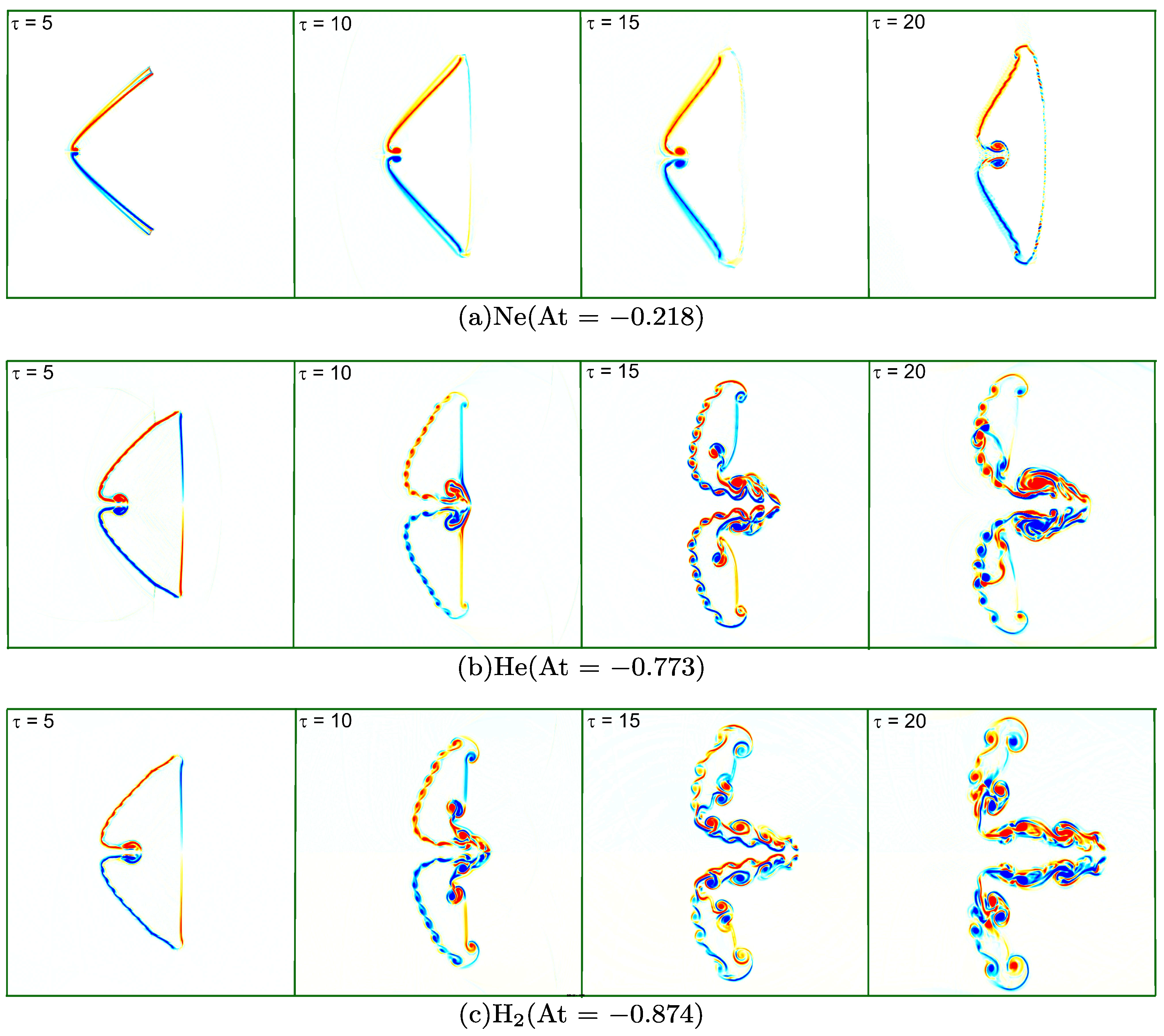
4.1. Evolution of Flow Morphology

An essential aspect of RM instability is observing the evolution of flow morphology. Therefore, Figure 4, Figure 5 and Figure 6 depict the evolution of flow morphology for shock-induced forward-triangular bubbles filled with various light gases and having different Atwood numbers at ${\mathrm{M}}_s=1.21$. In these simulations, the triangular bubbles are filled with neon, helium, or hydrogen gas, while the surrounding gas is nitrogen. As a result, the shocked forward-triangular light gas bubbles exhibit negative Atwood numbers, indicating a “slow-fast” or “divergent” configuration of the flow field.

Figure 4 presents a detailed evolution of flow morphology for the shock-induced forward-triangular Ne bubble with $\mathrm{At}=-0.218$ at ${\mathrm{M}}_s=1.21$. Each sub-figure depicts mass fraction contours in the upper half and numerical shadowgraphs in the lower half. Upon interaction of the incident shock (IS) wave with the leading edge of the forward-triangular bubble, a first transmitted shock (TS) wave propagates downwards within the neon bubble, while a curved reflected shock (CRS) wave moves upwards in the surrounding ambient gas ($\tau =1$). The TS wave travels faster inside the bubble compared to the ambient gas due to the slightly lower acoustic impedance of Ne gas. An inward nitrogen jet (IJ) forms at the leading edge of the triangular bubble as nitrogen gas penetrates into the Ne bubble following the IS wave interaction ($\tau =2$). Over time, an irregular pattern emerges, featuring a triple point (TP) and a Mach stem (MS) outside the bubble ($\tau =5$). Interestingly, no free precursor shock wave is observed in this scenario. As time progresses, the TS wave reaches the downstream interface inside the bubble, resulting in the simultaneous formation of a second transmitted shock (STS) traveling downwards and a reflected transmitted shock (RTS) wave moving upwards ($\tau =7$). As the interaction continues, the neon triangular bubble begins to compress, and the rightmost corners of the triangular bubble gradually flex due to baroclinic vorticity ($\tau =150$). Notably, two small jet-associated vortices (JAV) appear at the leftmost side of the forward-triangular bubble, gradually penetrating and causing the triangular bubble to collapse. With further progression, the middle corners of the bubble become increasingly twisted inward, and the rear corners of the surface gradually bend ($\tau$ = 15–25).

Figure 5 depicts the evolution of flow morphology for the shock-induced forward-triangular helium bubble with $\mathrm{At}=-0.773$ at ${\mathrm{M}}_s=1.21$. Upon interaction of the IS wave with the forward-triangular bubble, a transmitted shock TS propagates downwards within the bubble, while a curved reflected shock CRS, accompanied by a reflected rarefaction wave (RRW), moves upwards in the surrounding nitrogen gas. Due to the low density of the helium triangular bubble, the TS wave moves significantly faster over the interface compared to the IS wave from the outside. Unlike neon gas, the inward jet (IJ) that forms at the leading edge of the helium triangular bubble penetrates deeply. Subsequently, the TS wave generates a new oblique shock wave in the surrounding gas, known as the free precursor shock (FPS), after refraction at the triangular interface ($\tau =3$). This leads to the formation of an irregular refraction wave pattern, including a Mach stem (MS) and a triple point (TP) outside the triangle, referred to as “twin von Neumann refraction” (TNR) ($\tau =5$). Additionally, due to vorticity deposition, two small vortices become visible at the right corners of the triangular bubble ($\tau =7$). As time progresses, the TS wave interacts with the downstream interface inside the pentagon, resulting in the creation of an upward-moving reflected transmitted shock (RTS) wave and a downward-moving second transmitted shock (STS) in the flow field. The interaction between the IS wave and the triangular bubble continues over time, leading to the presence of a detached shock (DS) wave along the rightmost interface. Moreover, the RTS wave inside the bubble moves upwards and collides with the upstream interface. The evolution of the flow field is gradually less affected by the IS wave over time, and vortex rings at the right corners grow due to vorticity production. Additionally, Kelvin–Helmholtz instability leads to the emergence of small-scale vortex formations on the deformed triangular interface. Notably, two distinct trailing bubbles (TB) appear at the right corners of the bubble, potentially resulting from large-scale RM instability. Interestingly, the size of the jet-associated vortices JAV increases over time due to enhanced compression effects. As the jet emerges with the downstream interface, the formed triangular bubble divides into two symmetrical vortex rings (PV, SV1) connected by a bridge CB and line CL. Ultimately, the deformation of the triangular bubble becomes increasingly complex, with the resulting flow field primarily governed by the formed vortex rings at later stages.

Figure 6 illustrates the evolution of flow morphology for the shock-induced forward-triangular ${\mathrm{H}}_2$ bubble with $\mathrm{At}=-0.874$ at ${\mathrm{M}}_s=1.21$. Similar to the forward-triangular helium bubble, complex wave patterns (CRW, RRW, TS, STS, FPS, RTS, etc.), TNR reflection pattern (TP, MS), primary vortex ring (PVR), and trailing bubble (TB) are observed in the flow field. Additionally, a re-entrant jet (IJ) forms in the middle of the upstream interface due to the influence of ambient gas driven by generated vorticity. The early-stage interface morphology progression of the ${\mathrm{H}}_2$ bubble is identical to that of the helium bubble, as observed in Figure 5. Interestingly, three types of secondary vortex rings (SV1, SV2, SV3) emerge in the flow fields, gradually dispersing and enlarging, leading to bubble collapse. This type of vortex formation is not observed in the other light gas bubbles. At later stages, the developed vortex rings entirely dictate the flow field and facilitate turbulent mixing of ambient and bubble gases.

Figure 7 illustrates the Atwood number impact on interface deformation within shock-induced forward-triangular light bubbles. The bubble experiences compression along the x-direction induced by the IS wave, causing its leading edges to advance closer to the horizontal axis of symmetry compared to the middle section. This compression initiates upon the arrival of the IS wave at the upstream end of the bubble during the initial interaction. Across all three Atwood numbers, both the upstream and downstream interfaces swiftly propagate, with the upstream side inwardly pressed by the IS wave in the early stages, as depicted in Figure 7a–c. As time progresses, two small vortices form at the right corners of the triangular interface due to vorticity deposition. The impact of the IS wave on interface evolution leads to the gradual growth of the vortex pair at the corners. Subsequently, both the upper and lower interfaces of the bubble fold inward toward the upstream axis, resulting in a divergent shape. Notably, at $\mathrm{At}=-0.218$, the size of rolled-up vortices is comparatively smaller than at higher negative Atwood numbers, with these vortices continuously enlarging over time. At later stages, the flow field is predominantly influenced by the rolled-up vortices. Remarkably, the length of the deformed triangular interface is greater at $\mathrm{At}=-0.874$.

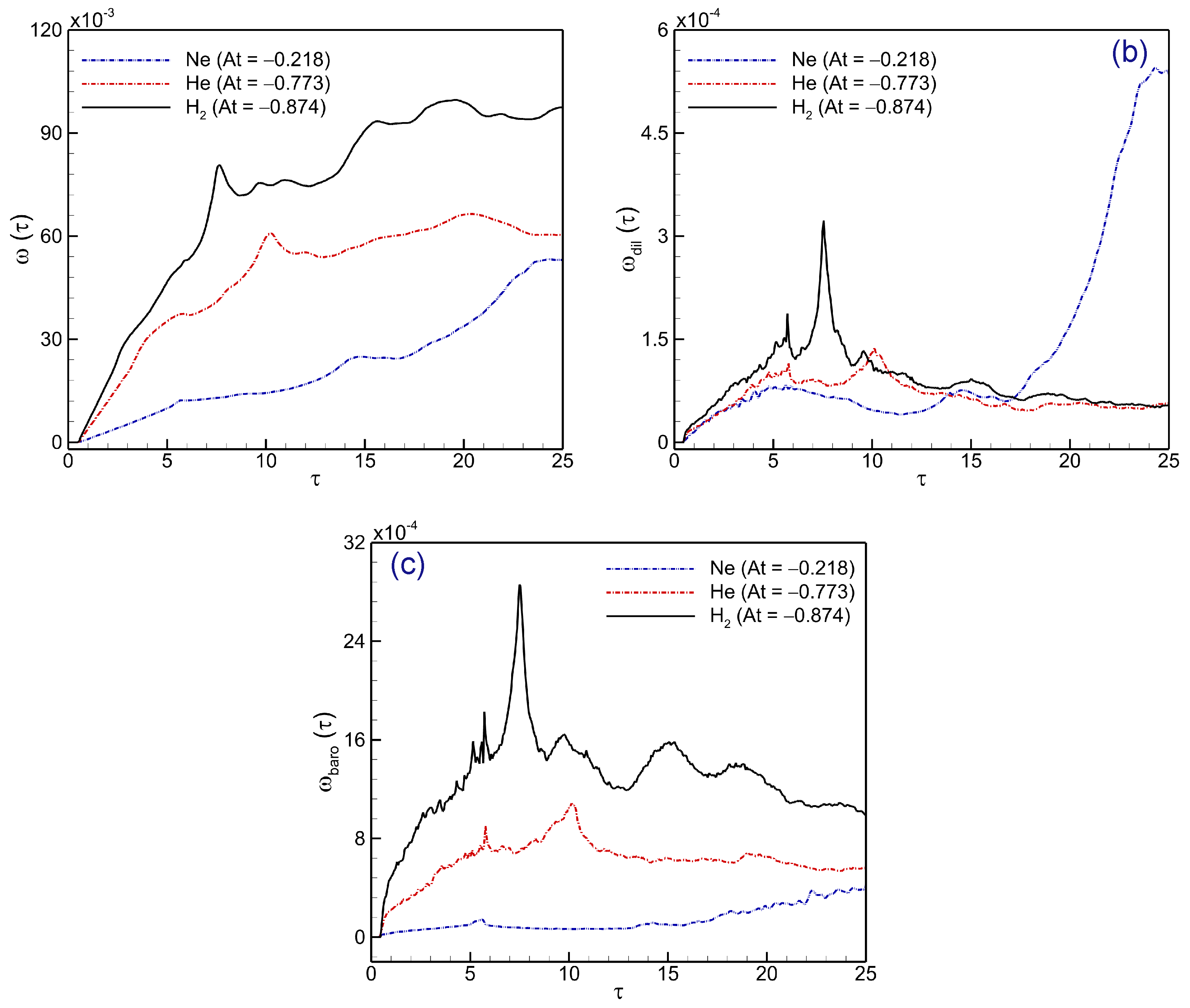
4.2. Vorticity Generation

The accumulation of baroclinic vorticity along the bubble interface plays a significant role in the development of RM phenomena. In this analysis, we aim to explore in detail how the baroclinic vorticity term influences both incident and transmitted shock waves during the initial stages of their interaction with a stationary triangular bubble interface. Figure 8 provides a visual representation illustrating the process of vorticity formation on the forward-triangular interface following the passage of the initial shock wave. In the context of shock-induced bubble flow, the shock wave typically imposes a predominant pressure gradient, whereas the bubble interface exhibits a dominant density gradient. As the shock wave passes over the bubble, it generally induces minimal changes to the bubble itself. However, when the shock wave reaches the upper and lower corners of the leftmost vertical interface, where pressure and density gradients align perfectly, a small amount of vorticity, or rolled-up vortex, is generated. Mach reflection occurs as the shock progresses along the inclined interfaces, leading to the merging of the Mach stem with the incident shock wave and the triangular interface. Consequently, as the shock wave traverses over the triangular bubble and moves upward, the Mach stem imparts the necessary pressure gradient required to initiate vorticity on the interface, gradually triggering the baroclinic vorticity term.

Figure 9 demonstrates how the Atwood number influences vorticity distribution in shock-induced forward-triangular bubbles at different time intervals. Initially, vorticity is uniformly zero across the domain. Upon interaction with the IS wave, baroclinic vorticity is primarily localized at the bubble interface, especially where there is a disparity between the bubble gas and the surrounding ambient gas. At points where density and pressure gradients are perpendicular, such as the top and bottom of the bubble, vorticity reaches its maximum, while it remains zero along the interface axis where these gradients align. Notably, substantial positive vorticity accumulates on the upper part of the bubble interface, while significant negative vorticity forms on the lower horizontal side, due to the IS wave propagating from left to right along the interface. The vortical structure at the upper interface exhibits positive vorticity at the center, surrounded by negative vorticity tails, with the opposite pattern observed at the bottom interface. Following the interaction, noticeable differences in vorticity distribution are observed for the three Atwood numbers. $\mathrm{At}=-0.218$, only a small amount of vorticity is evident at the rolled-up vortices on the bubble interface, whereas at $\mathrm{At}=-0.773$ and $\mathrm{At}=-0.874$, the rolled-up vortices are more pronounced. Consequently, vorticity generation and distribution play a crucial role, especially at the largest negative Atwood numbers, when rolled-up vortices are prominent.

To enhance our understanding of how the Atwood number affects vorticity formation in shock-induced forward-triangular light bubbles, we examine the spatially integrated fields of average vorticity, dilatational and baroclinic vorticity production terms. Figure 10 demonstrates the influence of the Atwood number on the spatially integrated characteristics of mean vorticity, as well as dilatational and baroclinic vorticity production terms in shock-induced forward-triangular light bubbles. It is evident that these integrated quantities are at their smallest levels for $\mathrm{At}=-0.218$ among the three Atwood numbers when the incident and reflected shock waves interact with the bubble. Conversely, these integrated quantities are notably amplified for $\mathrm{At}=-0.874$. Across all Atwood numbers, these integrated quantities exhibit a rise over time, indicating an increasing entrainment of ambient gas into the distorted forward-triangular light gas bubbles. Upon the impact of the incident and reflected shock waves on the bubbles, the mean vorticity value increases, facilitating the mixing of gases both inside and outside the bubble, thereby accelerating energy transmission and consumption, as shown in Figure 10a. Consequently, this may lead to a gradual reduction in mean vorticity intensity within the bubble region. Notably, both vorticity production terms attain significant values during the interaction. The plot of the dilatational vorticity production term depicts locally stretched structures around the vortex core due to compressibility effects arising from localized regions of compression and expansion, as illustrated in Figure 10b. Meanwhile, the plot of the baroclinic vorticity production term illustrates the misalignment of pressure and density gradients, which in turn, generates vorticity due to the presence of contact discontinuity and reflected shock structures, as seen in Figure 10c. The vortices generated by the interaction between the shock wave and the bubble promote the mixing of ambient gas with the forward-triangular light gas bubbles. Upon the subsequent impingement of reflected shock waves on the distorted bubble, the spatially integrated quantities exhibit their highest growth rates, indicating a significant enhancement in vorticity during this phase. Subsequently, the growth rate in the flow field slows down.

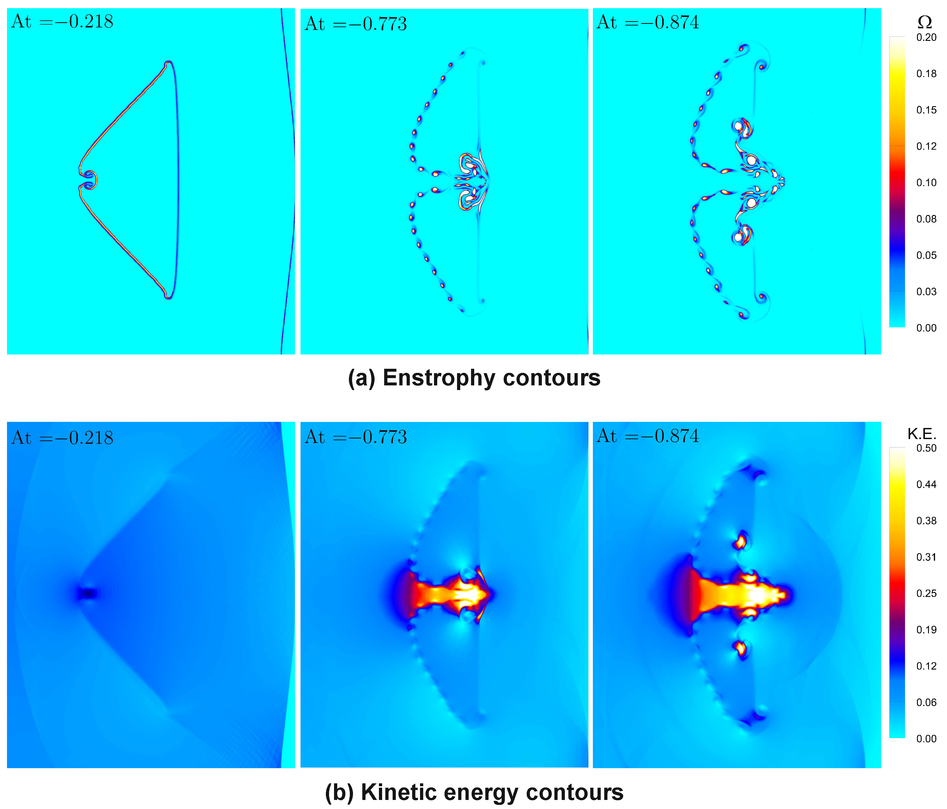
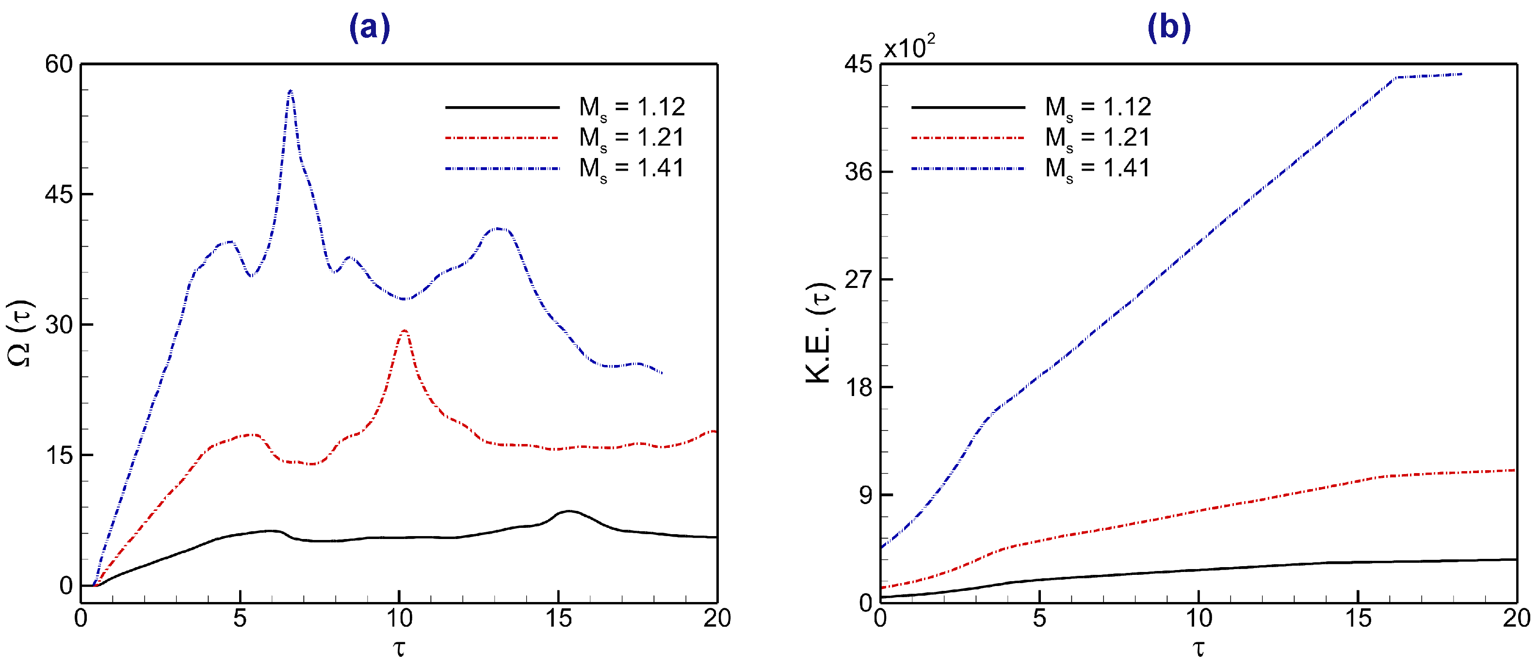
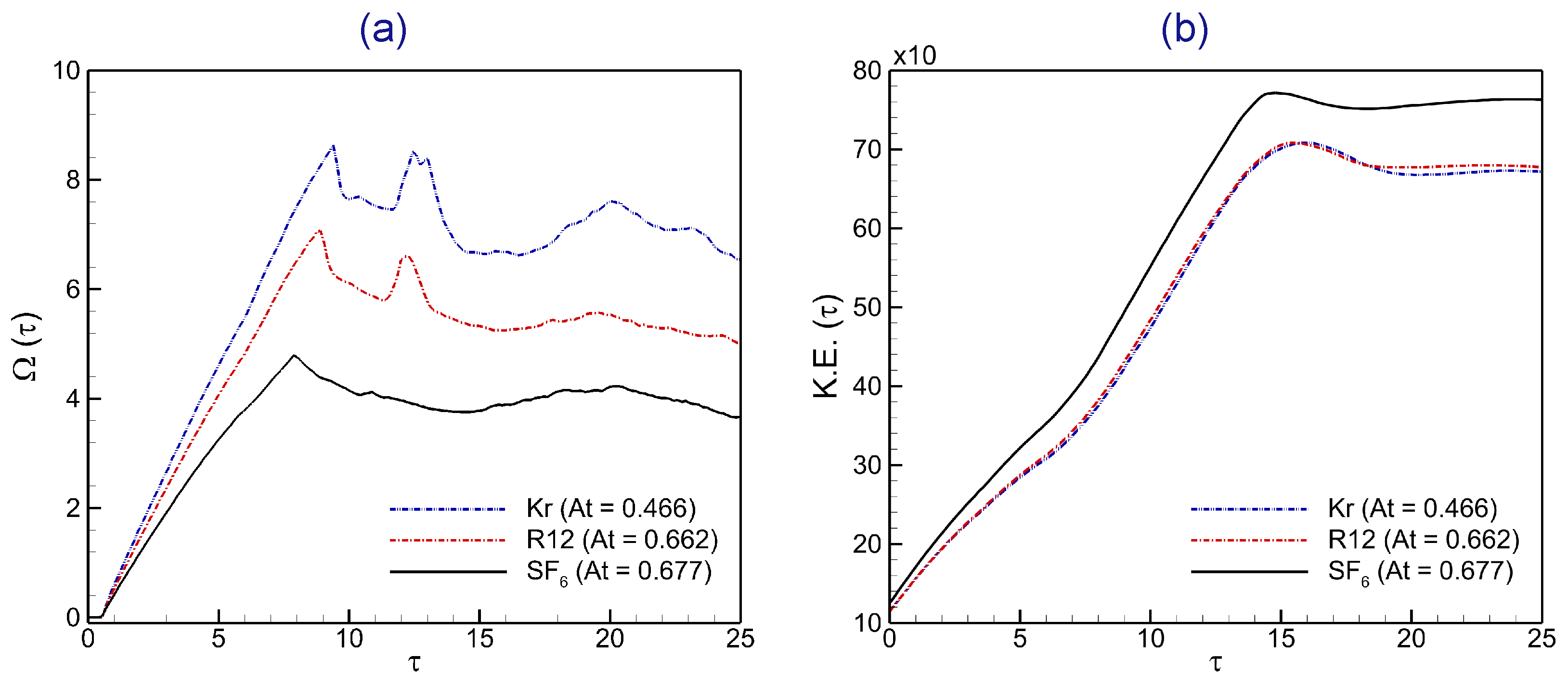
4.3. Evolution of Enstrophy and Kinetic Energy

To further explore the Atwood number impact on the physical processes associated with shock-induced forward-triangular bubbles, we discuss here the evolution of enstrophy and kinetic energy.

Figure 11 illustrates the Atwood number impacts on the contours of enstrophy ($\Omega$) and kinetic energy (K.E.) in shock-induced forward-triangular light gas bubbles at $\tau =10$. Post-interaction, notable disparities in enstrophy and kinetic energy are observed across various Atwood numbers. Additionally, substantial amounts of enstrophy and kinetic energy are observed within the rolled-up vortex rings of the deformed bubble interface. Particularly at $\mathrm{At}=-0.874$, the flow fields of these quantities exhibit significant enhancement compared to $\mathrm{At}=-0.218$. To further explore the influence of the Atwood number, spatial integrated fields of enstrophy and kinetic energy over time are presented in Figure 12. Enstrophy remains at zero until the shock wave reaches the upstream interface of the triangular bubble, after which the creation of baroclinic vorticity leads to an increase. Enstrophy rises notably at the bubble interface where the shock and reflected shock waves impinge. The heightened vorticities then facilitate the mixing of gases within and outside the bubble, expediting energy transfer and consumption, which could gradually diminish the enstrophy intensity within the bubble zone. This phenomenon is observed across all Atwood numbers, with only the total enstrophy levels differing due to the generation of more enstrophy by ${\mathrm{H}}_2$ gas. Conversely, the evolution of kinetic energy, as depicted in Figure 12b, exhibits variations dependent on gas properties, with a notable increase observed at $\mathrm{At}=-0.874$.

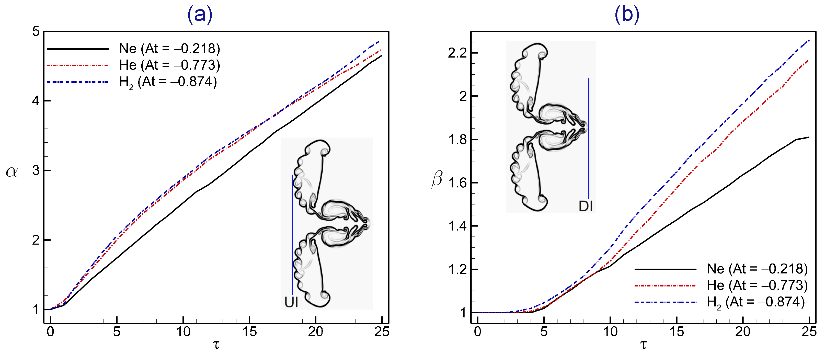
4.4. Interface Features

In this section, we conduct a quantitative analysis of the interface characteristics of shock-driven forward-triangular light gas bubbles to elucidate the effects of the Atwood number. The interface features of the triangular bubble include the displacement of the upstream interface (UI), downstream interface (DI), interface width $\left(w\right)$ in the x-direction, and interface height $\left(h\right)$ in the y-direction.

Figure 13 depicts how the Atwood number influences the temporal changes in the normalized distances upstream ($\alpha$) and downstream ($\beta$) of the forward-triangular bubble following impingement by the IS wave. These normalized distances are calculated as $\alpha =\mathrm{UI}/d_{\mathrm{UI}}$ and $\beta =\mathrm{DI}/d_{\mathrm{DI}}$, where $d_{\mathrm{UI}}$ and $d_{\mathrm{DI}}$ represent the original distances of UI and DI positions from the IS wave, respectively. In Figure 13a, it is evident that $\alpha$ exhibits similar behavior at early stages for all three Atwood numbers in the forward-triangular bubble. Subsequently, it accelerates, likely due to the production of rarefaction waves when the shock wave interacts with the downstream contact. Strong compression effects lead to increased $\alpha$ values at higher negative Atwood numbers for the triangular bubble interface. Observations suggest that the displacement of $\alpha$ is greater in ${\mathrm{H}}_2$ gas and diminishes in Ne gas. Conversely, during the initial phase, the $\beta$ value of forward-triangular bubbles remains stationary until encountering the STS wave, as depicted in Figure 13b. Once the STS wave dissipates, $\beta$ achieves a certain velocity, initiating the acceleration of various vortex rings. Notably, displacement in $\beta$ is observed at a higher level of $\mathrm{At}=-0.874$.

Figure 14 illustrates the Atwood number impacts on temporal variations of the normalized interface width and height for the computed shock-induced forward-triangular light gas bubble. These normalized quantities are defined as $w^{*}=(w-w0)/w_0$ and $h^{*}=(h-h_0)/h_0$, with the subscript ’0’ representing the initial interface value. Initially, the width of the evolving interface experiences rapid reduction during the early stages of interaction due to compression induced by the passage of the IS wave, as depicted in Figure 14a. After the compression phase, Ne gas ($\mathrm{At}=-0.218$) demonstrates a gradual decrease in the temporal variation of width, while He and ${\mathrm{H}}_2$ gases ($\mathrm{At}=-0.773$ and $-0.874$) exhibit rapid growth in the temporal variation of length due to the intensified formation of rolled-up vortices. Notably, the increasing heights of the evolving interface result from the continued rotation of vortex pairs until the interface is impacted by reflected shock waves, which diminish the rate of interface height development, as illustrated in Figure 14b. The maximum and minimum heights of the developing interface are observed at $\mathrm{At}=-0.874$ and $-0.218$, respectively.

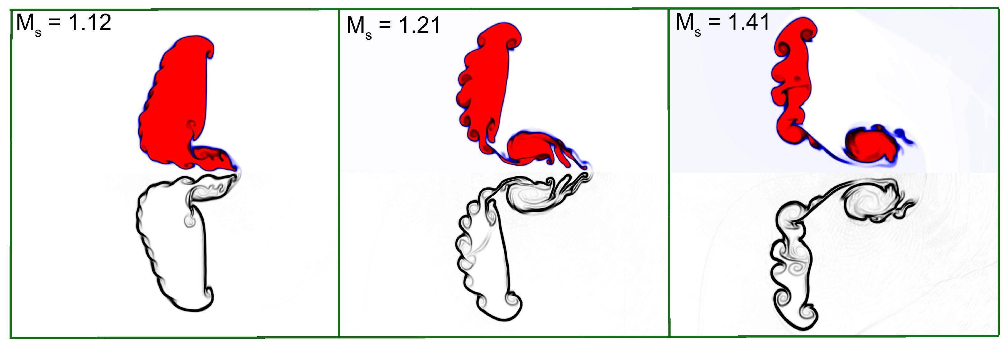
4.5. Impact of Shock Mach Number

In this section, we analyze the impact of shock Mach numbers on shock-driven forward-triangular light gas bubbles. Figure 15 depicts the effects of three shock Mach numbers (${\mathrm{M}}_s=1.12,1.21,1.41$) on the flow morphology of shock-driven forward-triangular bubbles containing helium gas. It is evident that higher shock Mach numbers result in a more intense interaction between the shock wave and the bubble. The height of the generated jet increases as the strength of the incident shock wave rises, owing to the upward expansion of the bubble interface. Moreover, with increasing Mach numbers, the bubble undergoes significant deformation, leading to more intricate wave patterns and noticeable reductions in bubble size. Additionally, at higher shock Mach numbers, the size and intensity of the rolled-up vortices notably increase, becoming prominent at the interface between the bubbles and the surrounding gas due to the deposition of baroclinic vorticity.

Figure 16 demonstrates the effects of shock Mach numbers on the spatially integrated fields of enstrophy and kinetic energy in shock-induced forward-triangular helium bubbles. It is evident that at $\mathrm{M}s=1.12$, these integrated fields are the smallest among the three shock Mach numbers when the incident and reflected shock waves interact with the double bubble. Conversely, both integrated fields are significantly amplified in the case of $\mathrm{M}s=1.41$. Over time, the spatially integrated fields for each of the three Mach numbers exhibit a gradual increase, indicating that the distorted forward-triangular helium bubbles increasingly incorporate the surrounding ambient gas. In summary, the flow morphology of forward-triangular light gas bubbles becomes more pronounced as the shock Mach number increases.

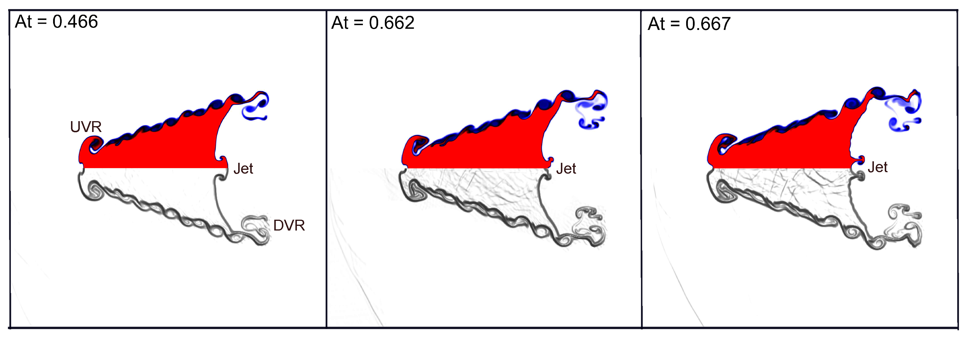
4.6. Impact of Positive Atwood Number

Finally, this section briefly discusses the effects of a positive Atwood number on shock-induced forward-triangular heavy bubbles. When the bubble density is greater than the density of the surrounding gas, the value of the Atwood number becomes positive, i.e., $\mathrm{At}>0$, and this scenario represents the “fast-slow” or “heavy-light” configuration. To this end, we examine three distinct heavy gases—Kr, R12, and ${\mathrm{SF}}_6$—which result in positive Atwood numbers of $\mathrm{At}=0.466$, $0.662$, and $0.677$, respectively. In these cases, due to the higher acoustic impedance $(Z=\rho c)$ within the bubbles, the shock wave propagates more slowly inside than outside [49]. Consequently, the transmitted shock waves inside the forward-triangular bubbles lag significantly behind the incident shock wave outside the bubbles. Notably, the flow structures produced and the associated RM instability exhibit notable differences when $\mathrm{At}>0$ compared to when $\mathrm{At}<0$.

Figure 17 illustrates the effects of positive Atwood number ($\mathrm{At}=0.466$, $0.662$, and $0.677$) on the flow morphology of shock-driven forward-triangular heavy bubbles with ${\mathrm{M}}_s=1.21$ at time $\tau =20$. In all three cases, upstream and downstream vortex rings (UVR and DVR) are generated in the flow field during the interaction process. Additionally, various types of outward jets are observed near the downstream centerlines due to propelling by the peak pressure created by the complex interaction of shocks inside the bubble. Furthermore, the moderate size of the KH instability, characterized by rolled-up vortices increases, making them more prominent at the bubble-gas interface. Over time, the resulting outward jet expands along both vortex pairs, UVR and DVR. Figure 18 shows the positive Atwood number impacts on the spatial integrated fields of enstrophy and kinetic energy in shock-induced forward-triangular heavy bubbles. It can be observed that as the positive Atwood number increases, the spatially integrated values of enstrophy decrease, while the spatially integrated values of kinetic energy increase.

5. Concluding Remarks and Outlook

In this study, we have conducted a numerical investigation aimed at unraveling the intricate dynamics of Richtmyer–Meshkov (RM) phenomena initiated by the interaction of shock waves with forward-triangular light gas bubbles. The triangular bubbles, filled with neon, helium, or hydrogen gas and surrounded by nitrogen gas were subjected to three different shock Mach numbers: ${\mathrm{M}}_s=1.12,1.21,$ and 1.41. Utilizing a two-dimensional system of compressible Euler equations for two-component gas flows, we employed a high-fidelity explicit modal discontinuous Galerkin technique for numerical simulations. Our numerical results were validated against existing experimental data, demonstrating good agreement.

The numerical findings underscore the pivotal role of the Atwood number in dictating the growth of RM instability within shock-induced forward-triangle light bubbles. Variations in the Atwood number exert profound effects on flow morphology, leading to the emergence of intricate wave patterns, the formation of inward jets, bubble deformation, and the generation of vorticity. Interestingly, it is observed that alterations in the Atwood number result in distinct deformations of the bubble. Moreover, higher Atwood numbers are associated with the production of larger chains of rolled-up vortices compared to lower Atwood numbers. A comprehensive examination of the effects of the Atwood number is further presented to elucidate the driving mechanisms behind vorticity formation during the interaction process. Notably, vorticity emerges as a crucial factor in elucidating the key features of the forward-triangular bubble. It is noted that vorticity within the bubble region intensifies with increasing Atwood numbers, accompanied by a significant rise in enstrophy and kinetic energy. Additionally, the impacts of the Atwood number on temporal variations in interface features are thoroughly explored. Finally, the influence of the shock Mach numbers and positive Atwood numbers on shock-induced forward-triangular bubbles is investigated.

The primary objective of this study was to explore how the Atwood number influences RM instability within forward-triangular light gas bubbles. It is noteworthy that the interaction between a planar shock wave and polygonal bubbles with re-shock could potentially have significant implications for the evolution of RM instability. Consequently, it is anticipated that future research endeavors will expand upon this work to investigate RM instability in shock-induced polygonal bubbles under re-shock conditions.

References

1. Richtmyer, R.D. Taylor instability in shock acceleration of compressible fluids. Commun. Pure. Appl. Math. 1960, 13, 297–319. [Google Scholar] [CrossRef]
2. Meshkov, E.E. Instability of the interface of two gases accelerated by a shock wave. Fluid Dyn. 1969, 4, 101. [Google Scholar] [CrossRef]
3. von Helmholtz, H. Über Discontinuirliche Flüssigkeits-Bewegungen; Akademie der Wissenschaften zu Berlin: Berlin, Germany, 1868. [Google Scholar]
4. Kelvin, L. On the motion of free solids through a liquid. Phil. Mag. 1871, 42, 362–377. [Google Scholar]
5. Arnett, W.D.; Bahcall, J.N.; Kirshner, R.P.; Woosley, S.E. Supernova 1987A. Ann. Rev. Astron. Astrophys. 1989, 2, 629–700. [Google Scholar] [CrossRef]
6. Lindl, J.; Landen, O.; Edwards, J.; Moses, E.; Team, N. Review of the national ignition campaign 2009–2012. Phys. Plasmas 2014, 21, 020501. [Google Scholar] [CrossRef]
7. Yang, J.; Kubota, T.; Zukoski, E.E. Applications of shock-induced mixing to supersonic combustion. AIAA J. 1993, 31, 854–862. [Google Scholar] [CrossRef]
8. Zeng, W.G.; Pan, J.H.; Sun, Y.T.; Ren, Y.X. Turbulent mixing and energy transfer of reshocked heavy gas curtain. Phys. Fluids 2021, 30, 064106. [Google Scholar] [CrossRef]
9. Brouillette, M. The Richtmyer–Meshkov instability. Annu. Rev. Fluid Mech. 2002, 34, 445. [Google Scholar] [CrossRef]
10. Zhou, Y. Rayleigh–Taylor and Richtmyer–Meshkov instability induced flow, turbulence, and mixing. I. Phys. Rep. 2017, 720, 1–136. [Google Scholar]
11. Zhou, Y. Rayleigh–Taylor and Richtmyer–Meshkov instability induced flow, turbulence, and mixing. II. Phys. Rep. 2017, 723, 1–160. [Google Scholar]
12. Zhou, Y.; Williams, R.J.; Ramaprabhu, P.; Groom, M.; Thornber, B.; Hillier, A.; Mostert, W.; Rollin, B.; Balachandar, S.; Powell, P.D.; et al. Rayleigh–Taylor and Richtmyer–Meshkov instabilities: A journey through scales. Physica D 2021, 423, 132838. [Google Scholar] [CrossRef]
13. Jahn, R.G. The refraction of shock waves at a gaseous interface. J. Fluid Mech. 1956, 1, 457–489. [Google Scholar] [CrossRef]
14. Abd-El-Fattah, A.M.; Henderson, L.F. Shock waves at a fast-slow gas interface. J. Fluid Mech. 1978, 86, 15–32. [Google Scholar] [CrossRef]
15. Henderson, L.F. The refraction of a plane shock wave at a gas interface. J. Fluid Mech. 1966, 26, 607–637. [Google Scholar] [CrossRef]
16. Abd-El-Fattah, A.M.; Henderson, L.F. Shock waves at a slow-fast gas interface. J. Fluid Mech. 1978, 89, 79–95. [Google Scholar] [CrossRef]
17. Abd-El-Fattah, A.M.; Henderson, L.F.; Lozzi, A. Precursor shock waves at a slow—Fast gas interface. J. Fluid Mech. 1976, 76, 157. [Google Scholar] [CrossRef]
18. Henderson, L.F.; Colella, P.; Puckett, E.G. On the refraction of shock waves at a slow—Fast gas interface. J. Fluid Mech. 1991, 224, 1. [Google Scholar] [CrossRef]
19. Markstein, G.H. A Shock-Tube Study of Flame Front-Pressure Wave Interaction, 6th ed.; International Symposium on Combustion; Elsevier: Amsterdam, The Netherlands, 1957; Volume 6, p. 387. [Google Scholar]
20. Haas, J.F.; Sturtevant, B. Interaction of weak shock waves with cylindrical and spherical gas inhomogeneities. J. Fluid Mech. 1987, 181, 41. [Google Scholar] [CrossRef]
21. Jacobs, J.W. Shock-induced mixing of a light-gas cylinder. J. Fluid Mech. 1992, 234, 629. [Google Scholar] [CrossRef]
22. Jacobs, J.W. The dynamics of shock accelerated light and heavy gas cylinders. Phys. Fluids 1993, A5, 2239. [Google Scholar] [CrossRef]
23. Layes, G.; Jourdan, G.; Houas, L. Distortion of a spherical gaseous interface accelerated by a plane shock wave. Phys. Rev. Lett. 2003, 91, 174502. [Google Scholar] [CrossRef] [PubMed]
24. Ranjan, D.; Niederhaus, J.H.J.; Oakley, J.G.; Anderson, M.H.; Bonazza, R.; Greenough, J.A. Shock-bubble interactions: Features of divergent shock-refraction geometry observed in experiments and simulations. Phys. Fluids 2008, 20, 036101. [Google Scholar] [CrossRef]
25. Zhai, Z.; Si, T.; Luo, X.; Yang, J. On the evolution of spherical gas interfaces accelerated by a planar shock wave. Phys. Fluids 2011, 23, 084104. [Google Scholar] [CrossRef]
26. Si, T.; Zhai, Z.; Luo, X. Experimental study of Richtmyer–Meshkov instability in a cylindrical converging shock tube. Phys. Fluids 2014, 32, 343–351. [Google Scholar] [CrossRef]
27. Ding, J.; Si, T.; Chen, M.; Zhai, Z.; Lu, X.; Luo, X. On the interaction of a planar shock with a three-dimensional light gas cylinder. J. Fluid Mech. 2017, 828, 289–317. [Google Scholar] [CrossRef]
28. Quirk, J.J.; Karni, S. On the dynamics of a shock-bubble interaction. J. Fluid Mech. 1996, 318, 129. [Google Scholar] [CrossRef]
29. Giordano, J.; Burtschell, Y. Richtmyer–Meshkov instability induced by shock-bubble interaction: Numerical and analytical studies with experimental validation. Phys. Fluids 2006, 18, 036102. [Google Scholar] [CrossRef]
30. Bagabir, A.; Drikakis, D. Mach number effects on shock-bubble interaction. Shock Waves 2001, 11, 209. [Google Scholar] [CrossRef]
31. Niederhaus, J.H.J.; Greenough, J.A.; Oakley, J.G.; Ranjan, D.; Anderson, M.H.; Bonazza, R.A. A computational parameter study for the three-dimensional shock-bubble interaction. J. Fluid Mech. 2008, 594, 85. [Google Scholar] [CrossRef]
32. Wang, Z.; Yu, B.; Chen, H.; Zhang, B.; Liu, H. Scaling vortex breakdown mechanism based on viscous effect in shock cylindrical bubble interaction. Phys. Fluids 2018, 30, 126103. [Google Scholar] [CrossRef]
33. Singh, S.; Battiato, M. Behavior of a shock-accelerated heavy cylindrical bubble under nonequilibrium conditions of diatomic and polyatomic gases. Phys. Rev. Fluids 2021, 6, 044001. [Google Scholar] [CrossRef]
34. Singh, S.; Battiato, M.; Myong, R.S. Impact of the bulk viscosity on flow morphology of shock-bubble interaction in diatomic and polyatomic gases. Phys. Fluids 2021, 33, 066103. [Google Scholar] [CrossRef]
35. Bai, J.; Zou, L.; Wang, T.; Liu, K.; Huang, W.; Liu, J.; Li, P.; Tan, D.; Liu, C. Experimental and numerical study of shock-accelerated elliptic heavy gas cylinders. Phys. Rev. E 2010, 82, 056318. [Google Scholar] [CrossRef]
36. Georgievskiy, P.Y.; Levin, V.A.; Sutyrin, O.G. Interaction of a shock with elliptical gas bubbles. Shock Waves 2015, 25, 357–369. [Google Scholar] [CrossRef]
37. Zou, L.; Liao, S.; Liu, C.; Wang, Y.; Zhai, Z. Aspect ratio effect on shock-accelerated elliptic gas cylinders. Phys. Fluids 2016, 28, 036101. [Google Scholar] [CrossRef]
38. Chen, J.; Qu, F.; Wu, X.; Wang, Z.; Bai, J. Numerical study of interactions between shock waves and a circular or elliptic bubble in air medium. Phys. Fluids 2021, 33, 043301. [Google Scholar] [CrossRef]
39. Singh, S.; Sengupta, B.; Awasthi, M.K.; Vinesh, V. Insight on the flow physics of shock-driven elliptical gas inhomogeneity with different Atwood numbers. Int. J. Math. Eng. Manag. Sci. 2024, 33, 1–22. [Google Scholar] [CrossRef]
40. Singh, S.; Msmali, A.H.; Nelson, M.I. Unfolding of shocked hydrodynamic instability at SF6 elliptical interface: Physical insights from numerical simulations. Comput. Fluids 2024, 277, 106304. [Google Scholar] [CrossRef]
41. Zhai, Z.; Wang, M.; Si, T.; Luo, X. On the interaction of a planar shock with a light polygonal interface. J. Fluid Mech. 2014, 757, 800–816. [Google Scholar] [CrossRef]
42. Luo, X.; Wang, M.; Si, T.; Zhai, Z. On the interaction of a planar shock with an SF6 polygon. J. Fluid Mech. 2015, 773, 366–394. [Google Scholar] [CrossRef]
43. Igra, D.; Igra, O. Numerical investigation of the interaction between a planar shock wave with square and triangular bubbles containing different gases. Phys. Fluids 2018, 30, 056104. [Google Scholar] [CrossRef]
44. Lindner, J.R. Microbubbles in medical imaging: Current applications and future directions. Nat. Rev. Drug Discov. 2004, 3, 527–533. [Google Scholar] [CrossRef]
45. Sinibaldi, G.; Occhicone, A.; Alves, P.F.; Caprini, D.; Marino, L.; Michelotti, F.; Casciola, C.M. Laser induced cavitation: Plasma generation and breakdown shockwave. Phys. Fluids 2019, 31, 103302. [Google Scholar] [CrossRef]
46. Reuter, F.; Mettin, R. Mechanisms of single bubble cleaning. Ultrason. Sonochem. 2016, 29, 550–562. [Google Scholar] [CrossRef] [PubMed]
47. Qiu, N.; Zhou, W.; Che, B.; Wu, D.; Wang, L.; Zhu, H. Effects of microvortex generators on cavitation erosion by changing periodic shedding into new structures. Phys. Fluids 2020, 32, 104108. [Google Scholar] [CrossRef]
48. Bates, K.R.; Nikiforakis, N.; Holder, D. Richtmyer–Meshkov instability induced by the interaction of a shock wave with a rectangular block of SF6. Phys. Fluids 2007, 19, 036101. [Google Scholar] [CrossRef]
49. Singh, S. Role of Atwood number on flow morphology of a planar shock-accelerated square bubble: A numerical study. Phys. Fluids 2020, 32, 126112. [Google Scholar] [CrossRef]
50. Singh, S. Contribution of Mach number to the evolution of the Richtmyer–Meshkov instability induced by a shock-accelerated square light bubble. Phys. Rev. Fluids 2021, 6, 104001. [Google Scholar] [CrossRef]
51. Singh, S.; Battiato, M. Numerical investigation of shock Mach number effects on Richtmyer–Meshkov instability in a heavy square bubble. Phys. D Nonlinear Phenom. 2023, 453, 133844. [Google Scholar] [CrossRef]
52. Singh, S.; Torrilhon, M. On the shock-driven hydrodynamic instability in square and rectangular light gas bubbles: A comparative study from numerical simulations. Phys. Fluids 2023, 35, 012117. [Google Scholar] [CrossRef]
53. Singh, S. Investigation of aspect ratio effects on flow characteristics and vorticity generation in shock-induced rectangular bubble. Eur. J. Mech. B/Fluids 2023, 101, 131. [Google Scholar] [CrossRef]
54. Singh, S.; Jalleli, D.T. Investigation of coupling effect on the evolution of Richtmyer–Meshkov instability at double heavy square bubbles. Sci. China-Phys. Mech. Astron. 2024, 67, 214711. [Google Scholar] [CrossRef]
55. Singh, S.; Karchani, A.; Chourushi, T.; Myong, R.S. A three-dimensional modal discontinuous Galerkin method for the second-order Boltzmann-Curtiss-based constitutive model of rarefied and microscale gas flows. J. Comput. Phys. 2022, 457, 111052. [Google Scholar] [CrossRef]
56. Krivodonova, L. Limiters for high-order discontinuous Galerkin methods. J. Comput. Phys. 2007, 226, 879–896. [Google Scholar] [CrossRef]
57. Johnsen, E.; Colonius, T. Implementation of WENO schemes in compressible multicomponent flow problems. J. Comput. Phys. 2006, 219, 715–732. [Google Scholar] [CrossRef]
58. Gottlieb, S.; Shu, C.-W.; Tadmor, E. Strong stability-preserving high-order time discretization methods. SIAM Rev. 2001, 43, 89–112. [Google Scholar] [CrossRef]
Figure 1. Comparison of (a) numerical Schlieren images, and (b) evolving interfacial characteristic scales (i.e., length and height), between the experiments [41] and the present results for a shock-induced light forward-triangular heavy bubble at M s = 1.29 .
Axioms 13 00365 g001
Figure 2. Schematic diagram of problem setup for numerical simulations.
Axioms 13 00365 g002
Figure 3. Grid refinement study: numerical shadowgraphs ( τ = 15 ) and density profiles ( τ = 5 ) along the centerline with four different grid sizes.
Axioms 13 00365 g003
Figure 4. Mass fraction contours (upper half) and numerical shadowgraph (lower half) of shock-induced forward-triangular Ne bubble with At = 0.218 at M s = 1.21 .
Axioms 13 00365 g004
Figure 5. Mass fraction contours (upper half) and numerical shadowgraph (lower half) of shock-induced forward-triangular He bubble with At = 0.773 at M s = 1.21 .
Axioms 13 00365 g005
Figure 6. Mass fraction contours (upper half) and numerical shadowgraph (lower half) of shock-induced forward-triangular H 2 bubble with At = 0.874 at M s = 1.21 .
Axioms 13 00365 g006
Figure 7. Atwood number impact on interface deformation in the shock-induced forward-triangular light bubbles: (a) At = 0.218 , (b) At = 0.773 , and (c) At = 0.874 .
Axioms 13 00365 g007
Figure 8. Schematic diagram for vorticity formation in the shock-induced forward-triangular light bubble.
Axioms 13 00365 g008
Figure 9. Atwood number impact on vorticity contours in shock-induced forward-triangular light bubbles: (a) At = 0.218 , (b) At = 0.773 , and (c) At = 0.874 .
Axioms 13 00365 g009
Figure 10. Atwood number impacts on spatial integrated fields for (a) mean vorticity, (b) dilatation vorticity, and (c) baroclinic vorticity production terms in the shock-induced forward-triangular light bubble.
Axioms 13 00365 g010
Figure 11. Atwood number impacts on (a) enstrophy ( Ω ) and (b) kinetic energy (K.E.) contours in the shock-induced forward-triangular light gas bubbles at τ = 10 .
Axioms 13 00365 g011
Figure 12. Atwood number impacts on spatial integrated fields for (a) enstrophy, (b) kinetic energy in the shock-induced forward-triangular light gas bubble.
Axioms 13 00365 g012
Figure 13. Atwood number impacts on temporal variations of interface characteristics in the shock-induced forward-triangular light gas bubbles: (a) normalized upstream interface, (b) normalized downstream interface.
Axioms 13 00365 g013
Figure 14. Atwood number impacts on temporal variations of interface characteristics in the shock-induced forward-triangular light gas bubbles: (a) normalized interface width, (b) normalized interface height.
Axioms 13 00365 g014
Figure 15. Shock Mach number impacts on mass fraction contours (upper half) and numerical shadowgraph (lower half) in the shock-driven forward-triangular He bubble at τ = 20 .
Axioms 13 00365 g015
Figure 16. Shock Mach number impacts on spatial integrated fields of (a) enstrophy, and (b) kinetic energy in the shock-induced forward-triangular helium bubble.
Axioms 13 00365 g016
Figure 17. Positive Atwood number impacts on mass fraction contours (upper half) and numerical shadowgraph (lower half) in the shock-induced forward-triangular heavy bubbles at τ = 20 .
Axioms 13 00365 g017
Figure 18. Positive Atwood number impacts on spatial integrated fields of (a) enstrophy, and (b) kinetic energy in the shock-induced forward-triangular heavy bubbles.
Axioms 13 00365 g018