Analytical and Numerical Investigation for the Inhomogeneous Pantograph Equation

Abstract

This paper investigates the inhomogeneous version of the pantograph equation. The current model includes the exponential function as the inhomogeneous part of the pantograph equation. The Maclaurin series expansion (MSE) is a well-known standard method for solving initial value problems; it may be easier than any other approaches. Moreover, the MSE can be used in a straightforward manner in contrast to the other analytical methods. Thus, the MSE is extended in this paper to treat the inhomogeneous pantograph equation. The solution is obtained in a closed series form with an explicit formula for the series coefficients and the convergence of the series is proved. Also, the analytic solutions of some models in the literature are recovered as special cases of the present work. The accuracy of the results is examined through several comparisons with the available exact solutions of some classes in the relevant literature. Finally, the residuals are calculated and then used to validate the accuracy of the present approximations for some classes which have no exact solutions.

1. Introduction

Delay differential equations (DDEs) play a vital role in describing various scientific models in physics, biology, and engineering sciences. A well-known delay model is the pantograph equation which contains a proportional delay parameter c and is expressed as $y^{\prime }\left(t\right)=ay\left(t\right)+by\left(ct\right)$. This standard model is homogeneous and it has been solved utilizing several numerical approaches such as the Taylor method [1], the Chebyshev polynomials [2], the Bernoulli operational matrix [3], the shifted orthonormal Bernstein polynomials [4], the Spectral Methods [5], and the transferred Legendre pseudospectral method [6]. In addition, the multi and generalized forms of this model have been solved in references [7,8]. Numerous applications of the pantograph equation can be found in the literature such as the behaviour of an overhead catenary system for railway electrification [9,10,11]. Applications also include the dynamic behaviour of a trolley wire overhead contact system for electric railways [12] and the dynamics of a current collection system for an electric locomotive [13].

Recently, some analytical solutions have been derived for the standard pantograph equation using different analytical methods such as the Adomian decomposition method [14], the Homotopy Perturbation Method [15], the ansatz approach [16], the Laplace transform [17], and the series method [18]. Moreover, it has been shown in Ref. [19] that the solution of the standard pantograph equation is periodic when the proportional delay parameter c equals negative one. A famous special case of the standard pantograph equation is known as the Ambartsumian equation which has been investigated in classical form by Bakodah and Ebaid [20] and in fractional forms by Ebaid et al. [21].

This paper focuses on the inhomogeneous version of the pantograph equation in the following form:

$$y^{\prime }\left(t\right)=ay\left(t\right)+by\left(ct\right)+\alpha e^{\beta t},y\left(0\right)=\lambda ,t\ge 0,$$

(1)

where $a,b,\beta ,c$, and $\lambda$ are real constants. The case $\alpha =0$ reduces the problem (1) to the homogeneous version of the pantograph equation. If $b=0$, the model (1) transforms to the initial value problem (IVP) $y^{\prime }\left(t\right)-ay\left(t\right)=\alpha e^{\beta t},y\left(0\right)=\lambda$ in which can be easily solved in exact form. The same applies for the case $c=1$, which reduces Equation (1) to the ODE $y^{\prime }\left(t\right)-(a+b)y\left(t\right)=\alpha e^{\beta t}$.

Although the problem (1) can be treated utilizing the Laplace method, we may face some difficulties when inverting the problem in the final step as pointed out by some authors when applying this method on various physical/engineering models [22,23,24,25]. So, searching for a simple but effective approach to solve Equation (1) is the main objective of this work. As a method of solution, the Maclaurin series expansion (MSE) may be easier than any other approaches. Furthermore, the MSE [26] can be used in a straightforward manner in contrast to the other analytical methods. The main difference between our study and the published work [26] is the type of the equation. The authors [26] applied the MSE to solve a particular version of the homogeneous pantograph equation (with specific values of the involved parameters) while the present study addresses the inhomogeneous version of the pantograph equation with arbitrary parameters. So, the MSE is proposed in this paper to deal with the present inhomogeneous model.

The structure of the paper is as follows. In Section 2, the solution is to be obtained in a closed series form with an explicit formula for the series coefficients. The convergence of the series solution is to be proved theoretically in Section 3. Section 4 is devoted to show that the analytic solutions of some problems in the literature can be recovered as special cases of the current results. Section 5 focuses on validating the main results including the accuracy through several comparisons with the available exact solutions of some classes in the relevant literature. Also, in this section, the residual errors will be calculated and then used to validate the accuracy of the obtained approximations for some classes in which the exact solutions are not available.

2. Solution in Closed Series Form

The MSE expresses the solution in the series form:

$$y\left(t\right)=\sum _{n=0}^{\infty }\frac{y^{\left(n\right)}\left(0\right)}{n!}{t}^n.$$

(2)

Equation (1) can be used to obtain the derivatives $y^{\left(n\right)}\left(0\right)$ ($n\ge 1$) recurrently. At $t=0$, one can find from Equation (1) that

$$y^{\left(1\right)}\left(0\right)=\lambda (a+b)+\alpha .$$

(3)

Differentiating Equation (1) once with respect to t we obtain

$$y^{\left(2\right)}\left(t\right)=a{y}^{\left(1\right)}\left(t\right)+bc{y}^{\left(1\right)}\left(ct\right)+\alpha \beta e^{\beta t},$$

(4)

which gives

$$y^{\left(2\right)}\left(0\right)=\lambda (a+b)(a+bc)+\alpha (a+bc)+\alpha \beta .$$

(5)

Differentiating Equation (4) yields

$$y^{\left(3\right)}\left(t\right)=a{y}^{\left(2\right)}\left(t\right)+b{c}^2{y}^{\left(2\right)}\left(ct\right)+\alpha {\beta }^2{e}^{\beta t},$$

(6)

and hence,

$$y^{\left(3\right)}\left(0\right)=\lambda (a+b)(a+bc)(a+b{c}^2)+\alpha (a+bc)(a+b{c}^2)+\alpha \beta (a+b{c}^2)+\alpha {\beta }^2.$$

(7)

Similarly, we obtain

$$\begin{array}{ccc}& & y^{\left(4\right)}\left(0\right)=\lambda (a+b)(a+bc)(a+b{c}^2)(a+b{c}^3)+\alpha (a+bc)(a+b{c}^2)(a+b{c}^3)+\hfill \\ & & \alpha \beta (a+b{c}^2)(a+b{c}^3)+\alpha {\beta }^2(a+b{c}^3)+\alpha {\beta }^3.\hfill \end{array}$$

(8)

In view of these calculations, one can derive a compact formula for the n-th derivative at $t=0$, i.e., $y^{\left(n\right)}\left(0\right)$ as

$$y^{\left(n\right)}\left(0\right)=\lambda \prod _{k=0}^{n-1}(a+b{c}^k)+\alpha \sum _{j=0}^{n-2}{\beta }^j\prod _{k=j+1}^{n-1}(a+b{c}^k)+\alpha {\beta }^{n-1},n\ge 1.$$

(9)

It may be important to refer to the fact that the product in the right hand side becomes unity if $n-1<k$ and the summation is so if $n-2<j$. Accordingly, the solution reads

$$\begin{array}{ccc}\hfill & & y\left(t\right)=y\left(0\right)+\sum _{n=1}^{\infty }\frac{y^{\left(n\right)}\left(0\right)}{n!}{t}^n,\hfill \\ \hfill & & y\left(t\right)=\lambda +\lambda \sum _{n=1}^{\infty }\frac{t^n}{n!}\prod _{k=0}^{n-1}(a+b{c}^k)+\alpha \sum _{n=1}^{\infty }\frac{t^n}{n!}\left(\sum _{j=0}^{n-2}{\beta }^j\prod _{k=j+1}^{n-1}(a+b{c}^k)\right)+\alpha \sum _{n=1}^{\infty }\frac{{\beta }^{n-1}{t}^n}{n!},\hfill \end{array}$$

(10)

or

$$y\left(t\right)=\lambda +\frac{\alpha }{\beta }\left(e^{\beta t}-1\right)+\lambda \sum _{n=1}^{\infty }\frac{t^n}{n!}\prod _{k=0}^{n-1}h\left(k\right)+\alpha \sum _{n=1}^{\infty }\frac{t^n}{n!}\left(\sum _{j=0}^{n-2}{\beta }^j\prod _{k=j+1}^{n-1}h\left(k\right)\right),$$

(11)

where

$$h\left(k\right)=a+b{c}^k.$$

(12)

Using the property

$$\prod _{k=j+1}^{n-1}h\left(k\right)=\frac{{\prod }_{k=0}^{n-1}h\left(k\right)}{{\prod }_{k=0}^{j}h\left(k\right)},$$

(13)

we can rewrite Equation (11) as

$$y\left(t\right)=\lambda +\frac{\alpha }{\beta }\left(e^{\beta t}-1\right)+\sum _{n=1}^{\infty }\frac{t^n}{n!}\left(\lambda +\sum _{j=0}^{n-2}\frac{\alpha {\beta }^j}{{\prod }_{k=0}^{j}h\left(k\right)}\right)\prod _{k=0}^{n-1}h\left(k\right).$$

(14)

The closed form solution (14) will be implemented in the next section to derive the exact solutions in special cases. Moreover, it will be used in a subsequent section to validate the current approximations through various comparisons with the available exact solutions in the literature.

3. Convergence Analysis

In order to study the convergence of the series solution, it may be easier/useful to implement the series form in (11) instead of the form (14). In the form (11), there are two infinite series which have to be addressed for convergence. The proof of convergence of the first series in the right hand side is accomplished through Theorem 1 below.

Theorem 1.

The series ${\sum }_{n=1}^{\infty }\frac{t^n}{n!}{\prod }_{k=0}^{n-1}h\left(k\right)$ converges for all $t>0$ if $\left|c\right|\le 1$.

Proof. 

Assume that

$${\rho }_n\left(t\right)=\frac{t^n}{n!}\prod _{k=0}^{n-1}h\left(k\right).$$

(15)

Applying the ratio test, then

$$\begin{array}{ccc}\hfill \underset{n\to \infty }{lim}\left|\frac{{\rho }_{n+1}\left(t\right)}{{\rho }_n\left(t\right)}\right|& =& \underset{n\to \infty }{lim}\left|\frac{t}{n+1}\times \frac{{\prod }_{k=0}^{n}h\left(k\right)}{{\prod }_{k=0}^{n-1}h\left(k\right)}\right|,\hfill \\ & =& t\underset{n\to \infty }{lim}\left|\frac{a+b{c}^n}{n+1}\right|=0\mathrm{if}\left|c\right|<1.\hfill \end{array}$$

At $c=1$, we obtain

$$\underset{n\to \infty }{lim}\left|\frac{{\rho }_{n+1}\left(t\right)}{{\rho }_n\left(t\right)}\right|=t\underset{n\to \infty }{lim}\left|\frac{a+b}{n+1}\right|=0.$$

For $c=-1$, we find that $c^n=\pm 1$ based on the value n (odd/even), thus,

$$\underset{n\to \infty }{lim}\left|\frac{{\rho }_{n+1}\left(t\right)}{{\rho }_n\left(t\right)}\right|=t\underset{n\to \infty }{lim}\left|\frac{a\pm b}{n+1}\right|=0,$$

which completes the proof. □

Theorem 2.

For $a,\beta ,c\in \mathbb{R}$ such that $\left|\frac{\beta }{a}\right|\le 1$ and $\left|c\right|\le 1$, the series ${\sum }_{n=1}^{\infty }\frac{t^n}{n!}\left({\sum }_{j=0}^{n-2}{\beta }^j{\prod }_{k=j+1}^{n-1}h\left(k\right)\right)$ converges for all $t>0$.

Proof. 

Suppose that

$${\sigma }_n\left(t\right)=\frac{t^n}{n!}\left(\sum _{j=0}^{n-2}{\beta }^j\prod _{k=j+1}^{n-1}h\left(k\right)\right).$$

(16)

The ratio test gives

$$\begin{array}{ccc}\hfill \underset{n\to \infty }{lim}\left|\frac{{\sigma }_{n+1}\left(t\right)}{{\sigma }_n\left(t\right)}\right|& =& \underset{n\to \infty }{lim}\left|\frac{t}{n+1}\times \frac{{\sum }_{j=0}^{n-1}{\beta }^j{\prod }_{k=j+1}^{n}h\left(k\right)}{{\sum }_{j=0}^{n-2}{\beta }^j{\prod }_{k=j+1}^{n-1}h\left(k\right)}\right|,\hfill \\ & =& \underset{n\to \infty }{lim}\left|\frac{t}{n+1}\right|\times \underset{n\to \infty }{lim}\left|1+\frac{{\beta }^{n-1}h\left(n\right)}{{\sum }_{j=0}^{n-2}{\beta }^j{\prod }_{k=j+1}^{n-1}h\left(k\right)}\right|.\hfill \end{array}$$

(17)

The first limit in (17) tends to zero for all $t>0$.

Moreover, it can be shown that the second limit has a finite value provided that $\left|\frac{\beta }{a}\right|\le 1$ and $\left|c\right|\le 1$, where $h\left(n\right)=a+b{c}^n$. For declaration, we rewrite the product in Equation (17) as

$$\prod _{k=j+1}^{n-1}h\left(k\right)=\prod _{k=j+1}^{n-1}a\left(1+\frac{b}{a}{c}^k\right)=a^{n-j-1}{\left(-\frac{b}{a}{c}^{j+1}:c\right)}_{n-j-1},$$

where ${(p:q)}_n$ stands for the Pochhammer symbol for the product ${(p:q)}_n={\prod }_{k=0}^{n-1}(1-p{q}^k)$. Hence, the second limit in Equation (17) becomes

$$\begin{array}{ccc}\hfill lim& =& \underset{n\to \infty }{lim}\left|1+\frac{{\beta }^{n-1}h\left(n\right)}{{\sum }_{j=0}^{n-2}{a}^{n-1}{(\beta /a)}^j{\left(-\frac{b}{a}{c}^{j+1}:c\right)}_{n-j-1}}\right|=1+\underset{n\to \infty }{lim}\left|\frac{{(\beta /a)}^{n-1}h\left(n\right)}{{\sum }_{j=0}^{n-2}{(\beta /a)}^j{\left(-\frac{b}{a}{c}^{j+1}:c\right)}_{n-j-1}}\right|,\hfill \\ \hfill & =& 1+\underset{n\to \infty }{lim}\left|\frac{{(\beta /a)}^{n-1}(a+b{c}^n)}{{\left(-\frac{b}{a}c:c\right)}_{n-1}+(\beta /a){\left(-\frac{b}{a}{c}^2:c\right)}_{n-2}+\cdots +{(\beta /a)}^{n-3}{\left(-\frac{b}{a}{c}^{n-2}:c\right)}_2+{(\beta /a)}^{n-2}{\left(-\frac{b}{a}{c}^{n-1}:c\right)}_1}\right|.\hfill \end{array}$$

The quantities ${\left(-\frac{b}{a}c:c\right)}_{n-1}$, $(\beta /a){\left(-\frac{b}{a}{c}^2:c\right)}_{n-2}$, …, are bounded as $n\to \infty$ if $\left|c\right|<1$; see Ref. [27]. For $\left|\frac{\beta }{a}\right|<1$ and $\left|c\right|<1$, we have ${lim}_{n\to \infty }{(\beta /a)}^{n-1}(a+b{c}^n)=0$. Thus, the limit in the last equation equals one and the limit in Equation (17) is zero $\forall t>0$.

By similar analysis, one can also find that the limit in Equation (17) vanishes in the cases $\left|\frac{\beta }{a}\right|<1$ & $c=\pm 1$, $\frac{\beta }{a}=\pm 1$ & $\left|c\right|<1$, and $\frac{\beta }{a}=\pm 1$ & $c=\pm 1$; this completes the proof. □

4. Exact Solutions at Special Cases

Let us begin this section with the case $c=1$. In such a case, the given model reduces to the classical ordinary differential equation (ODE):

$$y^{\prime }\left(t\right)-(a+b)y\left(t\right)=\alpha e^{\beta t},y\left(0\right)=\lambda ,$$

(18)

which has the exact solution

$$y\left(t\right)=\left(\lambda -\frac{\alpha }{\beta -a-b}\right)e^{(a+b)t}+\frac{\alpha }{\beta -a-b}{e}^{\beta t}.$$

(19)

In view of the previous section, we have from (12) at $c=1$ that $h\left(k\right)=a+b$ and hence, ${\prod }_{k=0}^{n-1}h\left(k\right)={(a+b)}^n$, and similarly, ${\prod }_{k=0}^{j}h\left(k\right)={(a+b)}^{j+1}$. Thus,

$$y\left(t\right)=\lambda +\frac{\alpha }{\beta }\left(e^{\beta t}-1\right)+\sum _{n=1}^{\infty }\frac{t^n}{n!}\left(\lambda +\sum _{j=0}^{n-2}\frac{\alpha {\beta }^j}{{(a+b)}^{j+1}}\right){(a+b)}^n,$$

(20)

or

$$y\left(t\right)=\lambda +\frac{\alpha }{\beta }\left(e^{\beta t}-1\right)+\sum _{n=1}^{\infty }\frac{{\left((a+b)t\right)}^n}{n!}\left(\lambda +\frac{\alpha }{a+b}\sum _{j=0}^{n-2}{\left(\frac{\beta }{a+b}\right)}^j\right).$$

(21)

It can be easily shown that

$$\sum _{j=0}^{n-2}{\left(\frac{\beta }{a+b}\right)}^j=\frac{a+b-{\beta }^{n-1}{(a+b)}^{-n+2}}{a+b-\beta }.$$

(22)

Inserting (22) into (21) and simplifying gives

$$y\left(t\right)=\lambda +\frac{\alpha }{\beta }\left(e^{\beta t}-1\right)+\sum _{n=1}^{\infty }\frac{{\left((a+b)t\right)}^n}{n!}\left(\lambda +\frac{\alpha }{a+b-\beta }\left(1-{\beta }^{n-1}{(a+b)}^{-n+1}\right)\right),$$

(23)

i.e.,

$$y\left(t\right)=\lambda +\frac{\alpha }{\beta }\left(e^{\beta t}-1\right)+\left(\lambda +\frac{\alpha }{a+b-\beta }\right)\sum _{n=1}^{\infty }\frac{{\left((a+b)t\right)}^n}{n!}-\sum _{n=1}^{\infty }\frac{{\left((a+b)t\right)}^n}{n!}\left(\frac{\alpha {\beta }^{n-1}{(a+b)}^{-n+1}}{a+b-\beta }\right),$$

(24)

which is equivalent to

$$y\left(t\right)=\lambda +\frac{\alpha }{\beta }\left(e^{\beta t}-1\right)+\left(\lambda +\frac{\alpha }{a+b-\beta }\right)\left(e^{(a+b)t}-1\right)-\frac{\alpha (a+b)}{\beta (a+b-\beta )}\left(e^{\beta t}-1\right),$$

(25)

which can be simplified to give the exact solution (19).

At $b=0$, the Formula (14) becomes

$$y\left(t\right)=\lambda +\frac{\alpha }{\beta }\left(e^{\beta t}-1\right)+\sum _{n=1}^{\infty }\frac{t^n}{n!}\left(\lambda +\sum _{j=0}^{n-2}\frac{\alpha {\beta }^j}{{\prod }_{k=0}^{j}a}\right)\prod _{k=0}^{n-1}a,$$

(26)

which can be written as

$$y\left(t\right)=\lambda +\frac{\alpha }{\beta }\left(e^{\beta t}-1\right)+\sum _{n=1}^{\infty }\frac{{\left(at\right)}^n}{n!}\left(\lambda +\frac{\alpha }{a}\sum _{j=0}^{n-2}{(\beta /a)}^j\right).$$

(27)

Employing the property

$$\sum _{j=0}^{n-2}{\left(\frac{\beta }{a}\right)}^j=\frac{a-{\beta }^{n-1}{a}^{-n+2}}{a-\beta },$$

(28)

into (27) and simplifying, we obtain

$$y\left(t\right)=\lambda +\frac{\alpha }{\beta }\left(e^{\beta t}-1\right)+\lambda \left(e^{at}-1\right)+\frac{\alpha }{a-\beta }\left(e^{at}-1\right)-\frac{\alpha a}{\beta (a-\beta )}\left(e^{\beta t}-1\right).$$

(29)

Thus,

$$y\left(t\right)=\left(\lambda -\frac{\alpha }{\beta -a}\right)e^{at}+\frac{\alpha }{\beta -a}{e}^{\beta t},$$

(30)

which agrees with the exact solution of the ODE $y^{\prime }\left(t\right)=ay\left(t\right)+\alpha e^{\beta t}$.

In addition, the case $\alpha =0$ reduces Equation (1) to the standard homogeneous pantograph equation $y^{\prime }\left(t\right)=ay\left(t\right)+by\left(ct\right)$ which has the closed form solution [9,10,13]:

$$y\left(t\right)=\lambda \sum _{n=0}^{\infty }\frac{t^n}{n!}\prod _{k=0}^{n-1}\left(a+b{c}^k\right).$$

(31)

This solution can be directly obtained from our result in Equation (14) by setting $\alpha =0$.

5. Results and Validations

The objective of the first part of this section is to invest the preceding analysis to derive the exact solutions of some classes in the literature. It will be shown that exact solution of the problem (1) is available and can be directly obtained from (14) under specific selection of the parameters a, b, $\alpha$, $\beta$, and $\lambda$. In other situations in which the Formula (14) does not lead to the exact solution, the accuracy of the present approximations will be checked and examined through calculations of the residual errors.

5.1. Exact Solutions of Some Classes

In Ref. [6], the authors used a numerical method to analyze the problem:

$$y^{\prime }\left(t\right)=-y\left(t\right)+\frac{1}{2}y\left(ct\right)-\frac{1}{2}{e}^{-ct},y\left(0\right)=1.$$

(32)

They have compared their numerical results with the available exact solution for this problem, given by $y\left(t\right)=e^{-t}$. For this problem, we have $a=-1$, $b=\frac{1}{2}$, $\alpha =-\frac{1}{2}$, $\beta =-c$, and $\lambda =1$. We will show that the closed series form (14) transforms to the exact solution at these values without resorting to any of the numerical approaches.

To achieve this target, we will expand the series part in (14) but for simplicity we will show only the first five terms when $a=-1$, $\alpha =-b$, and $\beta =-c$ as

$$\begin{array}{ccc}& & y\left(t\right)=\lambda +\frac{b}{c}\left(e^{-ct}-1\right)-\lambda (1-b)t+(-1+bc)\left[b(-1+\lambda )-\lambda \right]\frac{t^2}{2}+\hfill \\ & & (-1+b{c}^2)\left[b(-1+(-1+b\left)c\right)(-1+\lambda )+\lambda \right]\frac{t^3}{6}+(-1+b{c}^3)\times \hfill \\ & & \left[b(1+c(-1+b\left)\right(-1+c(-1+bc)\left)\right)(-1+\lambda )-\lambda \right]\frac{t^4}{24}+(-1+b{c}^4)\times \hfill \\ & & \left[b(-1+(-1+b)c(1+c(-1+bc)(-1-c+b{c}^3)))(-1+\lambda )-\lambda \right]\frac{t^5}{120}+\cdots ,\hfill \end{array}$$

(33)

which reduces to the following form at $\lambda =1$:

$$\begin{array}{ccc}& & y\left(t\right)=1+\frac{b}{c}\left(e^{-ct}-1\right)-(1-b)t+(1-bc)\frac{t^2}{2}-(1-b{c}^2)\frac{t^3}{6}+(1-b{c}^3)\frac{t^4}{24}-\hfill \\ & & (1-b{c}^4)\frac{t^5}{120}+\cdots ,\hfill \end{array}$$

(34)

or

$$\begin{array}{ccc}& & y\left(t\right)=\frac{b}{c}\left(e^{-ct}-1\right)+\left(1-t+\frac{t^2}{2}-\frac{t^3}{6}+\frac{t^4}{24}-\frac{t^5}{120}+\cdots \right)+\hfill \\ & & \frac{b}{c}\left(ct-\frac{c^2{t}^2}{2}+\frac{c^3{t}^3}{6}-\frac{c^4{t}^4}{24}+\frac{c^5{t}^5}{120}-\cdots \right),\hfill \\ & & =\frac{b}{c}\left(e^{-ct}-1\right)+e^{-t}-\frac{b}{c}\left(e^{-ct}-1\right).\hfill \end{array}$$

(35)

It can be observed from Equation (35) that the solution in final form is $y\left(t\right)=e^{-t}$ whatever the values of the parameters b and c. So, the the exact solution $y\left(t\right)=e^{-t}$ of the problem (32) is obtained directly from our closed form solution (14). In view of the above analysis, one can easily arrive at the fact that the class

$$y^{\prime }\left(t\right)=-y\left(t\right)+by\left(ct\right)-b{e}^{-ct},y\left(0\right)=1,$$

(36)

has the exact solution $y\left(t\right)=e^{-t}$ for all real values of b and c. This fact can also be confirmed through another example in the literature. The authors [1] stated that the exact solution of the problem

$$y^{\prime }\left(t\right)=-y\left(t\right)+\frac{c}{2}y\left(ct\right)-\frac{c}{2}{e}^{-ct},y\left(0\right)=1,$$

(37)

is given by $y\left(t\right)=e^{-t}$. The initial value problem (IVP) (37) follows the pattern (36) by noting that $b=\frac{c}{2}$. Accordingly, the expression $y\left(t\right)=e^{-t}$ is also the exact solution of the IVP (37) for any real value of the proportional parameter c without any additional or further analysis.

Another form for the exact solution can be obtained under a certain relationship between the involved parameters. Let us consider the case $\beta =ac$ and $\lambda =-\frac{\alpha }{b}$ for the class

$$y^{\prime }\left(t\right)=ay\left(t\right)+by\left(ct\right)+\alpha e^{act},y\left(0\right)=-\frac{\alpha }{b}.$$

(38)

Expanding the series part in (14) up to $t^5$ at $\beta =ac$ and $\lambda =-\frac{\alpha }{b}$ yields

$$\begin{array}{ccc}& & y\left(t\right)=-\frac{\alpha }{b}+\frac{\alpha }{ac}\left(e^{act}-1\right)-\frac{\alpha }{b}(a+b)t-\frac{\alpha a}{b}(a+bc)\frac{t^2}{2}-\frac{\alpha a^2}{b}(a+b{c}^2)\frac{t^3}{6}-\hfill \\ & & \frac{\alpha a^3}{b}(a+b{c}^3)\frac{t^4}{24}-\frac{\alpha a^4}{b}(a+b{c}^4)\frac{t^5}{120}+\cdots ,\hfill \end{array}$$

(39)

or

$$\begin{array}{ccc}& & y\left(t\right)=-\frac{\alpha }{b}+\frac{\alpha }{ac}\left(e^{act}-1\right)-\frac{\alpha }{b}\left(at+\frac{a^2{t}^2}{2!}+\frac{a^3{t}^3}{3!}+\frac{a^4{t}^4}{4!}+\frac{a^5{t}^5}{5!}+\cdots \right)-\hfill \\ & & \alpha \left(t+\frac{ac{t}^2}{2!}+\frac{a^2{c}^2{t}^3}{3!}+\frac{a^3{c}^3{t}^4}{4!}+\frac{a^5{c}^5{t}^5}{5!}+\cdots \right),\hfill \end{array}$$

(40)

which is equivalent to

$$y\left(t\right)=-\frac{\alpha }{b}+\frac{\alpha }{ac}\left(e^{act}-1\right)-\frac{\alpha }{b}\left(e^{at}-1\right)-\frac{\alpha }{ac}\left(e^{act}-1\right)=-\frac{\alpha }{b}{e}^{at}.$$

(41)

It is noted that the solution (41) is independent of the proportional parameter c. Moreover, it can be checked by direct substitution that the exact solution (41) satisfies the IVP (38) for any real values of the parameters a, b, c, and $\alpha$. The above results reveal that our closed form solution (14) has many advantages to achieve the exact solutions in some cases of the selected parameters.

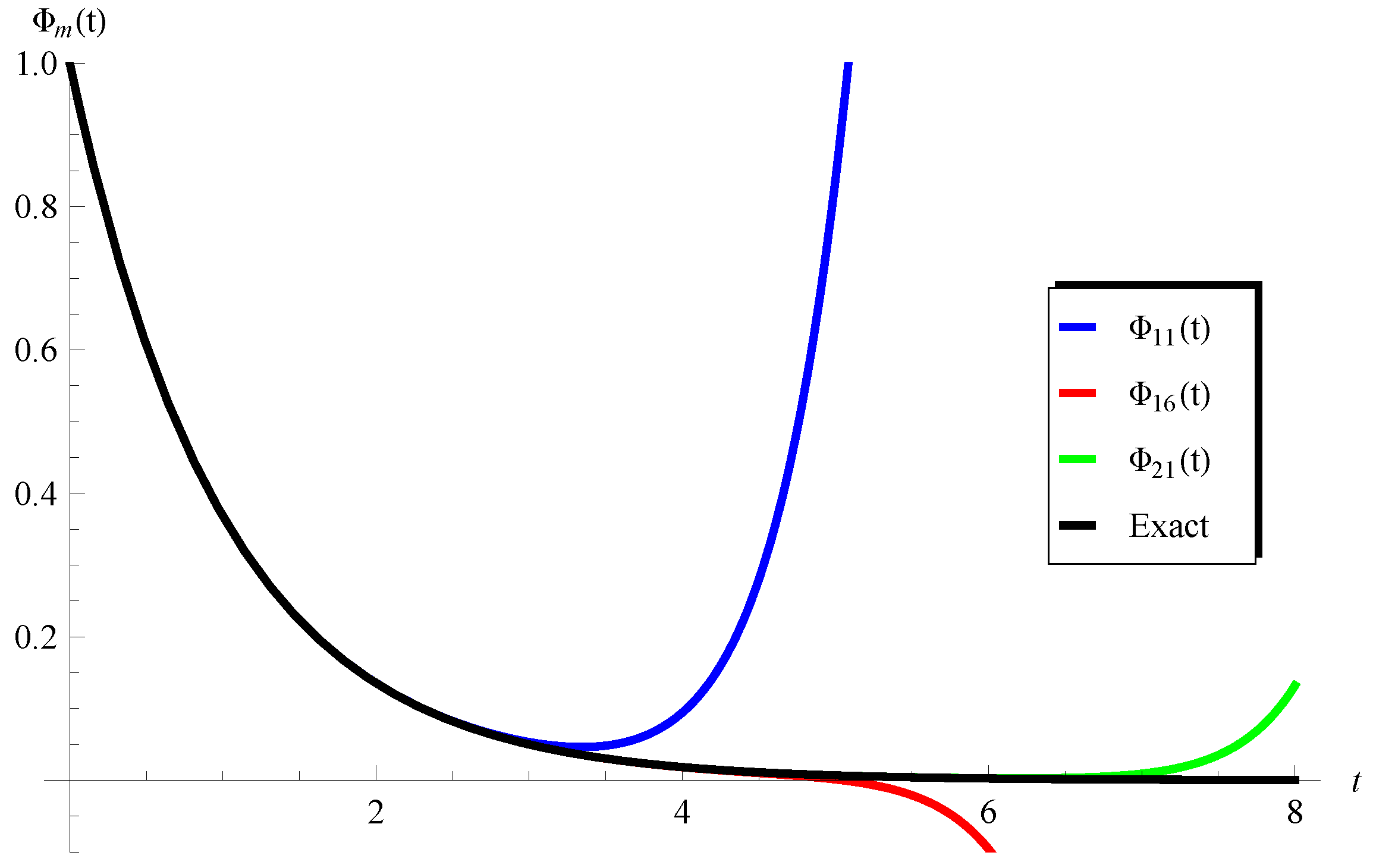
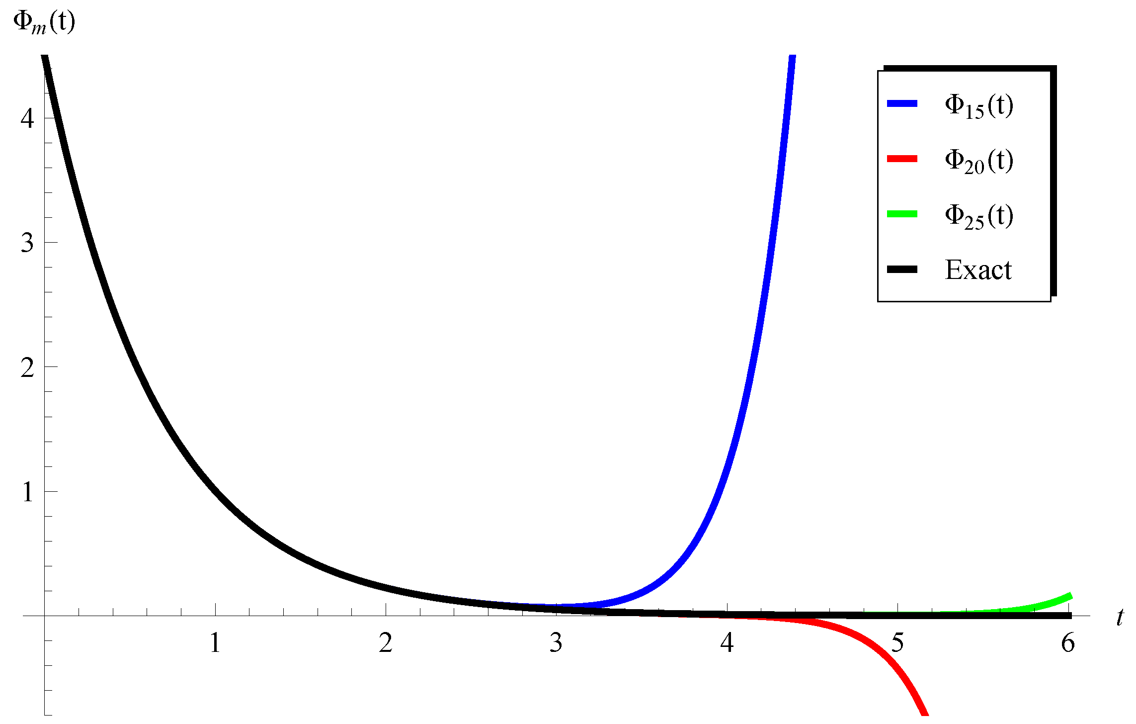
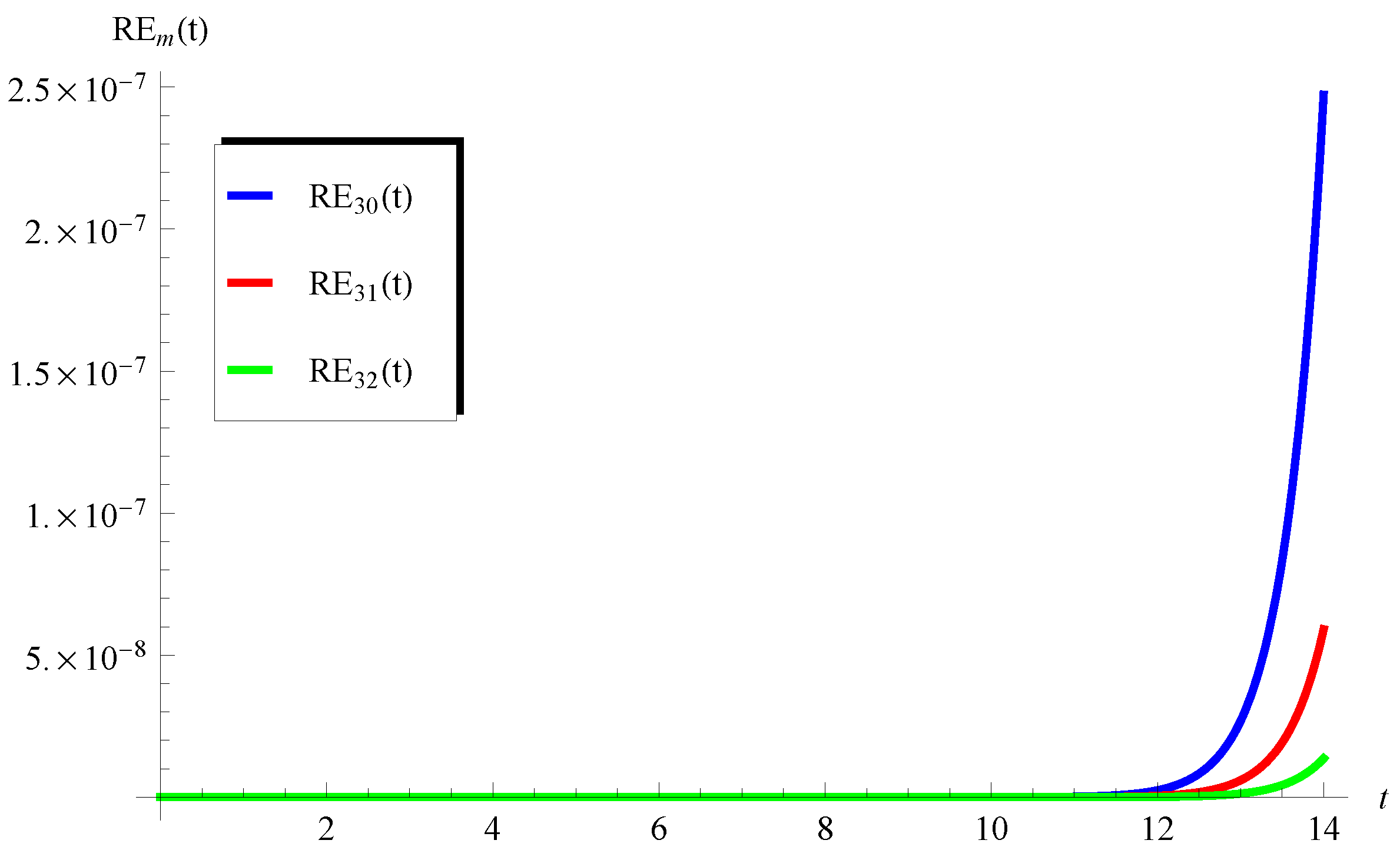
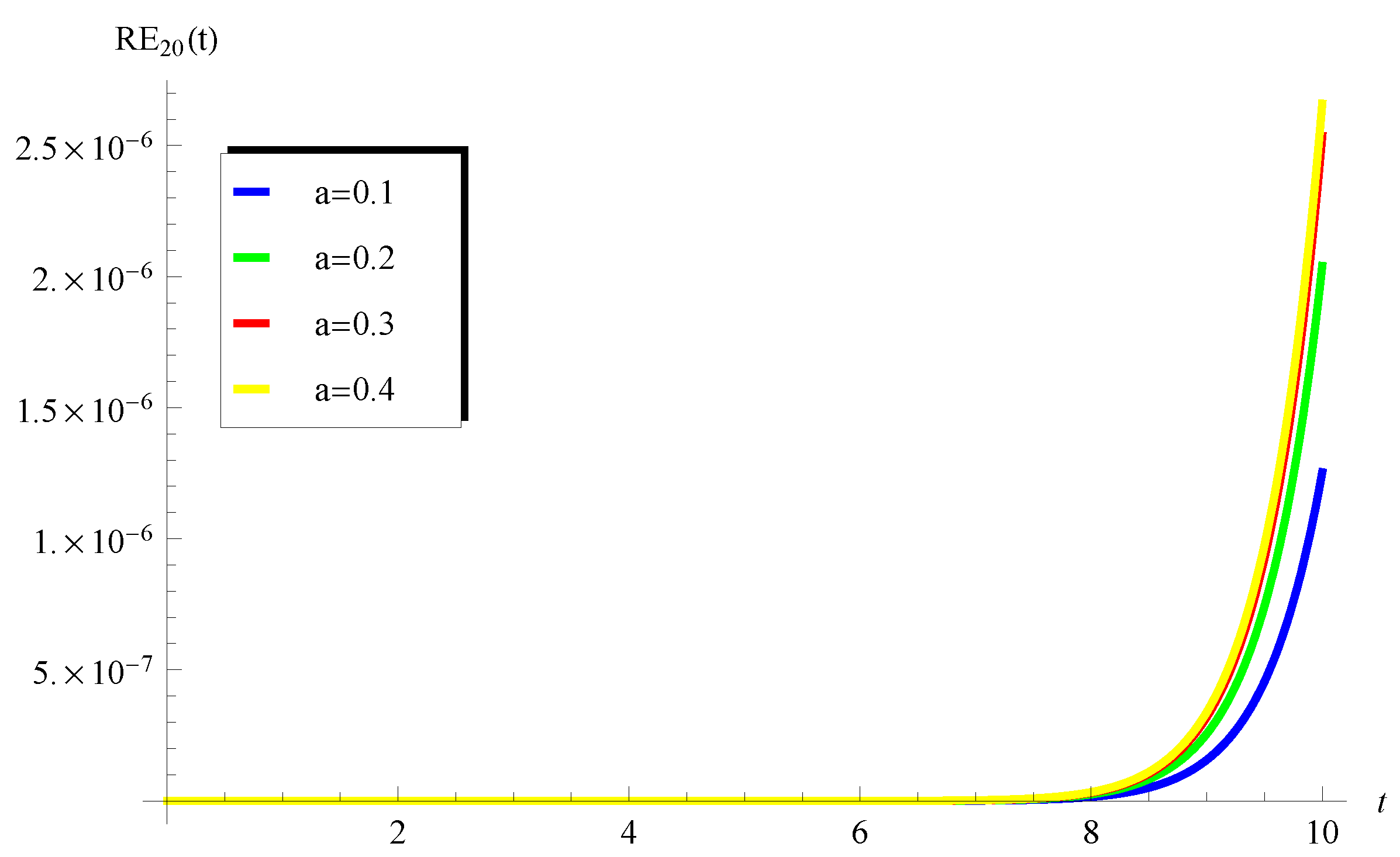
5.2. Validation of Accuracy

This part is devoted to examining the validity of the closed form series solution (14) to give accurate approximations. The m-term approximate solution ${\mathsf{\Phi }}_m\left(t\right)$ can be extracted from (14) by replacing infinity by a finite number of terms, thus,

$${\mathsf{\Phi }}_m\left(t\right)=\lambda +\frac{\alpha }{\beta }\left(e^{\beta t}-1\right)+\sum _{n=1}^m\frac{t^n}{n!}\left(\lambda +\sum _{j=0}^{n-2}\frac{\alpha {\beta }^j}{{\prod }_{k=0}^{j}h\left(k\right)}\right)\prod _{k=0}^{n-1}h\left(k\right),m\ge 2.$$

(42)

Figure 1 shows the comparison between the approximations ${\mathsf{\Phi }}_m\left(t\right)$, $m=11,16,21$ and the exact solution $y\left(t\right)=e^{-t}$ for the model (32) at $c=\frac{3}{4}$. It is clear from this figure that the approximations ${\mathsf{\Phi }}_m\left(t\right)$ approaches the exact solution and the domain of agreement is enlarged by increasing the number of terms m. In addition, Figure 2 and Figure 3 confirm this conclusion at different values of the involved parameters.

The accuracy of the approximations ${\mathsf{\Phi }}_m\left(t\right)$ can be examined/validated by calculating the residual error $R{E}_m\left(t\right)$ defined by

$$R{E}_m\left(t\right)=\left|{\mathsf{\Phi }}_m^{\prime }\left(t\right)-a{\mathsf{\Phi }}_m\left(t\right)-b{\mathsf{\Phi }}_m\left(ct\right)-\alpha e^{\beta t}\right|,m\ge 2.$$

(43)

In Figure 4 and Figure 5, the residual errors $R{E}_m\left(t\right)$, $m=30,31,32$ are displayed at $\lambda =1$, $a=-\frac{1}{2}$, $b=\frac{1}{3}$, $\alpha =\frac{1}{4}$, $\beta =-\frac{1}{2}$ when $c=\frac{1}{5}$ (Figure 4) and $c=\frac{9}{10}$ (Figure 5). The numerical results show acceptable accuracy, especially when the number of terms increases. Furthermore, the influence of the parameter a on the residual error $R{E}_{20}\left(t\right)$ is depicted in Figure 6 at $\lambda =1$, $b=\frac{1}{3}$, $c=-\frac{1}{2}$, $\alpha =\frac{1}{4}$, and $\beta =-\frac{1}{20}$. This figure indicates that the residual $R{E}_{20}\left(t\right)$ increases by the increase in a while Figure 7 declares a converse behaviour for the influence of the parameter b on the residual error $R{E}_{20}\left(t\right)$. The above discussion reveals the effectiveness and efficiency of the proposed analysis which can be implemented to analyze other forms of the inhomogeneous pantograph equation.

6. Conclusions

The inhomogeneous version of the pantograph equation was investigated in this paper. The exponential function was incorporated as an inhomogeneous term of the pantograph equation. The MSE is applied in a straightforward manner to solve the present model of the inhomogeneous pantograph equation. The solution was successfully obtained in a closed series form, where a general/unified formula was given for the series coefficients. The convergence issue was addressed and proved theoretically. The results obtained in this article generalize previously obtained/known results in the relevant literature. The accuracy of the current calculations are verified via performing several comparisons with the available exact solutions of some mathematical models in the relevant literature. The calculated residuals showed that the the present approximations enjoyed acceptable accuracy.

The effectiveness and efficiency of the proposed approach deserves further extension to include other complex models including different types of inhomogeneous terms and also other ways of describing delay, namely the memory effect. The current approach can also be used to describe delayed processes within mathematical models using fractional derivatives [28].

References

1. Sezera, M.; Akyüz-Dascıoglub, A. A Taylor method for numerical solution of generalized pantograph equations with linear functional argument. J. Comput. Appl. Math. 2007, 200, 217–225. [Google Scholar] [CrossRef]
2. Sedaghat, S.; Ordokhani, Y.; Dehghan, M. Numerical solution of the delay differential equations of pantograph type via Chebyshev polynomials. Commun. Nonlinear Sci. Numer. Simul. 2012, 17, 4815–4830. [Google Scholar] [CrossRef]
3. Tohidi, E.; Bhrawy, A.H.; Erfani, K. A collocation method based on Bernoulli operational matrix for numerical solution of generalized pantograph equation. Appl. Math. Model. 2013, 37, 4283–4294. [Google Scholar] [CrossRef]
4. Javadi, S.; Babolian, E.; Taheri, Z. Solving generalized pantograph equations by shifted orthonormal Bernstein polynomials. J. Comput. Appl. Math. 2016, 303, 1–4. [Google Scholar] [CrossRef]
5. Shen, J.; Tang, T.; Wang, L. Spectral Methods: Algorithms, Analysis and Applications; Springer: Berlin/Heidelberg, Germany, 2011; Volume 41. [Google Scholar]
6. Jafari, H.; Mahmoudi, M.; Noori Skandari, M.H. A new numerical method to solve pantograph delay differential equations with convergence analysis. Adv. Differ. Equ. 2021, 2021, 129. [Google Scholar] [CrossRef]
7. Ezz-Eldien, S.S. On solving systems of multi-pantograph equations via spectral tau method. Appl. Math. Comput. 2018, 321, 63–73. [Google Scholar] [CrossRef]
8. Isik, O.R.; Turkoglu, T. A rational approximate solution for generalized pantograph-delay differential equations. Math. Methods Appl. Sci. 2016, 39, 2011–2024. [Google Scholar] [CrossRef]
9. Andrews, H.I. Third paper: Calculating the behaviour of an overhead catenary system for railway electrification. Proc. Inst. Mech. Eng. 1964, 179, 809–846. [Google Scholar] [CrossRef]
10. Gilbert, G.; Davtcs, H.E.H. Pantograph motion on a nearly uniform railway overhead line. Proc. Inst. Electr. Eng. 1966, 113, 485–492. [Google Scholar] [CrossRef]
11. Caine, P.M.; Scott, P.R. Single-wire railway overhead system. Proc. Inst. Electr. Eng. 1969, 116, 1217–1221. [Google Scholar] [CrossRef]
12. Abbott, M.R. Numerical method for calculating the dynamic behaviour of a trolley wire overhead contact system for electric railways. Comput. J. 1970, 13, 363–368. [Google Scholar] [CrossRef]
13. Ockendon, J.; Tayler, A.B. The dynamics of a current collection system for an electric locomotive. Proc. R. Soc. Lond. A Math. Phys. Eng. Sci. 1971, 322, 447–468. [Google Scholar]
14. Al-Enazy, A.H.S.; Ebaid, A.; Algehyne, E.A.; Al-Jeaid, H.K. Advanced Study on the Delay Differential Equation y(t) = ay(t) + by(ct). Mathematics 2022, 10, 4302. [Google Scholar] [CrossRef]
15. Albidah, A.B.; Kanaan, N.E.; Ebaid, A.; Al-Jeaid, H.K. Exact and Numerical Analysis of the Pantograph Delay Differential Equation via the Homotopy Perturbation Method. Mathematics 2023, 11, 944. [Google Scholar] [CrossRef]
16. El-Zahar, E.R.; Ebaid, A. Analytical and Numerical Simulations of a Delay Model: The Pantograph Delay Equation. Axioms 2022, 11, 741. [Google Scholar] [CrossRef]
17. Alrebdi, R.; Al-Jeaid, H.K. Accurate Solution for the Pantograph Delay Differential Equation via Laplace Transform. Mathematics 2023, 11, 2031. [Google Scholar] [CrossRef]
18. Khaled, S.M. Applications of Standard Methods for Solving the Electric Train Mathematical Model with Proportional Delay. Int. J. Anal. Appl. 2022, 20, 27. [Google Scholar] [CrossRef]
19. Ebaid, A.; Al-Jeaid, H.K. On the Exact Solution of the Functional Differential Equation y(t) = ay(t) + by(−t). Adv. Differ. Equ. Control Processes 2022, 26, 39–49. [Google Scholar] [CrossRef]
20. Bakodah, H.O.; Ebaid, A. Exact solution of Ambartsumian delay differential equation and comparison with Daftardar-Gejji and Jafari approximate method. Mathematics 2018, 6, 331. [Google Scholar] [CrossRef]
21. Ebaid, A.; Cattani, C.; Al Juhani, A.S.; El-Zahar, E.R. A novel exact solution for the fractional Ambartsumian equation. Adv. Differ. Equ. 2021, 2021, 88. [Google Scholar] [CrossRef]
22. Dogan, N. Solution of the system of ordinary differential equations by combined Laplace transform-Adomian decomposition method. Math. Comput. Appl. 2012, 17, 203–211. [Google Scholar] [CrossRef]
23. Atangana, A.; Alkaltani, B.S. A novel double integral transform and its applications. J. Nonlinear Sci. Appl. 2016, 9, 424–434. [Google Scholar] [CrossRef]
24. Khaled, S.M. The exact effects of radiation and joule heating on Magnetohydrodynamic Marangoni convection over a flat surface. Therm. Sci. 2018, 22, 63–72. [Google Scholar] [CrossRef]
25. Venkata Pavani, P.; Lakshmi Priya, U.; Amarnath Reddy, B. Solving differential equations by using Laplace transforms. Int. J. Res. Anal. Rev. 2018, 5, 1796–1799. [Google Scholar]
26. Alrebdi, R.; Al-Jeaid, H.K. Two Different Analytical Approaches for Solving the Pantograph Delay Equation with Variable Coefficient of Exponential Order. Axioms 2024, 13, 229. [Google Scholar] [CrossRef]
27. Kac, V.G.; Cheung, P. Quantum Calculus; Springer: New York, NY, USA, 2002. [Google Scholar]
28. Petras, I. Fractional-Order Nonlinear Systems: Modeling, Analysis and Simulation; Beijing and Springer-Verlag; Springer: Berlin/Heidelberg, Germany, 2011; ISBN 9783642181009. [Google Scholar]
Figure 1. Comparison between the approximations Φ m ( t ) , m = 11 , 16 , 21 and the exact solution y ( t ) = e t for the model (33) at c = 3 4 .
Axioms 13 00377 g001
Figure 2. Comparison between the approximations Φ m ( t ) , m = 15 , 20 , 25 and the exact solution y ( t ) = 9 2 e 3 t 2 for the model (39) at a = 3 2 , b = 2 , α = 9 , and c = 1 2 .
Axioms 13 00377 g002
Figure 3. Comparison between the approximations Φ m ( t ) , m = 10 , 13 , 16 and the exact solution y ( t ) = e t for the model (39) at a = 1 , b = 1 2 , α = 1 2 , and c = 1 3 .
Axioms 13 00377 g003
Figure 4. The residual errors R E m ( t ) , m = 30 , 31 , 32 at λ = 1 , a = 1 2 , b = 1 3 , α = 1 4 , β = 1 2 , and c = 1 5 .
Axioms 13 00377 g004
Figure 5. The residual errors R E m ( t ) , m = 30 , 31 , 32 at λ = 1 , a = 1 2 , b = 1 3 , α = 1 4 , β = 1 2 , and c = 9 10 .
Axioms 13 00377 g005
Figure 6. Influence of the parameter a on the residual errors R E 20 ( t ) at λ = 1 , b = 1 3 , c = 1 2 , α = 1 4 , and β = 1 20 .
Axioms 13 00377 g006
Figure 7. Influence of the parameter b on the residual errors R E 20 ( t ) at λ = 0 , a = 1 , c = 1 2 , α = 1 4 , and β = 1 2 .
Axioms 13 00377 g007
Disclaimer/Publisher’s Note: The statements, opinions and data contained in all publications are solely those of the individual author(s) and contributor(s) and not of MDPI and/or the editor(s). MDPI and/or the editor(s) disclaim responsibility for any injury to people or property resulting from any ideas, methods, instructions or products referred to in the content.