

Analysis of Fat Big Data Using Factor Models and Penalization Techniques: A Monte Carlo Simulation and Application


Abstract
1. Introduction
- Fat·Big·Data: the length of covariates (large P) exceeds the number of observations (large N);
- Tall·Big·Data: the length of covariates (large P) is considerably lower than the number of observations (sufficient large N);
- Huge·Big·Data: the length of covariates (large P) is lower than the number of observations (large N).
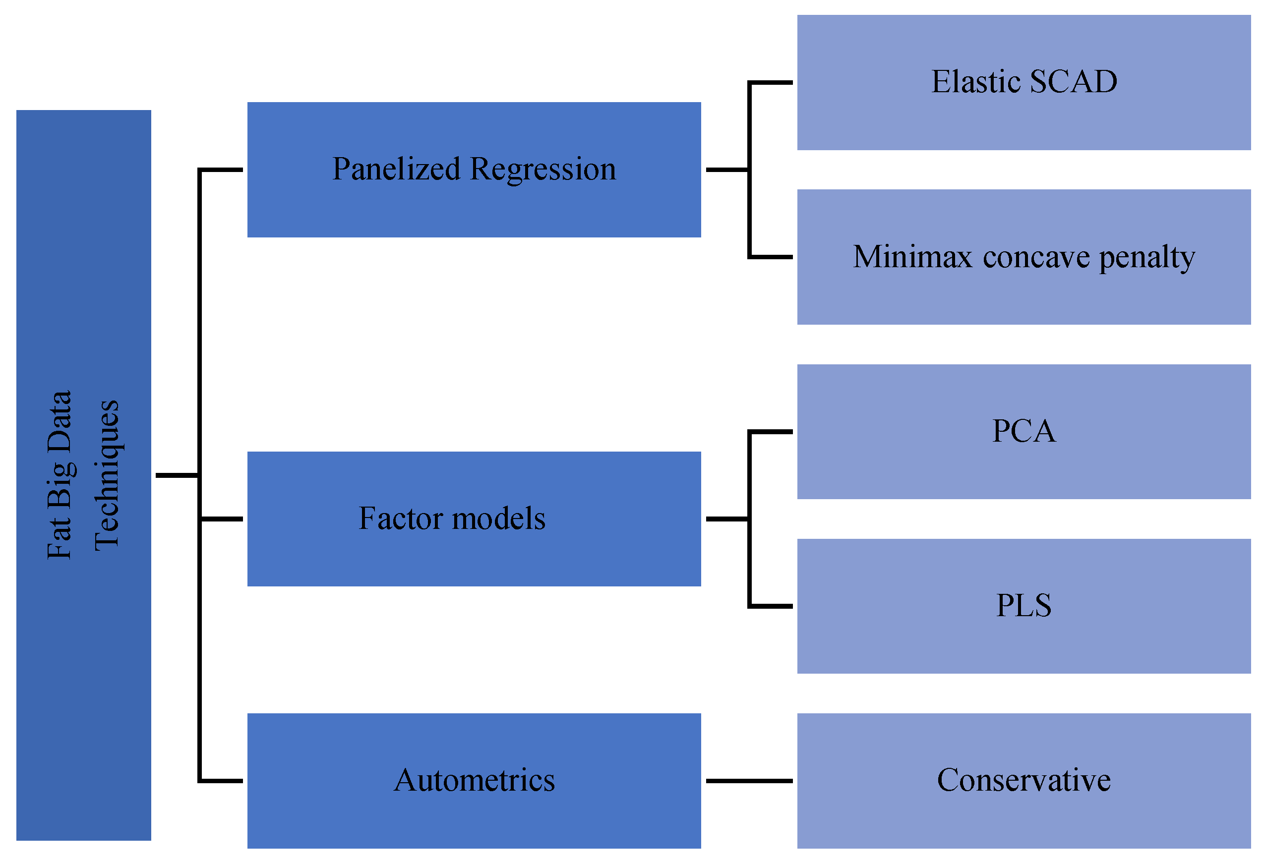
2. Methods
2.1. Factor Models
2.2. Panelized Regression and Classical Approach
Panelized·Regression·Methods
2.3. Classical Approach
3. Monte Carlo Evidence on Forecasting Performance
3.1. Data·Generating·Process (DGP)
3.2. Simulation Results
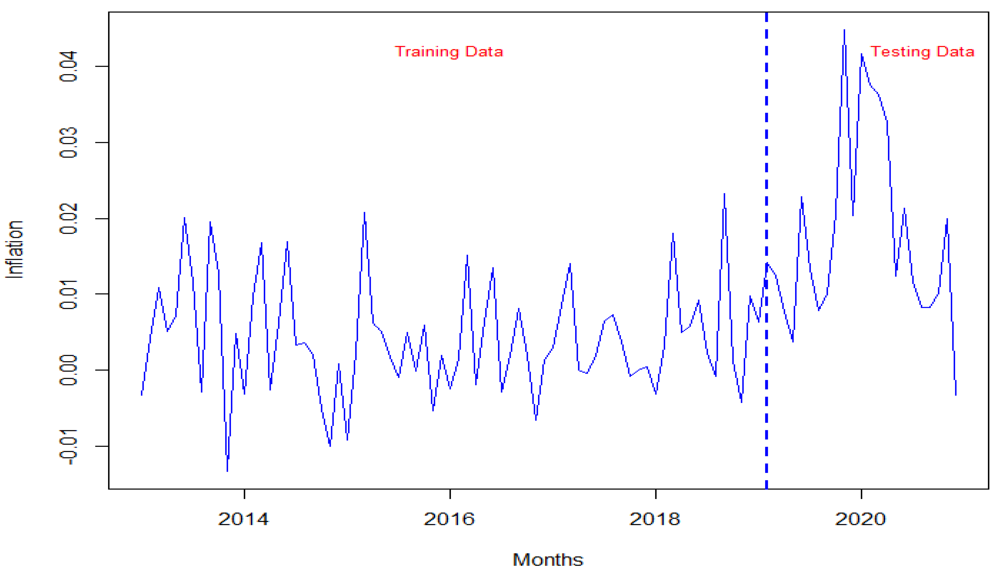
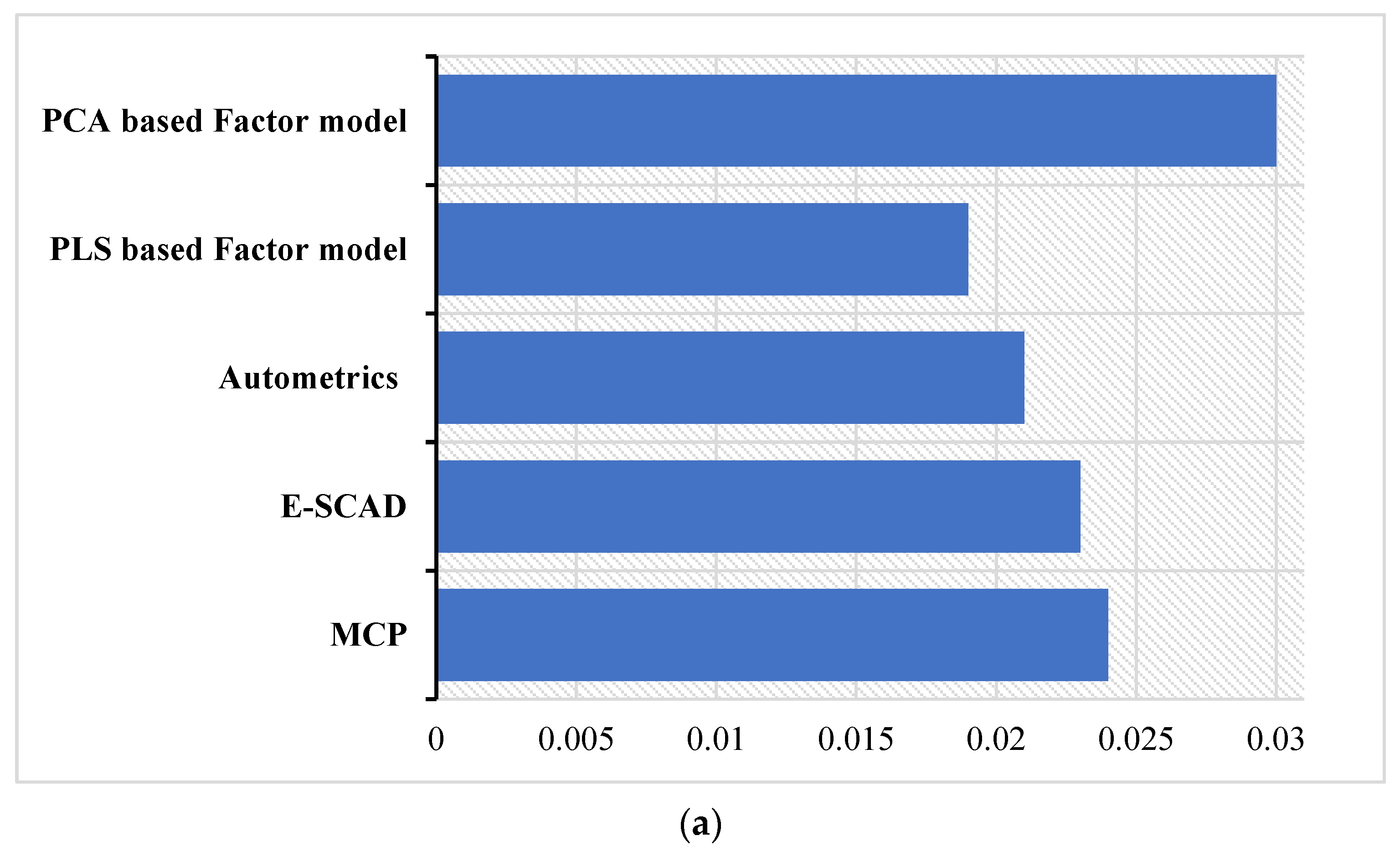
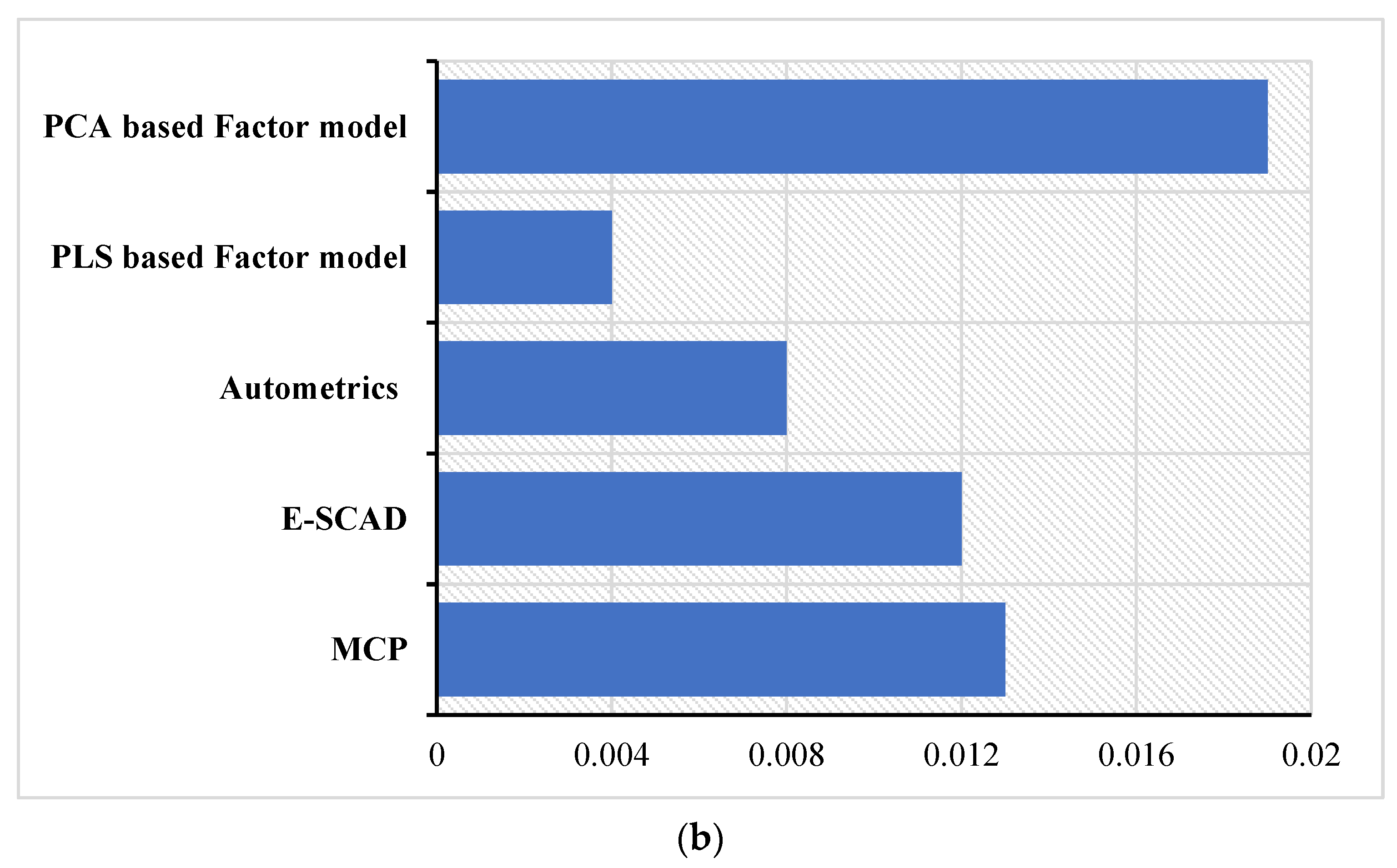
4. Testing on Empirical Dataset
Out-of-Sample Inflation Forecasting
5. Discussion, Implications, and Limitations
5.1. Discussion
5.2. Implication
5.3. Limitations and Future Avenue
Author Contributions
Funding
Data Availability Statement
Conflicts of Interest
Appendix A

| Sr. no | Name of the Variables |
|---|---|
| Real Sector (Output) | |
| 1 | Production of Sugar (SA) |
| 2 | Production of Vegetable (SA) |
| 3 | Production of Cigarettes (SA) |
| 4 | Production of Cotton yarn (SA) |
| 5 | Production of Cotton Cloth (SA) |
| 6 | Production of Paper (SA) |
| 7 | Production of Paper Board (SA) |
| 8 | Production of Soda Ash (SA) |
| 9 | Production of Caustic Soda (SA) |
| 10 | Production of Sulfuric Acid (SA) |
| 11 | Production of Chlorine Gas (SA) |
| 12 | Production of Urea (SA) |
| 13 | Production of Super Phosphate (SA) |
| 14 | Production of Ammonium Nitrate (SA) |
| 15 | Production of Nitro Phosphate (SA) |
| 16 | Production of Cycle Tyres and Tubes (SA) |
| 17 | Production of Motor Tyres and Tubes (SA) |
| 18 | Production of Cement (SA) |
| 19 | Production of Tractors (SA) |
| 20 | Production of Bicycle (SA) |
| 21 | Production of Silica Sand (SA) |
| 22 | Production of Gypsum (SA) |
| 23 | Production of Limestone (SA) |
| 24 | Production of Rock Salt (SA) |
| 25 | Production of Coal (SA) |
| 26 | Production of Chromate (SA) |
| 27 | Production of Crude Oil (SA) |
| 28 | Production of Natural Gas (SA) |
| 29 | Production of Electricity (SA) |
| Monetary Sector (Money, Reserves and Banking System) Money | |
| 30 | Currency in circulation |
| 31 | Bank Deposit with State Bank of Pakistan |
| 32 | Other Deposit with State Bank of Pakistan |
| 33 | Currency in Tills of Scheduled Banks |
| 34 | Demand Deposits |
| 35 | Time Deposits |
| 36 | Resident Foreign Currency Deposits |
| 37 | Government Sector Borrowing (net) |
| 38 | Budgetary Support |
| 39 | Commodity Operations |
| 40 | Credit to Private Sector |
| 41 | Credit to Public Sector Enterprises |
| 42 | Net Foreign (Domestic) Assets of State Bank of Pakistan |
| 43 | Net Foreign Assets of the Scheduled Banks in Pakistan |
| Prices | |
| 44 | Consumer Price Index |
| 45 | Consumer Price Index (Food) |
| 46 | Wholesale Price Index |
| 47 | Sensitive Price Index |
| Exchange Rates | |
| 48 | Nominal Effective Exchange Rate |
| 49 | Real Effective Exchange Rate |
| 50 | Saudi Arabian Riyal (Monthly Average) |
| 51 | UAE Dirham (Monthly Average) |
| 52 | US Dollar (Monthly Average) |
| 53 | Canadian Dollar (Monthly Average) |
| 54 | UK Pound Sterling (Monthly Average) |
| 55 | Euro (Monthly Average) |
| 56 | Japanese Yen (Monthly Average) |
| Interest Rates | |
| 57 | Lending Weighted Average Rates |
| 58 | Deposits Weighted Average Rates |
| 59 | Call Money Rate |
| 60 | Overnight Weighted Average Repo Rate (all data) |
| 61 | Karachi Interbank Offered Rate 1 Week |
| 62 | Karachi Interbank Offered Rate 2 Weeks |
| 63 | Karachi Interbank Offered Rate 1 Month |
| 64 | Karachi Interbank Offered Rate 3 Months |
| 65 | Karachi Interbank Offered Rate 6 Months |
| 66 | Karachi Interbank Offered Rate 9 Months |
| 67 | Karachi Interbank Offered Rate 12 Months |
| External Sector | |
| 68 | Exports |
| 69 | Imports |
| 70 | Workers Remittances |
| 71 | Gold Reserves |
| 72 | Foreign Exchange Reserves with State Bank of Pakistan |
| 73 | Foreign Exchange Reserves with Scheduled Banks in Pakistan |
| 74 | Old Foreign Currency Accounts |
| 75 | New Foreign Currency Accounts (FE-25) |
| Fiscal Sector | |
| 76 | Federal Government Direct Tax Collection |
| 77 | Federal Government Indirect Tax (Sales Tax) |
| 78 | Federal Government Indirect Tax (Excise Tax) |
| 79 | Federal Government Indirect Tax (Customs) |
References
- Filzmoser, P.; Nordhausen, K. Robust linear regression for high-dimensional data: An overview. Wiley Interdiscip. Rev. Comput. Stat. 2021, 13, e1524. [Google Scholar] [CrossRef]
- Gujarati, D.N.; Porter, D.C.; Gunasekar, S. Basic Econometrics; Tata McGraw-Hill Education: New York, NY, USA, 2012. [Google Scholar]
- Kim, H.H.; Swanson, N.R. Mining Big Data Using Parsimonious Factor and Shrinkage Methods; Working paper; Rutgers University: New Brunswick, NJ, USA, 2013. [Google Scholar]
- Stock, J.H.; Watson, M.W. Macroeconomic forecasting using diffusion indexes. J. Bus. Econ. Stat. 2002, 20, 147–162. [Google Scholar] [CrossRef]
- Stock, J.H.; Watson, M.W. Generalized shrinkage methods for forecasting using many predictors. J. Bus. Econ. Stat. 2012, 30, 481–493. [Google Scholar] [CrossRef]
- Hansen, C.; Liao, Y. The factor-lasso and k-step bootstrap approach for inference in high-dimensional economic applications. Econom. Theory 2019, 35, 465–509. [Google Scholar] [CrossRef]
- Bai, J.; Liao, Y. Efficient estimation of approximate factor models via penalized maximum likelihood. J. Econom. 2016, 191, 1–18. [Google Scholar] [CrossRef]
- Fan, J.; Ke, Y.; Liao, Y. Robust factor models with explanatory proxies. arXiv 2016, arXiv:1603.07041. [Google Scholar] [CrossRef]
- Fan, J.; Liao, Y.; Wang, W. Projected principal component analysis in factor models. Ann. Stat. 2016, 44, 219. [Google Scholar] [CrossRef]
- Fan, J.; Xue, L.; Yao, J. Sufficient forecasting using factor models. J. Econom. 2017, 201, 292–306. [Google Scholar] [CrossRef]
- Bernanke, B.S.; Boivin, J.; Eliasz, P. Measuring the effects of monetary policy: A factor-augmented vector autoregressive (FAVAR) approach. Q. J. Econ. 2005, 120, 387–422. [Google Scholar]
- Syed, A.A.S.; Lee, K.H. Macroeconomic forecasting for Pakistan in a data-rich environment. Appl. Econ. 2021, 53, 1077–1091. [Google Scholar] [CrossRef]
- Tibshirani, R. Regression shrinkage and selection via the lasso. J. R. Stat. Soc. Ser. B (Methodol.) 1996, 58, 267–288. [Google Scholar] [CrossRef]
- Fan, J.; Li, R. Variable Selection via Nonconcave Penalized Likelihood and its Oracle Properties. J. Am. Stat. Assoc. 2001, 96, 1348–1360. [Google Scholar] [CrossRef]
- Zou, H.; Hastie, T. Regularization and variable selection via the elastic net. J. R. Stat. Soc. Ser. B (Stat. Methodol.) 2005, 67, 301–320. [Google Scholar] [CrossRef]
- Zou, H. The adaptive lasso and its oracle properties. J. Am. Stat. Assoc. 2006, 101, 1418–1429. [Google Scholar] [CrossRef]
- Zou, H.; Zhang, H.H. On the adaptive elastic-net with a diverging number of parameters. Ann. Stat. 2009, 37, 1733. [Google Scholar] [CrossRef] [PubMed]
- Zhang, C.H. Nearly unbiased variable selection under minimax concave penalty. Ann. Stat. 2010, 38, 894–942. [Google Scholar] [CrossRef] [PubMed]
- Zeng, L.; Xie, J. Group variable selection via SCAD-L 2. Statistics 2014, 48, 49–66. [Google Scholar] [CrossRef]
- Bai, J.; Ng, S. Forecasting economic time series using targeted predictors. J. Econom. 2008, 146, 304–317. [Google Scholar] [CrossRef]
- De Mol, C.; Giannone, D.; Reichlin, L. Forecasting using a large number of predictors: Is Bayesian shrinkage a valid alternative to principal components? J. Econom. 2008, 146, 318–328. [Google Scholar] [CrossRef]
- Castle, J.L.; Clements, M.P.; Hendry, D.F. Forecasting by factors, by variables, by both or neither? J. Econom. 2013, 177, 305–319. [Google Scholar] [CrossRef]
- Luciani, M. Forecasting with approximate dynamic factor models: The role of non-pervasive shocks. Int. J. Forecast. 2014, 30, 20–29. [Google Scholar] [CrossRef]
- Doornik, J.A.; Hendry, D.F. Statistical model selection with big data. Cogent Econ. Financ. 2015, 3, 1045216. [Google Scholar] [CrossRef]
- Kristensen, J.T. Diffusion indexes with sparse loadings. J. Bus. Econ. Stat. 2017, 35, 434–451. [Google Scholar] [CrossRef]
- Li, J.; Chen, W. Forecasting macroeconomic time series: LASSO-based approaches and their forecast combinations with dynamic factor models. Int. J. Forecast. 2014, 30, 996–1015. [Google Scholar] [CrossRef]
- Marsilli, C. Variable Selection in Predictive MIDAS Models. Banque de France Working Paper No. 520. 2014. Available online: https://papers.ssrn.com/sol3/papers.cfm?abstract_id=2531339 (accessed on 17 June 2024).
- Nicholson, W.; Matteson, D.; Bien, J. BigVAR: Tools for modeling sparse high-dimensional multivariate time series. arXiv 2017, arXiv:1702.07094. [Google Scholar]
- Kim, H.H.; Swanson, N.R. Forecasting financial and macroeconomic variables using data reduction methods: New empirical evidence. J. Econom. 2014, 178, 352–367. [Google Scholar] [CrossRef]
- Kim, H.H.; Swanson, N.R. Mining big data using parsimonious factor, machine learning, variable selection and shrinkage methods. Int. J. Forecast. 2018, 34, 339–354. [Google Scholar] [CrossRef]
- Swanson, N.R.; Xiong, W. Big data analytics in economics: What have we learned so far, and where should we go from here? Can. J. Econ. 2018, 51, 695–746. [Google Scholar] [CrossRef]
- Swanson, N.R.; Xiong, W.; Yang, X. Predicting interest rates using shrinkage methods, real-time diffusion indexes, and model combinations. J. Appl. Econom. 2020, 35, 587–613. [Google Scholar] [CrossRef]
- Smeekes, S.; Wijler, E. Macroeconomic forecasting using penalized regression methods. Int. J. Forecast. 2018, 34, 408–430. [Google Scholar] [CrossRef]
- Tu, Y.; Lee, T.H. Forecasting using supervised factor models. J. Manag. Sci. Eng. 2019, 4, 12–27. [Google Scholar] [CrossRef]
- Kim, H.; Ko, K. Improving forecast accuracy of financial vulnerability: PLS factor model approach. Econ. Model. 2020, 88, 341–355. [Google Scholar] [CrossRef]
- Maehashi, K.; Shintani, M. Macroeconomic forecasting using factor models and machine learning: An application to Japan. J. Jpn. Int. Econ. 2020, 58, 101104. [Google Scholar] [CrossRef]
- Abdić, A.; Resić, E.; Abdić, A. Modelling and forecasting GDP using factor model: An empirical study from Bosnia and Herzegovina. Croat. Rev. Econ. Bus. Soc. Stat. 2020, 6, 10–26. [Google Scholar] [CrossRef]
- Kim, H.; Shi, W.; Kim, H.H. Forecasting financial stress indices in Korea: A factor model approach. Empir. Econ. 2020, 59, 2859–2898. [Google Scholar] [CrossRef]
- Kim, H.; Shi, W. Forecasting financial vulnerability in the USA: A factor model approach. J. Forecast. 2021, 40, 439–457. [Google Scholar] [CrossRef]
- Khan, F.; Urooj, A.; Khan, S.A.; Alsubie, A.; Almaspoor, Z.; Muhammadullah, S. Comparing the Forecast Performance of Advanced Statistical and Machine Learning Techniques Using Huge Big Data: Evidence from Monte Carlo Experiments. Complexity 2021, 2021, 6117513. [Google Scholar] [CrossRef]
- Kelly, B.T.; Kuznetsov, B.; Malamud, S.; Xu, T.A. Deep Learning from Implied Volatility Surfaces; Swiss Finance Institute Research Paper; Swiss Finance Institute: Zürich, Switzerland, 2023; pp. 23–60. [Google Scholar]
- Kelly, B.; Kuznetsov, B.; Malamud, S.; Xu, T.A. Large (and Deep) Factor Models. arXiv 2024, arXiv:2402.06635. [Google Scholar] [CrossRef]
- Kozak, S.; Nagel, S. When Do Cross-Sectional Asset Pricing Factors Span the Stochastic Discount Factor? (No. w31275); National Bureau of Economic Research: Cambridge, MA, USA, 2023. [Google Scholar]
- Didisheim, A.; Ke, S.B.; Kelly, B.T.; Malamud, S. Complexity in Factor Pricing Models (No. w31689); National Bureau of Economic Research: Cambridge, MA, USA, 2023. [Google Scholar]
- Chen, L.; Pelger, M.; Zhu, J. Deep learning in asset pricing. Manag. Sci. 2024, 70, 714–750. [Google Scholar] [CrossRef]
- Fan, J.; Ke, Z.T.; Liao, Y.; Neuhierl, A. Structural Deep Learning in Conditional Asset Pricing. Available at SSRN 4117882. 2022. Available online: https://static1.squarespace.com/static/5d6417169b0edd0001903770/t/655524542cbf566e3801a2ed/1700078678513/guilherme+piancetino.pdf (accessed on 17 June 2024).
- Stock, J.H.; Watson, M.W. Forecasting inflation. J. Monet. Econ. 1999, 44, 293–335. [Google Scholar] [CrossRef]
- Castle, J.L.; Doornik, J.A.; Hendry, D.F. Modelling non-stationary ‘Big Data’. Int. J. Forecast. 2021, 37, 1556–1575. [Google Scholar] [CrossRef]
- Khan, F.; Urooj, A.; Khan, S.A.; Khosa, S.K.; Muhammadullah, S.; Almaspoor, Z. Evaluating the performance of feature selection methods using huge big data: A Monte Carlo simulation approach. Math. Probl. Eng. 2022, 2022, 6607330. [Google Scholar] [CrossRef]
- Stock, J.H.; Watson, M.W. Forecasting using principal components from a large number of predictors. J. Am. Stat. Assoc. 2002, 97, 1167–1179. [Google Scholar] [CrossRef]
- Bai, J.; Ng, S. Confidence intervals for diffusion index forecasts and inference for factor-augmented regressions. Econometrica 2006, 74, 1133–1150. [Google Scholar] [CrossRef]
- Bai, J.; Ng, S. Determining the number of factors in approximate factor models. Econometrica 2002, 70, 191–221. [Google Scholar] [CrossRef]
- Bai, J.; Ng, S. Evaluating latent and observed factors in macroeconomics and finance. J. Econom. 2006, 131, 507–537. [Google Scholar] [CrossRef]
- Boivin, J.; Ng, S. Are more data always better for factor analysis? J. Econom. 2006, 132, 169–194. [Google Scholar] [CrossRef]
- Wold, H. Soft Modelling: The Basic Design and Some Extensions, Vol. 1 of Systems under Indirect Observation, Part II; North-Holland: Amsterdam, The Netherlands, 1982. [Google Scholar]
- Pascual Herrero, H. Least Squares Regression Principal Component Analysis. Bachelor’s Thesis, Universitat Politècnica de Catalunya, Barcelona, Spain, 2020. [Google Scholar]
- Wang, Y.; Fan, Q.; Zhu, L. Variable selection and estimation using a continuous approximation to the L0 penalty. Ann. Inst. Stat. Math. 2018, 70, 191–214. [Google Scholar] [CrossRef]
- Li, N.; Yang, H. Nonnegative estimation and variable selection under minimax concave penalty for sparse high-dimensional linear regression models. Stat. Pap. 2021, 62, 661–680. [Google Scholar] [CrossRef]
- Khan, F.; Urooj, A.; Ullah, K.; Alnssyan, B.; Almaspoor, Z. A Comparison of Autometrics and Penalization Techniques under Various Error Distributions: Evidence from Monte Carlo Simulation. Complexity 2021, 2021, 9223763. [Google Scholar] [CrossRef]


| Models | ∑ = 0.25, P = 130 | ∑ = 0.25, P = 150 | ||
|---|---|---|---|---|
| n = 50/100/125 | RMSE | MAE | RMSE | MAE |
| MCP | 6.86/5.41/2.243 | 5.602/4.375/1.811 | 6.043/3.319/1.208 | 4.970/2.681/0.975 |
| E-SCAD | 5.80/2.00/1.355 | 4.741/1.620/1.095 | 4.899/1.364/1.257 | 4.008/1.098/1.016 |
| Autometrics | 4.192/1.312/1.189 | 3.419/1.058/0.957 | 3.267/1.222/1.145 | 2.673/0.986/0.924 |
| PLS_FM | 4.530/3.213/2.727 | 3.678/2.589/2.197 | 5.260/3.786/3.295 | 4.309/3.062/2.623 |
| PCA_FM | 6.475/5.781/5.695 | 5.725/4.685/4.589 | 6.512/6.398/6.342 | 5.318/5.166/5.104 |
| n = 50/100/125 | ∑ = 0.50, P = 130 | ∑ = 0.50, P = 150 | ||
| MCP | 7.918/4.414/3.007 | 6.505/3.564/2.429 | 6.512/3.192/1.748 | 5.353/2.579/1.406 |
| E-SCAD | 5.380/2.093/1.581 | 4.414/1.688/1.276 | 4.118/1.548/1.326 | 3.375/1.247/1.070 |
| Autometrics | 4.394/1.469/1.221 | 3.282/1.186/0.983 | 3.178/1.325/1.159 | 2.599/1.069/0.934 |
| PLS_FM | 4.414/2.533/2.151 | 3.60/2.043/1.732 | 5.285/3.037/2.519 | 4.330/2.458/2.029 |
| PCA_FM | 6.724/6.310/6.186 | 5.544/5.107/4.977 | 7.809/7.255/7.076 | 6.402/5.854/5.698 |
| n = 50/100/125 | ∑ = 0.90, P = 130 | ∑ = 0.90, P = 150 | ||
| MCP | 5.031/3.784/3.638 | 4.101/3.057/2.932 | 4.123/3.253/3.146 | 3.372/2.636/2.541 |
| E-SCAD | 2.699/2.344/2.307 | 2.215/1.895/1.856 | 2.222/2.024/2.016 | 1.817/1.630/1.629 |
| Autometrics | 2.709/1.982/1.757 | 2.219/1.605/1.418 | 2.437/1.788/1.620 | 2.001/1.443/1.307 |
| PLS_FM | 1.797/1.347/1.274 | 1.472/1.086/1.027 | 2.080/1.426/1.326 | 1.706/1.143/1.069 |
| PCA_FM | 3.125/2.306/2.149 | 2.571/1.865/1.742 | 4.037/2.881/2.685 | 3.293/2.326/2.162 |
| Models | = 0.1/0.3, P = 130 | = 0.1/0.3, P = 150 | ||
|---|---|---|---|---|
| n = 50/100/125 | RMSE | MAE | RMSE | MAE |
| MCP | 6.317/2.072/0.472 | 5.183/1.679/0.381 | 7.656/3.935/1.649 | 6.244/3.178/1.331 |
| E-SCAD | 3.824/0.849/0.668 | 3.131/0.686/0.539 | 5.143/1.412/0.948 | 4.194/1.145/0.765 |
| Autometrics | 0.403/0.327/0.317 | 0.330/0.264/0.255 | 0.582/0.332/0.326 | 0.477/0.268/0.263 |
| PLS_FM | 4.236/1.985/1.328 | 3.455/1.603/1.070 | 5.146/2.668/1.898 | 4.216/2.158/1.530 |
| PCA_FM | 6.658/6.222/6.134 | 5.477/5.037/4.936 | 7.863/7.195/7.043 | 6.300/5.805/5.668 |
| n = 50/100/125 | = 0.2/0.6, P = 130 | = 0.2/0.6, P = 150 | ||
| MCP | 6.419/2.349/0.798 | 5.269/1.899/0.642 | 7.711/4.002/1.962 | 6.296/3.238/1.583 |
| E-SCAD | 3.891/1.038/0.871 | 3.185/0.837/0.703 | 5.186/1.567/1.121 | 4.222/1.270/0.906 |
| Autometrics | 0.974/0.653/0.644 | 0.798/0.528/0.519 | 1.765/0.668/0.653 | 1.443/0.538/0.527 |
| PLS_FM | 4.277/2.106/1.555 | 3.487/1.695/1.253 | 5.178/2.743/2.038 | 4.485/2.220/1.645 |
| PCA_FM | 6.680/6.244/6.155 | 5.495/5.050/4.952 | 7.735/7.216/7.055 | 6.350/5.822/5.679 |
| n = 50/100/125 | = 0.3/0.9, P = 130 | = 0.3/0.9, P = 150 | ||
| MCP | 6.463/2.661/1.152 | 5.300/2.147/0.926 | 7.743/4.131/2.292 | 6.363/3.339/1.851 |
| E-SCAD | 3.983/1.293/1.131 | 3.263/1.043/0.912 | 5.257/1.796/1.359 | 4.287/1.455/1.097 |
| Autometrics | 1.939/0.977/0.958 | 1.588/0.785/0.772 | 2.730/1.010/0.975 | 2.225/0.818/0.786 |
| PLS_FM | 4.345/2.281/1.838 | 3.542/1.839/1.480 | 5.234/2.867/2.241 | 4.292/2.320/1.807 |
| PCA_FM | 6.719/6.284/6.203 | 5.540/5.084/4.991 | 7.780/7.241/7.089 | 6.386/5.843/5.705 |
| Models | = 0.25, P = 130 | = 0.25, P = 150 | ||
|---|---|---|---|---|
| n = 50/100/124 | RMSE | MAE | RMSE | MAE |
| MCP | 6.566/3.266/1.780 | 5.364/2.641/1.440 | 7.935/4.379/3.076 | 6.488/3.541/2.475 |
| E-SCAD | 4.254/1.614/1.364 | 3.475/1.306/1.102 | 5.335/2.154/1.609 | 4.362/1.738/1.297 |
| Autometrics | 3.253/1.407/1.214 | 2.659/1.137/0.982 | 4/1.548/1.278 | 3.248/1.252/1.030 |
| PLS_FM | 4.520/2.617/2.204 | 3.695/2.117/1.777 | 5.330/3.096/2.538 | 4.348/2.499/2.048 |
| PCA_FM | 6.713/6.282/6.195 | 5.490/5.073/4.987 | 7.691/7.239/7.024 | 6.291/5.869/5.697 |
| n = 50/100/124 | ρ = 0.50, P = 130 | ρ = 0.50, P = 150 | ||
| MCP | 6.642/3.376/2.111 | 5.441/2.722/1.702 | 7.996/4.524/3.295 | 6.562/3.654/2.663 |
| E-SCAD | 4.326/1.756/1.507 | 3.541/1.422/1.220 | 5.359/2.310/1.772 | 4.364/1.867/1.431 |
| Autometrics | 3.462/1.622/1.388 | 2.840/1.316/1.123 | 4.470/1.789/1.489 | 3.637/1.446/1.201 |
| PLS_FM | 4.585/2.689/2.329 | 3.764/2.174/1.877 | 5.330/3.207/2.683 | 4.362/2.598/2.164 |
| PCA_FM | 6.847/6.393/6.228 | 5.611/5.142/5.019 | 7.457/7.214/7.185 | 6.108/5.853/5.796 |
| n = 50/100/124 | ρ = 0.90, P = 130 | ρ = 0.90, P = 150 | ||
| MCP | 7.069/4.646/4.002 | 5.771/3.782/3.257 | 8.268/5.544/4.678 | 6.780/4.84/3.781 |
| E-SCAD | 4.963/3.279/2.923 | 4.065/2.705/2.425 | 5.957/3.653/3.193 | 4.901/3.001/2.623 |
| Autometrics | 5.257/3.687/3.329 | 0.268/3.031/2.736 | 6.169/4.013/3.573 | 5.013/3.270/2.916 |
| PLS_FM | 5.128/3.822/3.454 | 4.209/3.129/2.822 | 7.735/7.216/7.035 | 6.350/5.822/5.679 |
| PCA_FM | 6.939/6.692/6.601 | 5.664/5.426/5.322 | 7.964/7.523/7.459 | 6.530/6.079/6.015 |
Disclaimer/Publisher’s Note: The statements, opinions and data contained in all publications are solely those of the individual author(s) and contributor(s) and not of MDPI and/or the editor(s). MDPI and/or the editor(s) disclaim responsibility for any injury to people or property resulting from any ideas, methods, instructions or products referred to in the content. |
© 2024 by the authors. Licensee MDPI, Basel, Switzerland. This article is an open access article distributed under the terms and conditions of the Creative Commons Attribution (CC BY) license (https://creativecommons.org/licenses/by/4.0/).
Share and Cite
Khan, F.; Albalawi, O. Analysis of Fat Big Data Using Factor Models and Penalization Techniques: A Monte Carlo Simulation and Application. Axioms 2024, 13, 418. https://doi.org/10.3390/axioms13070418
Khan F, Albalawi O. Analysis of Fat Big Data Using Factor Models and Penalization Techniques: A Monte Carlo Simulation and Application. Axioms. 2024; 13(7):418. https://doi.org/10.3390/axioms13070418
Chicago/Turabian StyleKhan, Faridoon, and Olayan Albalawi. 2024. "Analysis of Fat Big Data Using Factor Models and Penalization Techniques: A Monte Carlo Simulation and Application" Axioms 13, no. 7: 418. https://doi.org/10.3390/axioms13070418
APA StyleKhan, F., & Albalawi, O. (2024). Analysis of Fat Big Data Using Factor Models and Penalization Techniques: A Monte Carlo Simulation and Application. Axioms, 13(7), 418. https://doi.org/10.3390/axioms13070418