Brain Connectivity Dynamics and Mittag–Leffler Synchronization in Asymmetric Complex Networks for a Class of Coupled Nonlinear Fractional-Order Memristive Neural Network System with Coupling Boundary Conditions

Abstract

This paper investigates the long-time behavior of fractional-order complex memristive neural networks in order to analyze the synchronization of both anatomical and functional brain networks, for predicting therapy response, and ensuring safe diagnostic and treatments of neurological disorder (such as epilepsy, Alzheimer’s disease, or Parkinson’s disease). A new mathematical brain connectivity model, taking into account the memory characteristics of neurons and their past history, the heterogeneity of brain tissue, and the local anisotropy of cell diffusion, is proposed. This developed model, which depends on topology, interactions, and local dynamics, is a set of coupled nonlinear Caputo fractional reaction–diffusion equations, in the shape of a fractional-order ODE coupled with a set of time fractional-order PDEs, interacting via an asymmetric complex network. In order to introduce into the model the connection structure between neurons (or brain regions), the graph theory, in which the discrete Laplacian matrix of the communication graph plays a fundamental role, is considered. The existence of an absorbing set in state spaces for system is discussed, and then the dissipative dynamics result, with absorbing sets, is proved. Finally, some Mittag–Leffler synchronization results are established for this complex memristive neural network under certain threshold values of coupling forces, memristive weight coefficients, and diffusion coefficients.

1. Introduction and Mathematical Setting of the Problem

Complex networks of dynamical systems appear naturally in real-world systems such as biology, physics (e.g., plasma, laser cooling), intelligent grid technologies (e.g., power grid networks, communications networks), neuromorphic engineering, social networks, as well as neuronal networks. Of particular interest are complex memristive neural networks in the brain network. The macroscopic anatomical brain network, which is composed of a large number of neurons (≈${10}^{11}$) and their connections (≈${10}^{15}$), is a complex large-scale network system that exhibits various subsystems at different spatial scales (micro and macro) and timescales, yet is capable of integrated real-time performance. These subsystems are huge networks of neurons, which are connected with each other and are modified based on the activation of neurons. The communication, via a combination of electrical and chemical signals between neurons, occurs at small gaps called synapses (see, e.g., [1]). This brain network structure implements mechanisms of regulation at different scales (from microscopic to macroscopic scales). On the microscopic level, neural plasticity regulates the formation and behavior of synaptic connections between individual neurons in response to new information. The association matrix of pair-wise synaptic weights between neurons will be of the order of ${10}^{100}$. In view of the scale of the network and the specific difficulties of accurately measuring all synaptic connections, an accurate description of a complete network diagram of brain connections is an ongoing challenge and a task of great difficulty (see, e.g., [2]).

However, the rise of functional neuroimaging and related neuroimaging techniques, such as Electroencephalography (EEG), Magnetoencephalography (MEG), functional Magnetic Resonance Imaging (fMRI), diffusion-weighted Magnetic Resonance Imaging (dMRI), and Transcranial Magnetic Stimulation (TMS), has led to good mapping and deeper understanding of the large-scale network organization of the human brain. The fMRI technique can be used to determine which regions of the brain are in charge of crucial functions, and assess the consequences of stroke, malignant brain tumors, abscess, other structural alterations, or direct brain therapy. For this last one, see, e.g., [3] for the used of online sensor information to automatically adjust, in real time, the brain tumor drugs through MRI-compatible catheters, via nonlinear model-based control techniques and a mathematical model describing tumor-normal cell interaction dynamics.

The EEG and MEG signals measure, respectively, electrical activity and magnetic fields induced by the electrical activity, from various brain regions with a high temporal resolution (but with limited spatial coverage). However, fMRI measures whole-brain activity indirectly (by detecting changes associated with blood flow for each network, over a specified interval of time) with a high spatial resolution (but with limited temporal resolution). Consequently, in order to improve both spatial and temporal resolution, EEG and MEG signals are often associated with fMRI (see, e.g., [4]).

This whole-brain connectomics approach, which relies on macroscopic measurements of structural and functional connectivity, has notably favored a major development in the identification and analysis of effects of brain injury or neurodegenerative and psychiatric diseases on brain systems related to cognition and behavior, for better diagnosis and treatments (see, e.g., [5,6,7]).

The dynamic interaction between neuronal networks and systems, which takes into account the dynamic flows of information that pass through different interconnected, widely distributed, and functionally specialized brain regions, is crucial for normal brain function (see, e.g., [8,9]). Measuring electrical activity (from, e.g., dMRI connectivity, magnetoencephalography or electroencephalography recordings) has allowed researchers to point out the existence of oscillations characterized by their frequency, amplitude, and phase (see, e.g., [8,10,11,12]). This phenomenon is considered to result from oscillatory neuronal (local) synchronization and long-range cortical synchronization (which is linked to many cognitive and memory functions). Moreover, several studies have established that the activity pattern of cortical neurons depends on the history of electrical activities (e.g., caused by the long-range interaction of ionic conductances), as a result of changes in synaptic strength or shape of synaptic plasticity (see, e.g., [13,14,15]). In addition, the diffusion terms play an important role in dynamics and stability of neural networks when, e.g., electrons are moving in asymmetric electromagnetic fields (see, e.g., [16,17,18]). So, diffusion phenomena cannot be neglected. Understanding mechanisms behind these synchronized oscillations and their alterations is very important for better diagnosis and treatments of neurological disorders. In particular, the relationship between stability of synchronization and graph theory is established. This relationship characterizes the impact of network topology on the disturbances. Disturbances or alteration of such synchronized networks, taking into account memory characteristics of neurons and their past history, play an important role in several brain disorders, such as neuropsychiatric diseases, epileptic seizures, Alzheimer’s disease, and Parkinson’s disease (see, e.g., [19,20,21,22,23] and references therein).

Moreover, noninvasive brain stimulation is attracting considerable attention due to its potential for safe and effective modulation of brain network dynamics. In particular, in the context of human cognition and behavior, the targeting of cortical oscillations by brain stimulation with electromagnetic waveforms has been widely used, whether it is to ensure a safe treatment, to improve quality of life, or to understand and explain the contribution of different brain regions to various human Cognitive Brain Functions (see, e.g., [24] and references therein).

It is well known that the dynamic behavior of neurons depends on the architecture of the network and on external perturbations such as electromagnetic radiation or stimulation by an electric field. A memristor, with plasticity and bionic characteristics, is a nonvolatile electrical component (i.e., retains memory without power) that limits or regulates the flow of electrical current and is capable of describing the impacts of electromagnetic induction (radiation) in neurons, by coupling membrane potential and magnetic flux. Moreover, electromagnetic induction currents in the nervous system can be emulated by memristive autapses (an autapse is a synaptic coupling of a neuron’s axon to its own dendrite and soma), which play a critical role in regulating physiological functions (see Figure 1).

The concept of a memristor, which is a passive and nonlinear circuit element, was first introduced by Chua [25]. The author estimates that the memristor was to be considered as basic as the three classical passive electronic elements: the resistor, the capacitor, and the inductor. In the resistor, there is a relation between the instantaneous value of voltage and the instantaneous value of current. Unlike the resistor, the memristance depends on the amount of charge passing through it and consequently, the memristor can remember its past dynamic history. It is a natural nonvolatile memory.

Memristor-based neural network models can be divided into (see, e.g., [26,27]) (a) memristive synaptic (autapse or synapse) models, in which a memristor is used as a variable connection weight for neurons; (b) neural network models affected by electromagnetic radiation, in which a memristor is used to simulate the electromagnetic induction effects. The memristive synaptic model uses the bionic properties of the memristor to realistically mimic biological synaptic functions, while the neural network model under electromagnetic radiation employs a magnetic flux-controlled memristor to imitate the electromagnetic induction effect on membrane potential.

Recently, considerable efforts have been made to mimic significant neural behaviors of the human brain by means of artificial neural networks. Due to the attractive property of this new type of information storage and processing device, it can be implemented using synaptic weights in artificial neural networks. It can also be an ideal component for simulating neural synapses in brain networks due to its nano-scale size, fast switching, passive nature, and remarkable memory characteristics (see, e.g., [28,29,30] and references therein). In recent years, the dynamical characteristics of memiristor-based neural networks have been extensively analyzed and, in this context, several studies have been reported as regards chaos, passivity, stability, and synchronization (see, e.g., [31,32,33,34,35,36,37] and references therein).

Currently, fractional calculus is particularly efficient, when compared to the classical integer-order models, for describing the long memory and hereditary behaviors of many complex systems. Fractional-order differential systems have been studied by many researchers in recent years; the genesis of fractional-order derivatives dates back to Leibniz. Since the beginning of the 19th century, many authors have addressed this problem and have devoted their attention to developing several fractional operators to represent nonlinear and nonlocal phenomena (such as Riemann, Liouville, Hadmard, Littlewood, Hilfer, and Caputo among others). Fractional integrals and fractional derivatives have proved to be useful in many real-world applications; in particular, they appear naturally in a wide variety of biological and physical models (see, for instance, Refs. [38,39,40,41,42,43] and references therein). Both the Riemann–Liouville and Caputo derivative operators are the most common and widely used way of defining fractional calculus. Unlike this Riemann–Liouville operator, when solving a fractional differential equation, we use the Caputo fractional operator [44], for which there is no need to define the fractional-order initial conditions. One of the most important characteristics of fractional operators is their nonlocal nature, which accounts for the infinite memory and hereditary properties of underlying phenomena. Recently, in [39], we proposed and analyzed a mathematical model of the electrical activity in the heart through the torso, which takes into account cardiac memory phenomena (this phenomenon, also known as the Chatterjee phenomenon, can cause dynamical instabilities (as alternans) and give rise to highly complex behavior including oscillations and chaos). We have shown numerically the interest of modeling memory through fractional-order derivatives, and that, with this model, we are able to analyze the influence of memory on some electrical properties, such as the duration of action potentials (APD), action potential morphology, and spontaneous activity.

On the other hand, synchronization of neural networks plays a significant role in the activities of different brain regions. In addition, compared with the concept of stability, the synchronization mechanism (with possible control), for two or more apparently independent systems, is being paid increasing attention in neuroscience research and medical science, because of its practicality. The study of dynamical systems and the synchronization of biological neural networks, with different types of coupling, have attracted a large amount of theoretical research, and consequently, the literature in this field is very extensive, especially in the context of integer-order differential systems. Since the literature on this topic has been receiving a significant amount of attention, it is not our intention to comment in detail here on all the works cited. For a general presentation of the synchronization phenomenon and its mathematical analysis, we can cite, e.g., [45,46,47,48]. Concerning problems associated with integer-order partial differential equations various methods and technique, we can refer to, e.g., [49,50,51,52,53,54]. Finally, for problems associated with fractional-order partial differential equations, various methods have recently been studied in the literature, such as, for example, [55], which considers the synchronization control of a neural network’s equation via Pinning Control, ref. [56], which investigates the dissipativity and synchronization control of memristive neural networks via feedback controller, and [57], which explores the stability and pinning synchronization of a memristive neural network’s equation.

Motivated by the above discussions, to take into account noninvasive brain stimulation and the effect of memory in the propagation of brain waves, together with other critical brain material parameters, we propose and analyze a new mathematical model of fractional-order memristor-based neural networks with multidimensional reaction–diffusion terms, by combining memristor with fractional-order neural networks. The models with time fractional-order derivatives integrate all the past activities of neurons and are capable of capturing the long-term history-dependent functional activity in a network. The diffusion can be seen as a local connection (at a lower scale), like, e.g., in [58], whereas the coupling topology relates to dynamical properties of network dynamical systems, corresponding to physical or functional connections at the upper scale.

Thus, the derived brain neural network model is precisely the system (1)–(5) (see further), which is a nonlinear coupled reaction–diffusion system in the shape of a set of fractional-order differential equations coupled with a set of fractional-order partial differential equations (interacting via a complex network).

In the present work, we are interested in the synchronization phenomenon in a whole network of diffusively nonlinear coupled systems which combines past and present interactions. First, we will impose initial data on a closed and bounded spatial domain, and analyze some complex dynamical property of the long-time behavior of a derived fractional-order large-scale neural network model. After a rigorous investigation of dissipative dynamics, different synchronization problems of the developed complex dynamical networks are studied.

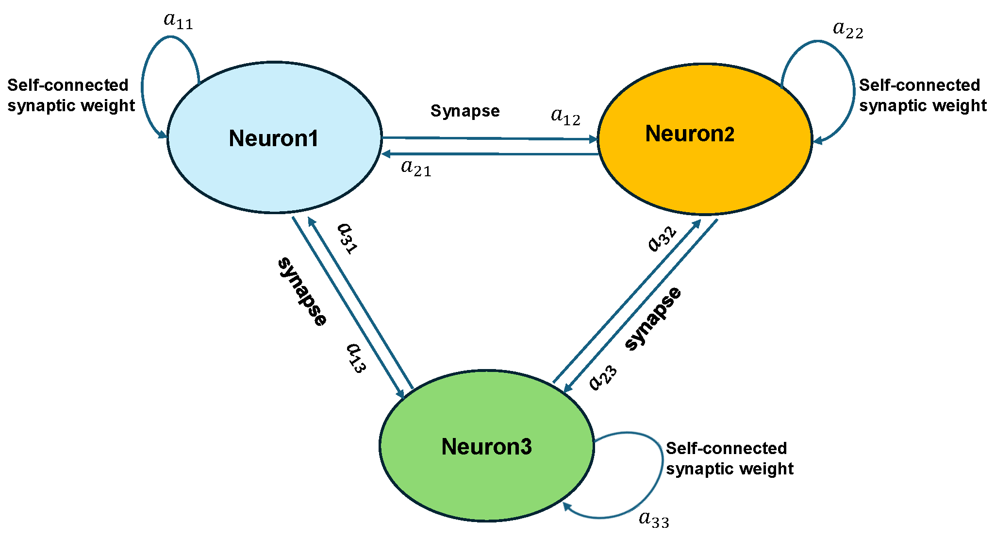
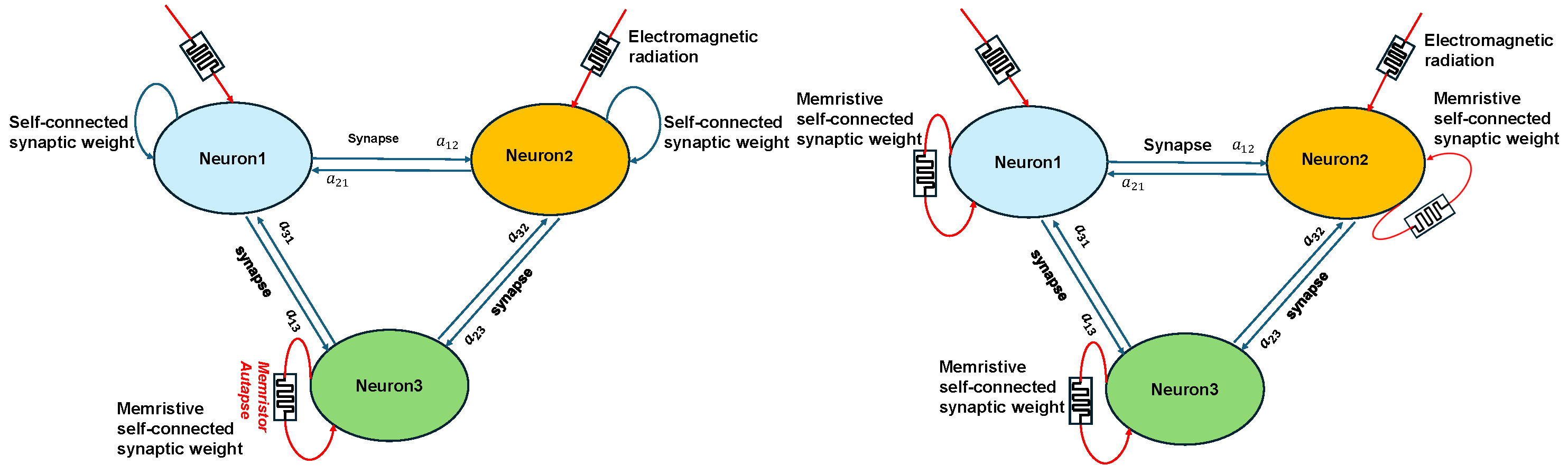
2. Formulation of Memristive-Based Neural Network Problem

We shall consider a network of m coupled neurons denoted by ${\mathcal{N}}_G=\{{\mathcal{N}}_i:i=1,2,\dots ,m\}$, where the network size $m\ge 2$ is a positive integer. Our model of a memristor-autapse-based neural network with external electromagnetic radiation can be depicted as in Figure 2.

In this paper, motivated by the above discussions (see Section 1), we introduce the following new fractional-order memristive neural network of coupled neurons, modeled by the following Caputo-fractional system, including the magnetic flux coupling (on each neuron ${\mathcal{N}}_i$ of the network, for $i=1,m$):

$$\begin{array}{c}{\displaystyle {\mathfrak{c}}_{\alpha }{\partial }_{0^{+}}^{\alpha }{\varphi }_i-div({\mathcal{K}}_f(\mathbf{x})\nabla {\varphi }_i)=F(\mathbf{x},{\varphi }_i)+\sigma u_i+\frac{{\xi }_h}{m}\sum _{j=1}^m{a}_{ij}(\mathbf{x},t)H_j({\varphi }_j)}\hfill \\ {\displaystyle +f_{ex}(\mathbf{x},t)-\kappa {\varphi }_i\Psi (w_i)+\frac{{\xi }_f}{m}{\mathcal{G}}_i({\varphi }_1,\dots ,{\varphi }_m),\mathrm{in}{\mathcal{Q}}_{\infty }}\hfill \\ {\displaystyle {\mathfrak{c}}_{\beta }{\partial }_{0^{+}}^{\alpha }{u}_i=a-b{u}_i-c_2{\varphi }_i^2+c_1{\varphi }_i,\mathrm{in}{\mathcal{Q}}_{\infty }}\hfill \\ {\displaystyle {\mathfrak{c}}_{\gamma }{\partial }_{0^{+}}^{\alpha }{w}_i-div({\mathcal{K}}_e(\mathbf{x})\nabla w_i)={\nu }_1{\varphi }_i-{\nu }_2{w}_i+g_{ex}(\mathbf{x},t)+\frac{{\xi }_e}{m}{\mathcal{G}}_i(w_1,\dots ,w_m),\mathrm{in}{\mathcal{Q}}_{\infty }}\hfill \end{array}$$

(1)

where ${\mathcal{Q}}_{\infty }=\Omega \times ]0,+\infty [$ and the spatial domain $\Omega$ is a bounded open subset and its boundary denoted by $\Gamma =\partial \Omega$ is locally Lipschitz continuous. Here, ${\partial }_{0^{+}}^{\alpha }$ denotes the forward Caputo fractional derivative with $\alpha$ a real value in $]0,1]$. The state variables ${\varphi }_i$, $u_i$, and $w_i$ describe, respectively, the membrane potential, the ionic variable, and the magnetic flux across the membrane of the i-th neuron ${\mathcal{N}}_i$, for $i=1,m$. The term F is the nonlinear activation operator. The functions $f_{ex}$ and $g_{ex}$ represent the external forcing current and the external field electromagnetic radiation, respectively. The parameters ${\xi }_h\ge 0$, ${\xi }_f\ge 0$, ${\xi }_e\ge 0$ are the coupling strength constants with ${\xi }_e{\xi }_f\ne 0$. The values a and $\sigma$ can be any nonzero number constants and all the parameters b, $c_1$, $c_2$, $\kappa$, ${\nu }_1$, and ${\nu }_2$ can be any positive constants.

The fractional parameter ${\mathfrak{c}}_{\alpha }$ is ${\mathfrak{c}}_{\alpha }={\kappa }_s{C}_{\alpha }>0$, where $C_{\alpha }$ is the membrane pseudo-capacitance per unit area and ${\kappa }_s$ is the surface area-to-volume ratio (homogenization parameter). The membrane is assumed to be passive, so the pseudo-capacitance $C_{\alpha }$ can be assumed to be constant. Moreover, since the electrical restitution curve (ERC) is affected by the action potential history through ionic memory, we have represented the memory via u (respectively, via w) by a time fractional-order dynamic term ${\mathfrak{c}}_{\beta }{\partial }_{0^{+}}^{\alpha }u$ (respectively, by ${\mathfrak{c}}_{\gamma }{\partial }_{0^{+}}^{\alpha }w$), where the positive parameters ${\mathfrak{c}}_{\beta }$ and ${\mathfrak{c}}_{\gamma }$ are assumed to be constants. The fractional parameters ${\mathfrak{c}}_{\alpha }$, ${\mathfrak{c}}_{\beta }$, and ${\mathfrak{c}}_{\gamma }$ depend on the fractional-order $\alpha$.

Remark 1.

According to the expression of the Caputo derivative, we can obtain that the unit for the dimension of ${\displaystyle \frac{{\mathfrak{c}}_{\alpha }}{\mathfrak{C}}}$ is $s^{\alpha -1}$, with s the unit for the dimension of time and $\mathfrak{C}$ the capacitance ${\mathfrak{c}}_{\alpha }$ for $\alpha =1$ (this result remains valid for ${\mathfrak{c}}_{\beta }$ and ${\mathfrak{c}}_{\gamma }$).

The functions $a_{ij}$, for $i,j=1,m$, represent the memristor’s synaptic connection weight coefficient (an example with three neurons is depicted in Figure 3).

The term ${\sum }_{j=1}^m{a}_{ij}(\mathbf{x},t)H_j({\varphi }_j)$ could be regarded as an emulation of a neurological disease, e.g., epileptic seizures, in which the nonlinear operators $H_j$ are some activation functions. We assume that (for $i,j=1,m$)

$$\begin{array}{c}{a}_{ij}\in L^{\infty }([0,+\infty )\times \overline{\Omega })\mathrm{with}{\underline{a}}_{ij}\le a_{ij}\le {\overline{a}}_{ij},\mathrm{a}.\mathrm{e}.,\mathrm{in}[0,+\infty )\times \overline{\Omega }\hfill \end{array}$$

(2)

where $({\overline{a}}_{ij},{\underline{a}}_{ij})$ are in ${IR}^2$, and we denote

$$\begin{array}{c}{\stackrel{s}{a}}_{ij}=max(\mid {\overline{a}}_{ij}\mid ,\mid {\underline{a}}_{ij}\mid )\mathrm{and}{\stackrel{d}{a}}_{ij}=\mid {\overline{a}}_{ij}-{\underline{a}}_{ij}\mid .\hfill \end{array}$$

(3)

The operator $\Psi =q_1{\Psi }_1+q_2{\Psi }_2$ is the memory conductance of the flux-controlled memristor, where ${\Psi }_1(w)={\delta }_1+{\eta }_{11}w+{\eta }_{12}{w}^2$, ${\Psi }_2(w)={\delta }_2+{\zeta }_{2}tanh(w)$, all the parameters ${\delta }_1$, ${\delta }_2$, ${\eta }_{11}$, ${\eta }_{12}$, ${\zeta }_2$ can be any positive constant, and $q_1{q}_2\ne 0$, with $q_k\ge 0$, for $k=1,2$. The magnetic flux coupling $\kappa \varphi \Psi (w)$ could be regarded as an additive induction current on the membrane and represents the dynamic effect of electromagnetic induction on neurological diseases (examples with three neurons are depicted in Figure 4). For simplicity, we can write $\Psi (w)=\delta +{\eta }_{1}w+{\eta }_2{w}^2+\zeta tanh(w)$, where $\delta =q_1{\delta }_1+q_2{\delta }_2$, ${\eta }_1=q_1{\eta }_{11}$, ${\eta }_2=q_1{\eta }_{12}$, and $\zeta =q_2{\zeta }_2$.

The operator ${\mathcal{G}}_i$, which contains the information of network topology, is defined by (for $i=1,m$)

$${\displaystyle {\mathcal{G}}_i(v_1,\dots ,v_m)=\sum _{k=1,k\ne i}^m{G}_{ik}(v_k-v_i)}$$

(4)

with the coupling (or connectivity) matrix $\mathbf{G}={(G_{ij})}_{1\le i,j\le m}$ ($-\mathbf{G}$ is called the Laplacian matrix of the graph), in which $G_{ij}$ are the coefficients of connection from the i-th to the j-th neuron, satisfying the assumption

(HG) 

$G_{ik}\ge 0$ for $i\ne k$ and ${\displaystyle G_{ii}=-\sum _{k=1,k\ne i}^m{G}_{ik}}$, i.e., the matrix $\mathbf{G}$ has vanishing row and column sums and non-negative off-diagonal elements.

Then, ${\mathcal{G}}_i(v_1,\dots ,v_m)$ can be written as ${\displaystyle {\mathcal{G}}_i(v_1,\dots ,v_m)=\sum _{k=1}^m{G}_{ik}{v}_k.}$

In graph theory, the Laplacian matrix $-\mathbf{G}$, also called the graph Laplacian or Kirchhoff matrix, defines the graph topology with m the number of vertices/nodes ${\mathcal{N}}_i$ in graph $\mathbb{G}({\mathcal{N}}_G,{\mathcal{E}}_G)$ (with ${\mathcal{N}}_G$ set of vertices and ${\mathcal{E}}_G$ set of edges/links). The diagonal matrix $\mathbf{D}=-diag(G_{11},\dots ,G_{mm})$ is called the degree matrix of graph and $\mathbf{A}:=\mathbf{D}+\mathbf{G}$ is called the adjacency matrix of the graph.

The state variable $({\varphi }_i,u_i,w_i)$, for $i=1,m$ in this network, is coupled with the other neurons $\{{\mathcal{N}}_j:j\ne i\}$ in the network through the state equation by ${\mathcal{G}}_i$ and/or through the boundary conditions as follows (fully connected network on boundary):

$$\begin{array}{c}{\displaystyle \left({\mathcal{K}}_f.\nabla {\varphi }_i\right)·\mathbf{n}-\frac{p_f}{m}\sum _{k=1,m}({\varphi }_k-{\varphi }_i)=0,\mathrm{on}\Gamma ,}\hfill \\ {\displaystyle \left({\mathcal{K}}_e.\nabla w_i\right)·\mathbf{n}-\frac{p_e}{m}\sum _{k=1,m}(w_k-w_i)=0,\mathrm{on}\Gamma .}\hfill \end{array}$$

(5)

where $\mathbf{n}$ is the outward normal to $\Gamma$ and $p_f>0$, $p_e>0$ are the coupling strength constants on boundary. The tensors ${\mathcal{K}}_f$ and ${\mathcal{K}}_e$ are the effective diffusion tensors that describe the heterogeneity of brain tissue and local anisotropy of cell diffusion.

The initial conditions of (1) to be specified will be denoted by (for $i=1,m$)

$$\begin{array}{c}({\varphi }_i(0),u_i(0),w_i(0))=({\varphi }_{0i},u_{0i},w_{0i}),\mathrm{on}\Omega .\hfill \end{array}$$

(6)

The rest of the paper is organized as follows. In the next section, we give some preliminary results useful in the sequel. In Section 4, we shall prove the existence, stability, and uniqueness of weak solutions of the derived model, under some hypotheses for data and some regularity of nonlinear operators. An important feature of the uniqueness of the solution is the semiflow physical property of the system; starting the system at time $t_0$, letting it run until time $s=t_0+\tau$, and then restarting it and letting it run from time s to the final time of $T_f$ amounts to running the system directly from time $t_0$ to final time $T_f$. In Section 5, the existence of an absorbing set in state spaces for the system is discussed, an estimate of the solutions is derived when time is large enough, and then the dissipative dynamics result, with absorbing sets, is proved. In Section 6, synchronization phenomena are discussed and some Mittag–Leffler synchronization criteria for such complex dynamical networks are established in different situations. Precisely, some sufficient conditions for the synchronization are obtained first for the complete (or identical) synchronization (which refers to the process by which two or more identical dynamical systems adjust their motion in order to converge to the same dynamical state as time approaches infinity) problem and then for the master–slave synchronization problem via appropriate pinning feedback controllers and adaptive controllers. In Section 7, conclusions are discussed. In Appendix A, the full proof of well-posedness of the derived system is shown, and in Appendix B, a brief introduction to some definitions and basic results in fractional calculus in the Rieman–Liouville sense and Caputo sense is given.

3. Assumptions, Notations, and Some Fundamental Inequalities

Some basic definitions, notations, fundamental inequalities, and preliminary lemmas are introduced and other results are developed.

Let $\mho \subset {IR}^d$, $d\ge 1$, be an open and bounded set with a smooth boundary and ${\mho }_T=\mho \times (0,T)$. We use the standard notation for Sobolev spaces (see [59]), denoting the norm of $W^{q,p}(\mho )$ ($q\in IN$, $p\in [1,\infty ]$) by ${\displaystyle {\Vert .\Vert }_{W^{q,p}}}$. In the special case $p=2$, we use $H^q(\mho )$ instead of $W^{q,2}(\mho )$. The duality pairing of a Banach space X with its dual space $X^{\prime }$ is given by ${\langle .,.\rangle }_{X^{\prime },X}$. For a Hilbert space Y, the inner product is denoted by ${(.,.)}_Y$ and the inner product in $L^2(\Omega )$ is denoted by $(.,.)$. For any pair of real numbers $r,s\ge 0$, we introduce the Sobolev space $H^{r,s}({\mho }_T)=L^2(0,T;H^r(\mho ))\cap H^s(0,T;L^2(\mho )),$ which is a Hilbert space normed by ${\displaystyle {\left({\Vert v\Vert }_{L^2(0,T;H^r(\mho ))}^2+{\Vert v\Vert }_{H^s(0,T;L^2(\mho ))}^2\right)}^{1/2}}$, where space $H^s(0,T;L^2(\mho ))$ denotes the Sobolev space of order s of functions defined on $(0,T)$ and taking values in $L^2(\mho )$, and defined by interpolation as $H^s(0,T;L^2(\mho ))={[H^q(0,T,L^2(\mho )),L^2({\mho }_T)]}_{\theta }$, for $s=(1-\theta )q$ with $\theta \in (0,1)$ and $q\in IN$, and $H^q(0,T;L^2(\mho ))=\left\{v\in L^2({\mho }_T)|\frac{{\partial }^{j}v}{\partial t^j}\in L^2({\mho }_T),\mathrm{for}1\le j\le q\right\}$.

We now recall the following Poincaré–Steklov inequalities (see, e.g., [60]):

Lemma 1.

(Poincaré–Steklov inequality) Assume that ℧ is a bounded connected open subset of ${IR}^d$ with a sufficiently regular boundary $\partial \mho$ (e.g., a Lipschitz boundary). Then,

$$C_{PS}^2{(\zeta )\Vert v\Vert }_{L^2(\mho )}^2\le {\ell }_{\mho }^2{(\Vert \nabla v\Vert }_{L^2(\mho )}^2+{\zeta \Vert v\Vert }_{L^2(\partial \mho )}^2),\forall v\in H^1(\mho ).$$

 where ${\ell }_{\mho }:=diam(\mho )>0$ and $C_{PS}^2>0$ is the smallest eigenvalue of the Laplacian supplemented with the Robin boundary condition $\zeta v+\mathbf{n}.\nabla v=0$ on $\partial \mho$ (with $\zeta >0$ any positive constant).

Lemma 2.

(Extended Poincaré–Steklov inequality). Assume that $q\in [1,\infty )$ and that ℧ is a bounded connected open subset of ${IR}^d$ with a sufficiently regular boundary $\partial \mho$ (e.g., a Lipschitz boundary). Let R be a bounded linear form on $W^{1,q}(\mho )$ whose restriction on constant functions is not zero. Then, there exists a Poincaré–Steklov constant ${\widehat{C}}_{PS;q}>0$ such that ${\displaystyle {\widehat{C}}_{PS;q}{\Vert v\Vert }_{L^q(\mho )}\le {\ell }_{\mho }{\Vert \nabla v\Vert }_{L^q(\mho )}+\mid R(v)\mid ,\forall v\in W^{1,q}(\mho ).}$

Remark 2.

Let q be a nonnegative integer and ℧ be a bounded connected open subset of ${IR}^d$ with a sufficiently regular boundary $\partial \mho$. We have the following results (see, e.g., [59]):

(i) $H^1(\mho )\subset L^p(\mho )$, $\forall p\in [1,\frac{2d}{d-2q}]$, with continuous embedding (with the exception that if $2q=d$, then $p\in [1,+\infty [$ and if $2q>d$, then $p\in [1,+\infty ]$ ).

(ii) (Gagliardo–Nirenberg inequalities) There exists $C_{\mho ,q,\theta }>0$ such that

$${\Vert v\Vert }_{L^p(\mho )}\le C_{\mho ,q,\theta }{(\Vert \nabla v\Vert }_{L^2(\mho )}^{\theta }{\Vert v\Vert }_{L^q(\mho )}^{(1-\theta )}+{\Vert v\Vert }_{L^q(\mho )}),\forall v\in H^1(\mho )\times L^q(\mho ),$$

 where $0\le \theta \le 1$, $q\ge 1$, and $p>0$ such that $\frac{d}{p}=\theta (\frac{d}{2}-1)+(1-\theta )\frac{d}{q}$ (with the exception that if $1-\frac{d}{2}$ is a nonnegative integer, $0\le \theta <1$).

Definition 1

(see, e.g., [61]). A real valued function $\mathcal{H}$ defined on $D\times {IR}^q$, $q\ge 1$, is a Carathéodory function iff $\mathcal{H}(.;\mathbf{v})$ is measurable for all $\mathbf{v}\in {IR}^q$ and $\mathcal{H}(y;.)$ is continuous for almost all $y\in D$.

Our study involves the following fundamental inequalities, which are repeated here for review:

• (i) Hölder’s inequality: ${\displaystyle {\int }_D{\Pi }_{i=1,k}{f}_{i}d\mathbf{x}\le {\Pi }_{i=1,k}{\Vert f_i\Vert }_{L^{q_i}(D)}}$, where ${\displaystyle \sum _{1\le i\le k}\frac{1}{q_i}=1.}$
• (ii) Young’s inequality ($\forall a,b>0$ and $ϵ>0$): ${\displaystyle ab\le \frac{ϵ}{p}{a}^p+\frac{{ϵ}^{-q/p}}{q}{b}^q,forp,q\in ]1,+\infty [and\frac{1}{p}+\frac{1}{q}=1.}$
• (iii) Minkowski’s integral inequality ($\mathrm{for}p\in ]1,+\infty [\mathrm{and}t>0$):

  $$\begin{array}{c}{\displaystyle {\left[{\int }_{\Omega }{\left({\int }_0^t\mid f(\mathbf{x},s)\mid ds\right)}^{p}d\mathbf{x}\right]}^{1/p}\le {\int }_0^t{\left({\int }_{\Omega }\mid f(\mathbf{x},s){\mid }^{p}d\mathbf{x}\right)}^{1/p}ds.}\hfill \end{array}$$

Finally, we denote by $\mid \mho \mid$ the Lebesgue measure of ℧, by $sgn(x)$ the sign of the scalar x, and by $\mathfrak{L}(A;B)$ the set of linear and continuous operators from a vector space A into a vector space B. The operator ${\mathcal{R}}^{\ast }$ stands for the adjoint to linear operator $\mathcal{R}$ between Banach spaces.

From now on, we assume that the following assumptions hold for nonlinear operators, matrix coupling, and tensor functions appearing in our model on $\Omega$.

First we introduce the following spaces: ${\displaystyle \mathbb{H}=L^2(\Omega )}$ and ${\displaystyle \mathbb{V}=H^1(\Omega )}$ (endowed with their usual norms). We will denote by ${\displaystyle {\mathbb{V}}^{\prime }}$ the dual of ${\displaystyle \mathbb{V}}$. We have the following continuous embeddings ($p^{\prime }$ is such that ${\displaystyle \frac{1}{p^{\prime }}+\frac{1}{p}=1}$):

$$\begin{array}{c}\mathbb{V}\subset \mathbb{H}\subset {\mathbb{V}}^{\prime }\mathrm{and}\mathbb{V}\subset L^p(\Omega )\subset \mathbb{H}\equiv {\left(\mathbb{H}\right)}^{\prime }\subset L^{p^{\prime }}(\Omega )\subset {\mathbb{V}}^{\prime }\hfill \end{array}$$

(7)

and the injection $\mathbb{V}\subset \mathbb{H}$ is compact, where $p\ge 2$ if $d=2$ and $2\le p\le 6$ if $d=3$.

For tensor functions, we assume that the following assumptions hold.

(H1) 

We assume that the conductivity tensor functions ${\mathcal{K}}_{\theta }\in W^{1,\infty }(\overline{\Omega })$, $\theta \in \{e,f\}$, are symmetric, positive definite matrix functions and that they are uniformly elliptic, i.e., there exist constants $0<d_f\le r_f$ and $0<d_e\le r_e$ such that ($\forall v\in {IR}^n$)

$$\begin{array}{c}{\displaystyle d_f{\parallel v\parallel }^2\le v^T{\mathcal{K}}_{f}v\le r_f{\parallel v\parallel }^2\mathrm{and}{d}_e{\parallel v\parallel }^2\le v^T{\mathcal{K}}_{e}v\le r_e{\parallel v\parallel }^2\mathrm{in}\overline{\Omega }.}\hfill \end{array}$$

(8)

The operators F and ${(H_i)}_{i=1,m}$, which describe behavior of the system, are supposed to satisfy the following assumptions.

(H2) 

The operators F and ${(H_i)}_{i=1,m}$ are Carathéodory functions from $\Omega \times IR$ into $IR$. Furthermore, the following requirements hold.

  ${(H2)}_1$

The nonlinear scalar activation function $F\in C^1(\Omega \times IR)$, which can be taken as $F=F_1+F_2$ with $F_1$ as a decreasing function on the second variable, satisfies ($\forall (x,v)\in \Omega \times IR$):

 (i)

$F(x,v)v\le -\lambda \mid v{\mid }^4+{\rho }_0(x)$;

 (ii)

$\mid F(x,v)\mid \le {\alpha }_1\mid v{\mid }^3+{\rho }_1(x)$;

 (iii)

$\mid \frac{\partial F}{\partial v}(x,v)\mid \le {\alpha }_2\mid v{\mid }^2+{\rho }_2(x)$ and $\frac{\partial F}{\partial v}(x,v)\le -{\alpha }_3\mid v{\mid }^2+\beta$;

 (iv)

$\mid F_2(x,v)\mid \le {\alpha }_4\mid v{\mid }^2+{\rho }_3(x)$;

 (v)

$\mid {\mathcal{E}}_F(x,v)\mid \le {\alpha }_5\mid v{\mid }^4+{\rho }_4(x)$ and ${\mathcal{E}}_F(x,v)\le -{\alpha }_6\mid v{\mid }^4+{\alpha }_7\mid v{\mid }^2+{\alpha }_8$.

$\lambda$, $\beta$, and ${\alpha }_i$, for $i=1,8$, are positive constants, ${\rho }_i\in L^2(\Omega )$, for $i=0,4$, are given functions, and ${\mathcal{E}}_F$ is the primitive function of $F_1$.

  ${(H2)}_2$

The nonlinear scalar activation functions $H_i$ are bounded with $H_i(0)=0$ and satisfy $l_i$-Lipschitz condition, i.e.,

 (vi)

$\mid H_i(u)\mid \le M_i$ and $\mid H_i(u)-H_i(v)\mid \le l_i\mid u-v\mid$, $\forall (u,v)\in {IR}^2$, with $l_i>0$ and $M_i>0$.

For the operators ${({\mathcal{G}}_i)}_{i=1,m}$, which are defined from the matrix coupling G, we introduce first the following notations: the matrix $\mathbf{S}={({ϵ}_{ij})}_{1\le i,j\le m}$, where ${ϵ}_{ij}={ϵ}_{ji}=\frac{1}{2}(G_{ij}+G_{ji})$ and the matrix $\mathbf{A}={({\delta }_{ij})}_{1\le i,j\le m}$, where ${\delta }_{ij}=-{\delta }_{ij}=\frac{1}{2}(G_{ij}-G_{ji})$, for $i\ne j$. Then, the matrix $\mathbf{S}$ is symmetric, the matrix $\mathbf{A}$ is antisymmetric, and $\mathbf{G}$ can be represented uniquely as $\mathbf{G}=\mathbf{S}+\mathbf{A}$. It is evident that both $\mathbf{S}$ and $\mathbf{A}$ have zero row sums (i.e., ${\displaystyle \sum _{k=1}^m{ϵ}_{jk}=0}$ and ${\displaystyle \sum _{k=1}^m{\delta }_{jk}=0}$) and ${\displaystyle 2{\delta }_{ii}=\sum _{k=1}^m{G}_{ki}}$. Then, we can now derive the following two lemmas.

Lemma 3.

For $(\varphi ,w,u)$ in $L^4(\Omega )\times L^2(\Omega )\times L^2(\Omega )$ and $(f_{ex},g_{ex},{\rho }_0)\in {(L^2(\Omega ))}^3$, we have the following inequalities:

$$\begin{array}{c}{\displaystyle (i)-\kappa {\int }_{\Omega }\mid \varphi {\mid }^2(\delta +{\eta }_{1}w+{\eta }_2{(w)}^2+\zeta tanh(w))d\mathbf{x}\le {\theta }_w{\Vert \varphi \Vert }_{L^2(\Omega )}^2,}\hfill \\ {\displaystyle (\mathit{ii}){\int }_{\Omega }F(\mathbf{x},\varphi )\varphi d\mathbf{x}+\sigma {\int }_{\Omega }u\varphi d\mathbf{x}+{\int }_{\Omega }{f}_{ex}\varphi d\mathbf{x}\le -\frac{\lambda }{2}{\int }_{\Omega }\mid \varphi {\mid }^{4}d\mathbf{x}+\frac{\upsilon }{2}{\Vert u\Vert }_{L^2(\Omega )}^2}\hfill \\ {\displaystyle +\frac{1}{2\lambda }\Vert f_{ex}{\Vert }_{L^2(\Omega )}^2+\mid \Omega \mid (\Vert {\rho }_0{\Vert }_{L^2(\Omega )}+\frac{1}{2\lambda }{(\frac{{\sigma }^2}{2\upsilon }+\frac{\lambda }{2})}^2),}\hfill \\ {\displaystyle (\mathit{iii})c_1{\int }_{\Omega }\varphi ud\mathbf{x}-c_2{\int }_{\Omega }\mid \varphi {\mid }^{2}ud\mathbf{x}+a{\int }_{\Omega }ud\mathbf{x}-b{\Vert u\Vert }_{L^2(\Omega )}^2}\hfill \\ {\displaystyle \le -\frac{5b}{8}{\Vert u\Vert }_{L^2(\Omega )}^2+\frac{2c_1^2}{b}{\Vert \varphi \Vert }_{L^2(\Omega )}^2+\frac{2a^2\mid \Omega \mid }{b}+\frac{2c_2^2}{b}{\Vert \varphi \Vert }_{L^4(\Omega )}^4,}\hfill \end{array}$$

(9)

 where ${\theta }_0=\frac{{\eta }_1}{2{\eta }_2}$, ${\theta }_w=\kappa ({\eta }_2{\theta }_0^2+\zeta -\delta )$ and $\upsilon >0$ (υ is any positive constant, to be chosen appropriately).

Proof. 

Since $\mid tanh(w)\mid \le 1$, we have (according to assumption $(\mathbf{H}\mathbf{2})$)

$$\begin{array}{c}{\displaystyle -\kappa {\int }_{\Omega }\mid \varphi {\mid }^2(\delta +{\eta }_{1}w+{\eta }_2{(w)}^2+\zeta tanh(w))d\mathbf{x}}\hfill \\ {\displaystyle \le \kappa (\zeta -\delta ){\int }_{\Omega }\mid \varphi {\mid }^{2}d\mathbf{x}-\kappa {\eta }_2{\int }_{\Omega }\mid \varphi {\mid }^2({(w+{\theta }_0)}^2-{\theta }_0^2)d\mathbf{x}}\hfill \\ {\displaystyle \le {\theta }_w{\Vert \varphi \Vert }_{L^2(\Omega )}^2,}\hfill \\ {\displaystyle {\int }_{\Omega }F(\mathbf{x},\varphi )\varphi d\mathbf{x}+\sigma {\int }_{\Omega }u\varphi d\mathbf{x}+{\int }_{\Omega }{f}_{ex}\varphi d\mathbf{x}}\hfill \\ {\displaystyle \le -\lambda {\int }_{\Omega }\mid \varphi {\mid }^{4}d\mathbf{x}+\sigma {\int }_{\Omega }u\varphi d\mathbf{x}+{\int }_{\Omega }{f}_{ex}\varphi d\mathbf{x}+{\int }_{\Omega }{\rho }_{0}d\mathbf{x}}\hfill \\ {\displaystyle \le -\lambda {\int }_{\Omega }\mid \varphi {\mid }^{4}d\mathbf{x}+\frac{\upsilon }{2}{\Vert u\Vert }_{L^2(\Omega )}^2+(\frac{{\sigma }^2}{2\upsilon }+\frac{\lambda }{2}){\Vert \varphi \Vert }_{L^2(\Omega )}^2+\frac{1}{2\lambda }\Vert f_{ex}{\Vert }_{L^2(\Omega )}^2+\mid \Omega \mid {\Vert {\rho }_0\Vert }_{L^2(\Omega )}}\hfill \\ {\displaystyle \le -\frac{\lambda }{2}{\int }_{\Omega }\mid \varphi {\mid }^{4}d\mathbf{x}+\frac{\upsilon }{2}{\Vert u\Vert }_{L^2(\Omega )}^2+\frac{1}{2\lambda }\Vert f_{ex}{\Vert }_{L^2(\Omega )}^2+\mid \Omega \mid (\Vert {\rho }_0{\Vert }_{L^2(\Omega )}+\frac{1}{2\lambda }{(\frac{{\sigma }^2}{2\upsilon }+\frac{\lambda }{2})}^2)}\hfill \end{array}$$

and

$$\begin{array}{c}{\displaystyle c_1{\int }_{\Omega }\varphi ud\mathbf{x}-c_2{\int }_{\Omega }\mid \varphi {\mid }^{2}ud\mathbf{x}+a{\int }_{\Omega }ud\mathbf{x}-b{\Vert u\Vert }_{L^2(\Omega )}^2}\hfill \\ {\displaystyle \le -\frac{5b}{8}{\Vert u\Vert }_{L^2(\Omega )}^2+\frac{2c_1^2}{b}{\Vert \varphi \Vert }_{L^2(\Omega )}^2+\frac{2a^2\mid \Omega \mid }{b}+\frac{2c_2^2}{b}{\int }_{\Omega }\mid \varphi {\mid }^{4}d\mathbf{x}.}\hfill \end{array}$$

This completes the proof. □

The estimates of the previous lemma are needed to construct a priori estimates (to establish the existence result).

Lemma 4.

For all ${(v_i)}_{i=1,m}\in {IR}^m$, we have the following relations (with ${\psi }_{ij}=v_j-v_i$ for $1\le i,j\le m$).

${\displaystyle (i)\sum _{\begin{array}{c}1\le i\le m\\ 1\le k\le m\end{array}}{G}_{ik}{v}_k{v}_i=\frac{-1}{2}\sum _{i,k=1;k\ne i}^m{G}_{ik}{(v_k-v_i)}^2+\sum _{k=1}^m{\delta }_{kk}{v}_k^2}$,

$\begin{array}{c}{\displaystyle (ii)\sum _{\begin{array}{c}1\le i,j\le m\\ 1\le k\le m\end{array}}(G_{jk}-G_{ik})v_k{\psi }_{ij}=-m\sum _{1\le k,j\le m}{ϵ}_{jk}{\psi }_{jk}^2+2\sum _{1\le i,j\le m}{\delta }_{jj}{\psi }_{ij}^2}\hfill \\ {\displaystyle =-m\sum _{1\le k,j\le m}{ϵ}_{jk}{\psi }_{jk}^2+m\sum _{1\le i,j\le m}{\mu }_{ij}{\psi }_{ij}^2,\mathrm{with}{\mu }_{ij}=\frac{{\delta }_{ii}+{\delta }_{jj}}{m}.}\hfill \end{array}$

Proof. 

Since ${\sum }_{k=1}^m{G}_{ik}=0$, we can deduce that

$$\sum _{i,k=1;k\ne i}^m{G}_{ik}{(v_k-v_i)}^2=\sum _{k=1}^m(\sum _{i=1}^m{G}_{ik})v_k^2-2\sum _{i,k=1}^m{G}_{ik}{v}_k{v}_i=2\sum _{k=1}^m{\delta }_{kk}{v}_k^2-2\sum _{i,k=1}^m{G}_{ik}{v}_k{v}_i$$

and then the relation (i). For the relation (ii), we have (we proceed in a similar way as in [62])

$$\begin{array}{c}{\displaystyle \sum _{\begin{array}{c}1\le i,j\le m\\ 1\le k\le m\end{array}}(G_{jk}-G_{ik})v_k{\psi }_{ij}=-\sum _{\begin{array}{c}1\le i,j\le m\\ 1\le k\le m\end{array}}({ϵ}_{ik}{\psi }_{ik}+{\delta }_{ik}{\psi }_{ik}-{ϵ}_{jk}{\psi }_{jk}-{\delta }_{jk}{\psi }_{jk}){\psi }_{ij}}\hfill \\ {\displaystyle =\sum _{\begin{array}{c}1\le i,j\le m\\ 1\le k\le m\end{array}}({ϵ}_{jk}{\psi }_{jk}-{ϵ}_{ik}{\psi }_{ik}){\psi }_{ij}+\sum _{\begin{array}{c}1\le i,j\le m\\ 1\le k\le m\end{array}}({\delta }_{jk}{\psi }_{jk}-{\delta }_{ik}{\psi }_{ik}){\psi }_{ij}=I+II.}\hfill \end{array}$$

Since ${\displaystyle {\psi }_{jk}={\psi }_{ji}+{\psi }_{ik}}$ and ${\displaystyle \sum _{k=1}^m{\delta }_{jk}=0}$, we can deduce that

$$\begin{array}{c}{\displaystyle II=\sum _{\begin{array}{c}1\le i,j\le m\\ 1\le k\le m\end{array}}({\delta }_{jk}{\psi }_{jk}-{\delta }_{ik}{\psi }_{ik}){\psi }_{ij}=\sum _{k=1}^m\sum _{i=1}^m\sum _{j=1}^m({\delta }_{jk}{\psi }_{jk}{\psi }_{ij})-\sum _{k=1}^m\sum _{i=1}^m\sum _{j=1}^m({\delta }_{jk}{\psi }_{jk}{\psi }_{ji})}\hfill \\ {\displaystyle =2\sum _{\begin{array}{c}1\le i,j\le m\\ 1\le k\le m\end{array}}{\delta }_{jk}{\psi }_{jk}{\psi }_{ij}=2\sum _{1\le i,j\le m}{\delta }_{jj}{\psi }_{ij}^2+2\sum _{i=1}^m(\sum _{j,k=1;k\ne j}^m{\psi }_{ij}{\delta }_{jk}{\psi }_{ik}).}\hfill \end{array}$$

We can deduce that ${\displaystyle \sum _{j,k=1;k\ne j}^m{\psi }_{ij}{\delta }_{jk}{\psi }_{ik}=\sum _{1\le j<k\le m}{\psi }_{ij}({\delta }_{jk}+{\delta }_{kj}){\psi }_{ik}=0}$ (since ${\displaystyle {\delta }_{jk}+{\delta }_{kj}=0}$), and then ${\displaystyle II=2\sum _{1\le i,j\le m}{\delta }_{jj}{\psi }_{ij}^2=m\sum _{1\le i,j\le m}{\mu }_{ij}{\psi }_{ij}^2}$, with ${\displaystyle {\mu }_{ij}=\frac{{\delta }_{ii}+{\delta }_{jj}}{m}}$, for $1\le i,j\le m$. For the term I, we have that

$$\begin{array}{c}{\displaystyle I=\sum _{\begin{array}{c}1\le i,j\le m\\ 1\le k\le m\end{array}}({ϵ}_{jk}{\psi }_{jk}-{ϵ}_{ik}{\psi }_{ik}){\psi }_{ij}=\sum _{\begin{array}{c}1\le i,j\le m\\ 1\le k\le m\end{array}}{ϵ}_{jk}{\psi }_{jk}{\psi }_{ij}-\sum _{\begin{array}{c}1\le i,j\le m\\ 1\le k\le m\end{array}}{ϵ}_{jk}{\psi }_{jk}{\psi }_{ji}}\hfill \\ {\displaystyle =2\sum _{\begin{array}{c}1\le i,j\le m\\ 1\le k\le m\end{array}}({ϵ}_{jk}{\psi }_{jk}{\psi }_{ij})}\hfill \end{array}$$

(10)

and then

$$\begin{array}{c}{\displaystyle I=\sum _{\begin{array}{c}1\le i,j\le m\\ 1\le k\le m\end{array}}{ϵ}_{jk}{({\psi }_{jk}+{\psi }_{ij})}^2-\sum _{\begin{array}{c}1\le i,j\le m\\ 1\le k\le m\end{array}}{ϵ}_{jk}({\psi }_{jk}^2+{\psi }_{ij}^2)}\hfill \\ {\displaystyle =\sum _{1\le i,k\le m}(\sum _{1\le j\le m}{ϵ}_{jk}){\psi }_{ik}^2-\sum _{\begin{array}{c}1\le i,j\le m\\ 1\le k\le m\end{array}}{ϵ}_{jk}{\psi }_{jk}^2-\sum _{1\le i,j\le m}(\sum _{1\le k\le m}{ϵ}_{jk}){\psi }_{ij}^2}\hfill \\ {\displaystyle =-m\sum _{1\le j,k\le m}{ϵ}_{jk}{\psi }_{jk}^2(\mathrm{since}\mathbf{S}\mathrm{is}\mathrm{symmetric}\mathrm{and}\mathrm{has}\mathrm{zero}\mathrm{row}\mathrm{sums}).}\hfill \end{array}$$

(11)

This completes the proof. □

Remark 3.

(a) If ${\sum }_{k=1}^m{G}_{ki}=0$ then ${\delta }_{ii}=0$ (for all $i=1,m$) and consequently ${\displaystyle \sum _{1\le i,j\le m}{\delta }_{jj}{\psi }_{ij}^2=0}$ (with ${\psi }_{ij}=(v_j-v_i)$) and ${\displaystyle \sum _{i=1}^m{\delta }_{ii}{v}_i^2=0}$ (in Lemma 4).

(b) The matrix ${({\mu }_{ij})}_{i,j}$ is symmetric and satisfies ${\sum }_{1\le i,j\le m}{\mu }_{ij}=0$.

Remark 4.

Let $\mathbb{A}$ be an arbitrary antisymmetric matrix. Then, for any vector w, we have $w^t\mathbb{A}w=0.$

To end this section, we give the following lemmas and definitions. From, e.g., [63,64], we can deduce, respectively, the following Lemmas.

Lemma 5.

(A generalized Gronwall’s inequality) Assume $\gamma >0$, h is a nonnegative function locally integrable on $(0,T)$ (some $T\le +\infty$) and b is a nonnegative, bounded, nondecreasing continuous function defined on $[0,T)$. Let f be a nonnegative and locally integrable function on $(0,T)$ with, for $t\in (0,T)$, $f(t)\le h(t)+b(t)I_{0^{+}}^{\gamma }\left[f\right](t).$ Then (for $t\in (0,T)$), ${\displaystyle f(t)\le h(t)+{\int }_0^t\sum _{k=1}^{\infty }h(\tau ){(t-\tau )}^{k\gamma -1}\frac{{(b(t))}^k}{\Gamma (k\gamma )}d\tau .}$ If, in addition, h is a nondecreasing function on $(0,T)$, then $f(t)\le h(t)E_{\gamma ,1}(b(t)t^{\gamma }).$

The used function ${\displaystyle E_{{\theta }_1,{\theta }_2}}$ is the classical two-parametric Mittag–Leffler function (usually denoted by ${\displaystyle E_{{\theta }_1}}$ if ${\theta }_2=1$), which is defined by ${\displaystyle E_{{\theta }_1,{\theta }_2}(z)=\sum _{k=0}^{\infty }\frac{1}{\Gamma (k{\theta }_1+{\theta }_2)}{z}^k.}$ The function $E_{{\theta }_1,{\theta }_2}$ is an entire function of the variable z for any ${\theta }_1,{\theta }_2\in ℂ$, $Re({\theta }_1)>0$.

Lemma 6.

Let ω be a locally integrable nonnegative function on $[0,+\infty )$ such that ${\partial }_{0^{+}}^{\alpha }\omega (t)+\lambda \omega (t)\le R$. Then, we have $\omega (t)\le \omega (0)E_{\alpha ,1}(-\lambda t^{\alpha })+R{t}^{\alpha }{E}_{\alpha ,\alpha +1}(-\lambda t^{\alpha })=\omega (0)E_{\alpha ,1}(-\lambda t^{\alpha })+R(1-E_{\alpha ,1}(-\lambda t^{\alpha })).$

The invertibility of $f(t)=E_{\alpha ,\beta }(-t),t>0$ follows from the complete monotonicity property of $E_{\alpha ,\beta }$. As shown in [65], this function is completely monotone if and only if $0<\alpha \le 1$ and $\beta \ge \alpha$. Since $E_{\alpha ,\beta }(0)=\Gamma {(\beta )}^{-1}$ and ${\displaystyle \underset{t⟶+\infty }{lim}{E}_{\alpha ,\beta }(-t)=0}$, then the inverse function $g=-L_{\alpha ,\beta }$ of f, is the function $g:(0,\Gamma {(\beta )}^{-1}]⟶[0,\infty )$ ($0<\alpha \le 1$ and $\beta \ge \alpha$).

Definition 2

(see, e.g., [66]). The initial-boundary value problem (1)–(6) is called dissipative in a Banach space $\mathbb{L}(\Omega )$ if there is a bounded set, in $\mathbb{L}(\Omega )$, $K_S=B(0,r)$ for some positive constants $r>0$ such that for any bounded subsets $K_I$ (of $\mathbb{L}(\Omega )$) and all initial data ${({\varphi }_{0i},u_{0i},w_{0i})}_{i=1,m}$ belonging to $K_I$, there exists a time $T_K$, depending on $K_I$, such that the corresponding solution ${({\varphi }_i(t),u_i(t),w_i(t))}_{i=1,m}$ is contained in $K_S$ for all $t\ge T_K$. The set $K_S$ is called an absorbing set and r is called a radius of dissipativity.

Remark 5.

(i) We can also express the previous definition as follows. For any bounded set $K_I$, there exists a finite time $T_K$ such that any solution started with initial condition in $K_I$ remains within the bounded ball $K_S$ for all time $t\ge T_K$.

(ii) The study of dissipative dynamics opens the way to the analysis of the synchronization problem.

Definition 3

(see, e.g., [67]). The initial-boundary value problem (1)–(6) is (locally) complete synchronized if

$${\displaystyle \underset{t⟶+\infty }{lim}(\Vert {\varphi }_i-{\varphi }_j{\Vert }_{L^2(\Omega )}+\Vert u_i-u_j{\Vert }_{L^2(\Omega )}+\Vert w_i-w_j{\Vert }_{L^2(\Omega )})=0,\forall i,j=1,m,}$$

 whenever the initial state belongs to an appropriate bounded open set.

Definition 4.

The initial-boundary value problem (1)–(6) is locally complete Mittag–Leffler synchronized if there exist $X^{\ast }>0$ and ${\lambda }^{\ast }>0$ such that for any $t>t^{\ast }$ ($\forall i,j=1,m$),

$$(\Vert {\varphi }_i-{\varphi }_j{\Vert }_{L^2(\Omega )}^2+\Vert u_i-u_j{\Vert }_{L^2(\Omega )}^2+\Vert w_i-w_j{\Vert }_{L^2(\Omega )}^2)(t)\le X^{\ast }{E}_{\alpha ,1}(-{\lambda }^{\ast }{(t-t^{\ast })}^{\alpha }),$$

 whenever the initial state belongs to an appropriate bounded open set. The value ${\lambda }^{\ast }$ is called Mittag–Leffler synchronization rate (or degree).

4. Well-Posedness of the System

This section concerns the existence and uniqueness of a weak solution to problem (1), under Lipschitz and boundedness assumptions on the non-linear operators. We now define the following bilinear forms: ${\displaystyle A_f(w,v)=\underset{\Omega }{\int }{\mathcal{K}}_f\nabla w·\nabla vd\mathbf{x},}$ ${\displaystyle A_e(w,v)=\underset{\Omega }{\int }{\mathcal{K}}_e\nabla w·\nabla vd\mathbf{x}.}$ Under hypothesis (8), it can easily be shown that the forms $A_k$ (for $k=e,f$) are symmetric coercive and continuous on $\mathbb{V}$. We can now write the weak formulation of the initial-boundary value problem (1)–(6) (for all v, $\vartheta$, $\rho$ in $\mathbb{V}$ and $a.e.$$t\in (0,T)$, with $T>0$):

$$\begin{array}{c}{\displaystyle {〈{\mathfrak{c}}_{\alpha }{\partial }_{0^{+}}^{\alpha }{\varphi }_i,v〉}_{{\mathbb{V}}^{\prime },\mathbb{V}}+A_f({\varphi }_i,v)={\int }_{\Omega }(F(\mathbf{x},{\varphi }_i)+\sigma u_i)vd\mathbf{x}+{\int }_{\Omega }{f}_{ex}vd\mathbf{x}}\hfill \\ {\displaystyle +\frac{{\xi }_h}{m}\sum _{j=1}^m{\int }_{\Omega }{a}_{ij}(\mathbf{x},t)H_j({\varphi }_j)vd\mathbf{x}-\kappa {\int }_{\Omega }{\varphi }_i\Psi (w_i)vd\mathbf{x}}\hfill \\ {\displaystyle +\frac{p_f}{m}\sum _{j=1}^m{\int }_{\Gamma }({\varphi }_i^N-{\varphi }_j^N)vd\Gamma +\frac{{\xi }_f}{m}{\int }_{\Omega }{\mathcal{G}}_i({\varphi }_1,\dots ,{\varphi }_m)vd\mathbf{x},}\hfill \\ {\displaystyle {〈{\mathfrak{c}}_{\beta }{\partial }_{0^{+}}^{\alpha }{w}_i,\vartheta 〉}_{{\mathbb{V}}^{\prime },\mathbb{V}}+A_e(w_i,\vartheta )={\int }_{\Omega }({\nu }_1{\varphi }_i-{\nu }_2{w}_i)\vartheta d\mathbf{x}+{\int }_{\Omega }{g}_{ex}\vartheta d\mathbf{x}}\hfill \\ {\displaystyle +\frac{p_e}{m}\sum _{j=1}^m{\int }_{\Gamma }(w_i^N-w_j^N)\vartheta d\Gamma +\frac{{\xi }_e}{m}{\int }_{\Omega }{\mathcal{G}}_i(w_1,\dots ,w_m)\vartheta d\mathbf{x},}\hfill \\ {\displaystyle {\left({\mathfrak{c}}_{\gamma }{\partial }_{0^{+}}^{\alpha }{u}_i,\rho \right)}_{L^2(\Omega )}={\int }_{\Omega }(a-b{u}_i-c_2{\varphi }_i^2+c_1{\varphi }_i)\rho d\mathbf{x}.}\hfill \end{array}$$

(12)

The first main theorem of this paper is then the following result.

Theorem 1.

Let assumptions  (H1)  and $(\mathbf{H}\mathbf{2})$ be fulfilled and $T>0$. Assume that there exists ${\tilde{\nu }}_2>0$ such that

$${\tilde{\nu }}_2\le {\nu }_2-\frac{{\xi }_e}{m}\underset{i=1,m}{max}{\delta }_{ii}.$$

(13)

 Then, for any $({\varphi }_{0i},w_{0i},u_{0i})\in {\mathbb{V}}^2\times L^3(\Omega )$ (for $i=1,m$) and ${\displaystyle f_{\mathrm{ex}},g_{\mathrm{ex}}\in L^{\infty }(0,\infty ;L^2(\Omega ))}$, there exists a unique weak solution ${({\varphi }_i,w_i,u_i)}_{i=1,m}$ to problem (1) verifying (for $i=1,m$)

$$\begin{array}{c}{\displaystyle {\varphi }_i\in L^{\infty }(0,T;\mathbb{V}),{\partial }_{0^{+}}^{\alpha }{\varphi }_i\in L^2(0,T;L^2(\Omega )),}\hfill \\ {\displaystyle w_i\in L^{\infty }(0,T;\mathbb{V}),{\partial }_{0^{+}}^{\alpha }{w}_i\in L^2(0,T;L^2(\Omega )),}\hfill \\ {\displaystyle u_i\in L^{\infty }(0,T;L^3(\Omega )),{\partial }_{0^{+}}^{\alpha }{u}_i\in L^2(0,T;L^2(\Omega )),}\hfill \end{array}$$

(14)

 Moreover, if $\alpha >1/2$, then $({\varphi }_i,w_i,u_i)\in C([0,T];L^2(\Omega ))$ and $({\varphi }_i,w_i,u_i)(0^{+})=({\varphi }_{0i},w_{0i},u_{0i})$.

Proof. 

To establish the existence of a result of a weak solution to system (1), we proceed as in [39] by applying the Faedo–Galerkin method, deriving a priori estimates, and then passing to the limit in the approximate solutions using compactness arguments. The uniqueness result can be evaluated in the classical way. The full proof is given in Appendix A. □

5. Dissipative Dynamics of the Solution

In this section, first we prove that all the weak solutions of initial value problem (1) exist for time $t\in [0,\infty )$. Then, we show that there exists an absorbing set in space ${\mathbb{H}}_m={(L^2(\Omega )\times L^2(\Omega )\times L^2(\Omega ))}^m$ for the solution semiflow, which is dissipative in space ${\mathbb{H}}_m$ in the sense of Definition 2.

Theorem 2.

Under the assumptions of Theorem 1, there exists a unique global weak solution

${({\varphi }_i(t),w_i(t),u_i(t))}_{i=1,m}$ in the space ${\mathbb{H}}_m$, for time $t\in [0,\infty )$, of problem (1)–(6). Moreover, for any given ${\epsilon }_0>0$, there exists an absorbing set for the semiflow for problem (1)–(6) in space ${\mathbb{H}}_m$, which is a bounded ball $\mathcal{B}(0,D)$, where ${\displaystyle D={\epsilon }_0+\frac{G_1}{C_{min}}}$. The value ${\displaystyle G_1=G_0+\mid \Omega \mid \sum _{i=1}^m(1+sgn({\theta }_i))\frac{{\theta }_i^2}{2{\lambda }_0}}$, with ${\displaystyle {\lambda }_0=\frac{ϵ\lambda }{2}-\frac{2c_2^2}{b}}$, ${\displaystyle {\theta }_i=(ϵ({\theta }_w+\frac{1}{2\lambda }+\frac{{\xi }_f}{m}{\delta }_{ii}+\frac{{\xi }_h}{2m}\sum _{j=1}^m({\stackrel{s}{a}}_{ij}+l_i^2{\stackrel{s}{a}}_{ji}))+\frac{{\nu }_1^2}{{\tilde{\nu }}_2}+\frac{2c_1^2}{b})}$, ${\displaystyle {\theta }_w=\kappa (\frac{{\eta }_1^2}{4{\eta }_2}+\zeta -\delta )}$, ${\displaystyle G_0=ϵ(\frac{1}{2\lambda }\Vert f_{ex}{\Vert }_{L^{\infty }(0,\infty ;L^2(\Omega ))}^2+\mid \Omega \mid (\Vert {\rho }_0{\Vert }_{L^2(\Omega )}+\frac{1}{2\lambda }{(\frac{{\sigma }^2}{2\upsilon }+\frac{\lambda }{2})}^2))+\frac{m}{{\tilde{\nu }}_2}{\Vert g_{ex}\Vert }_{L^{\infty }(0,\infty ;L^2(\Omega ))}^2}$. The value $ϵ>0$ is chosen appropriately so that ${\lambda }_0>0$ i.e., ${\displaystyle ϵ>\frac{4c_2^2}{b\lambda }}$.

Proof. 

Taking the scalar product of the equations of system (1) by ${\varphi }_i$, $u_i$, and $w_i$, respectively, and adding these equations for $i=1,m$, we obtain, according to Lemma 4 and assumption $(\mathbf{H}\mathbf{1})$:

$$\begin{array}{c}{\displaystyle \frac{{\mathfrak{c}}_{\alpha }}{2}{\partial }_{0^{+}}^{\alpha }\sum _{i=1}^m\Vert {\varphi }_i{\Vert }_{L^2}^2+d_f\sum _{i=1}^m{\Vert \nabla {\varphi }_i\Vert }_{L^2(\Omega )}^2\le -\frac{p_f}{2m}\sum _{i,j=1}^m{\int }_{\Gamma }{({\varphi }_i-{\varphi }_j)}^{2}d\Gamma +\sum _{i=1}^m{\int }_{\Omega }F(\mathbf{x},{\varphi }_i){\varphi }_{i}d\mathbf{x}}\hfill \\ {\displaystyle -\frac{{\xi }_f}{2m}\sum _{i,j=1;j\ne i}^m{\int }_{\Omega }{G}_{ij}{({\varphi }_i-{\varphi }_j)}^{2}d\mathbf{x}+\sigma \sum _{i=1}^m{\int }_{\Omega }{u}_i{\varphi }_{i}d\mathbf{x}+\frac{{\xi }_f}{m}\sum _{i=1}^m{\delta }_{ii}{\Vert {\varphi }_i\Vert }_{L^2(\Omega )}^2}\hfill \\ {\displaystyle -\kappa \sum _{i=1}^m{\int }_{\Omega }\mid {\varphi }_i{\mid }^2\Psi (w_i)d\mathbf{x}+\frac{{\xi }_h}{m}\sum _{i,j=1}^m{\int }_{\Omega }{a}_{ij}(\mathbf{x},t)H_j({\varphi }_j){\varphi }_{i}d\mathbf{x}+\sum _{i=1}^m{\int }_{\Omega }{f}_{ex}{\varphi }_{i}d\mathbf{x},}\hfill \\ {\displaystyle \frac{{\mathfrak{c}}_{\gamma }}{2}{\partial }_{0^{+}}^{\alpha }\sum _{i=1}^m\Vert w_i{\Vert }_{L^2(\Omega )}^2+d_e\sum _{i=1}^m\Vert \nabla w_i{\Vert }_{L^2(\Omega )}^2\le -\frac{p_e}{2m}\sum _{i,j=1}^m{\int }_{\Gamma }{(w_i-w_j)}^{2}d\Gamma -{\nu }_2\sum _{i=1}^m{\Vert w_i\Vert }_{L^2(\Omega )}^2}\hfill \\ {\displaystyle -\frac{{\xi }_e}{2m}\sum _{i,j=1;j\ne i}^m{\int }_{\Omega }{G}_{ij}{(w_i-w_j)}^{2}d\mathbf{x}+\sum _{i=1}^m{\int }_{\Omega }{g}_{ex}{w}_{i}d\mathbf{x}}\hfill \\ {\displaystyle +{\nu }_1\sum _{i=1}^m{\int }_{\Omega }{w}_i{\varphi }_{i}d\mathbf{x}+\frac{{\xi }_e}{m}\sum _{i=1}^m{\delta }_{ii}{\Vert w_i\Vert }_{L^2(\Omega )}^2,}\hfill \\ {\displaystyle \frac{{\mathfrak{c}}_{\beta }}{2}{\partial }_{0^{+}}^{\alpha }\sum _{i=1}^m{\Vert u_i\Vert }_{L^2(\Omega )}^2\le c_1\sum _{i=1}^m{\int }_{\Omega }{\varphi }_i{u}_{i}d\mathbf{x}-c_2\sum _{i=1}^m{\int }_{\Omega }\mid {\varphi }_i{\mid }^2{u}_{i}d\mathbf{x}+a\sum _{i=1}^m{\int }_{\Omega }{u}_{i}d\mathbf{x}}\hfill \\ {\displaystyle -b\sum _{i=1}^m{\Vert u_i\Vert }_{L^2(\Omega )}^2.}\hfill \end{array}$$

(15)

By using similar arguments to derive (A9), we can deduce

$$\begin{array}{c}{\displaystyle {\partial }_{0^{+}}^{\alpha }\left(\frac{ϵ{\mathfrak{c}}_{\alpha }}{2}\sum _{i=1}^m\Vert {\varphi }_i{\Vert }_{L^2(\Omega )}^2+\frac{{\mathfrak{c}}_{\beta }}{2}\sum _{i=1}^m\Vert u_i{\Vert }_{L^2(\Omega )}^2+\frac{{\mathfrak{c}}_{\gamma }}{2}\sum _{i=1}^m{\Vert w_i\Vert }_{L^2(\Omega )}^2\right)}\hfill \\ {\displaystyle +{\lambda }_1\left(\frac{ϵ{\mathfrak{c}}_{\alpha }}{2}\sum _{i=1}^m\Vert {\varphi }_i{\Vert }_{L^2(\Omega )}^2+\frac{{\mathfrak{c}}_{\beta }}{2}\sum _{i=1}^m\Vert u_i{\Vert }_{L^2(\Omega )}^2+\frac{{\mathfrak{c}}_{\gamma }}{2}\sum _{i=1}^m{\Vert w_i\Vert }_{L^2(\Omega )}^2\right)}\hfill \\ {\displaystyle +ϵd_f\sum _{i=1}^m\Vert \nabla {\varphi }_i{\Vert }_{L^2(\Omega )}^2+d_e\sum _{i=1}^m{\Vert \nabla w_i\Vert }_{L^2(\Omega )}^2+\frac{ϵp_f}{2m}\sum _{i,j=1}^m{\int }_{\Gamma }{({\varphi }_i-{\varphi }_j)}^{2}d\Gamma }\hfill \\ {\displaystyle +\frac{ϵ{\xi }_f}{2m}\sum _{i,j=1;j\ne i}^m{\int }_{\Omega }{G}_{ij}{({\varphi }_i-{\varphi }_j)}^{2}d\mathbf{x}+\frac{p_e}{2m}\sum _{i,j=1}^m{\int }_{\Gamma }{(w_i-w_j)}^{2}d\Gamma }\hfill \\ {\displaystyle +\frac{{\xi }_e}{2m}\sum _{i,j=1;j\ne i}^m{\int }_{\Omega }{G}_{ij}{(w_i-w_j)}^{2}d\mathbf{x}\le G_1,}\hfill \end{array}$$

(16)

where ${\displaystyle G_1=G_0+\mid \Omega \mid \sum _{i=1}^m(1+sgn({\theta }_i))\frac{{\theta }_i^2}{2{\lambda }_0}}$, ${\displaystyle {\lambda }_1=min(\frac{2\mid \tilde{\theta }\mid }{ϵ{\mathfrak{c}}_{\alpha }},\frac{{\nu }_2}{{\mathfrak{c}}_{\gamma }},\frac{{\upsilon }_0}{{\mathfrak{c}}_{\beta }})}$ and ${\displaystyle \mid \tilde{\theta }\mid =\underset{i=1,m}{min}(\mid {\theta }_i\mid )}$, with ${\displaystyle G_0=ϵ(\frac{1}{2\lambda }\Vert f_{ex}{\Vert }_{L^{\infty }(0,\infty ;L^2(\Omega ))}^2+\mid \Omega \mid (\Vert {\rho }_0{\Vert }_{L^2(\Omega )}+\frac{1}{2\lambda }{(\frac{{\sigma }^2}{2\upsilon }+\frac{\lambda }{2})}^2))+\frac{m}{{\nu }_2}{\Vert g_{ex}\Vert }_{L^{\infty }(0,\infty ;L^2(\Omega ))}^2}$, ${\displaystyle {\theta }_i=(ϵ({\theta }_w+\frac{1}{2\lambda }+\frac{{\xi }_f}{m}{\delta }_{ii}+\frac{{\xi }_h}{2m}\sum _{j=1}^m({\stackrel{s}{a}}_{ij}+l_i^2{\stackrel{s}{a}}_{ji}))+\frac{{\nu }_1^2}{{\tilde{\nu }}_2}+\frac{2c_1^2}{b})}$, ${\displaystyle {\theta }_w=\kappa (\frac{{\eta }_1^2}{4{\eta }_2}+\zeta -\delta )}$, ${\lambda }_0=\frac{ϵ\lambda }{2}-\frac{2c_2^2}{b}$ and ${\displaystyle {\upsilon }_0=\frac{5b}{8}-\frac{ϵ\upsilon }{2}}$. The values $ϵ>0$ and $\upsilon >0$ are chosen appropriately so that ${\lambda }_0>0$ and ${\upsilon }_0>0$, i.e., ${\displaystyle ϵ>\frac{4c_2^2}{b\lambda }}$ and $\upsilon <\frac{5b}{4ϵ}$. In particular, we have

$$\begin{array}{c}{\displaystyle {\partial }_{0^{+}}^{\alpha }\left(\frac{ϵ{\mathfrak{c}}_{\alpha }}{2}\sum _{i=1}^m\Vert {\varphi }_i{\Vert }_{L^2(\Omega )}^2+\frac{{\mathfrak{c}}_{\beta }}{2}\sum _{i=1}^m\Vert u_i{\Vert }_{L^2(\Omega )}^2+\frac{{\mathfrak{c}}_{\gamma }}{2}\sum _{i=1}^m{\Vert w_i\Vert }_{L^2(\Omega )}^2\right)}\hfill \\ {\displaystyle +{\lambda }_1\left(\frac{ϵ{\mathfrak{c}}_{\alpha }}{2}\sum _{i=1}^m\Vert {\varphi }_i{\Vert }_{L^2(\Omega )}^2+\frac{{\mathfrak{c}}_{\beta }}{2}\sum _{i=1}^m\Vert u_i{\Vert }_{L^2(\Omega )}^2+\frac{{\mathfrak{c}}_{\gamma }}{2}\sum _{i=1}^m{\Vert w_i\Vert }_{L^2(\Omega )}^2\right)\le G_1.}\hfill \end{array}$$

(17)

We can solve this Caputo fractional differential inequality (17) to obtain the following estimate in maximal existence time interval (from Lemma 6):

$$\begin{array}{c}{\displaystyle C_{min}\sum _{i=1}^m\left(\Vert {\varphi }_i{\Vert }_{L^2(\Omega )}^2+\Vert u_i{\Vert }_{L^2(\Omega )}^2+{\Vert w_i\Vert }_{L^2(\Omega )}^2\right)}\hfill \\ {\displaystyle \le G_1+(C_{max}{X}_0-G_1)E_{\alpha ,1}(-{\lambda }_1{t}^{\alpha }),}\hfill \end{array}$$

(18)

where ${\displaystyle X_0=\sum _{i=1}^m\left(\Vert {\varphi }_{0i}{\Vert }_{L^2(\Omega )}^2+\Vert u_{0i}{\Vert }_{L^2(\Omega )}^2+{\Vert w_{0i}\Vert }_{L^2(\Omega )}^2\right)}$, ${\displaystyle C_{min}=min(\frac{ϵ{\mathfrak{c}}_{\alpha }}{2},\frac{{\mathfrak{c}}_{\beta }}{2},\frac{{\mathfrak{c}}_{\gamma }}{2})}$ and

${\displaystyle C_{max}=max(ϵ\frac{{\mathfrak{c}}_{\alpha }}{2},\frac{{\mathfrak{c}}_{\beta }}{2},\frac{{\mathfrak{c}}_{\gamma }}{2})}$.

Since the solution will never blow up at any finite time, then the maximal existence time interval is $[0,\infty )$. Consequently, the solution of initial-boundary value problem (1)–(6) exists in space ${\mathbb{H}}_m$, for any time $t\in [0,\infty )$. Then we have the existence of solution semiflow for (1)–(6), that is, a mapping ${\Sigma }_S:[t;{({\varphi }_{0i},u_{0i},w_{0i})}_{i=1,m}\in {\mathbb{H}}_m]⟶{({\varphi }_i(t),u_i(t),w_i(t))}_{i=1,m}\in {\mathbb{H}}_m$, $t\ge 0$ enjoying the semigroup property ${\Sigma }_S[s+t;{({\varphi }_{0i},u_{0i})}_{i=1,m}]={\Sigma }_S[s;{\Sigma }_S[t;{({\varphi }_{0i},u_{0i})}_{i=1,m}]$ for any $s,t\ge 0$. Moreover, from (18), we can deduce that for any ${\epsilon }_0>0$ (in view of the asymptotic property of the Mittag–Leffer function):

$${\displaystyle \underset{t⟶\infty }{lim\; sup}\sum _{i=1}^m(\Vert {\varphi }_i{\Vert }_{L^2(\Omega )}^2+\Vert u_i{\Vert }_{L^2(\Omega )}^2+\Vert w_i{\Vert }_{L^2(\Omega )}^2)<D={\epsilon }_0+D_0,}$$

where ${\displaystyle D_0=\frac{G_1}{C_{min}}}$ (since ${\displaystyle \underset{t⟶\infty }{lim\; sup}{E}_{\alpha ,1}(-{\lambda }_1{t}^{\alpha })=0}$) and then ${({\varphi }_i(t),w_i(t),u_i(t))}_{i=1,m}$$\in \mathcal{B}(0,D)$.

Afterwards, for any bounded set $\mathcal{B}(0,\rho )$ (of ${\mathbb{H}}_m$), with $\rho >0$, we have, if ${({\varphi }_{0i},u_{0i},w_{0i})}_{i=1,m}$$\in \mathcal{B}(0,\rho )$:

$$\begin{array}{c}{\displaystyle \sum _{i=1}^m\left(\Vert {\varphi }_i{\Vert }_{L^2(\Omega )}^2+\Vert u_i{\Vert }_{L^2(\Omega )}^2+{\Vert w_i\Vert }_{L^2(\Omega )}^2\right)\le D_0+\rho \frac{C_{max}}{C_{min}}{E}_{\alpha ,1}(-{\lambda }_1{t}^{\alpha })}\hfill \end{array}$$

(19)

and then there exists a finite $T_{\rho }$, given by ${\displaystyle T_{\rho }={(-\frac{1}{{\lambda }_1}{L}_{\alpha ,\beta }(min(1,\frac{{\epsilon }_0{C}_{min}}{\rho C_{max}})))}^{1/\alpha },}$ such that the solution trajectories that started at initial time $t=0$ from the set $\mathcal{B}(0,\rho )$ will permanently enter the set $\mathcal{B}(0,D)$, for all $t\ge T_{\rho }$.

So, $\mathcal{B}(0,D)$ is an absorbing set in ${\mathbb{H}}_m$ for the semiflow ${\Sigma }_S$ and this semiflow is dissipative. This completes the proof. □

6. Synchronization Phenomena

Before analyzing the synchronization problems, we will examine the uniform boundedness of the solution in ${\mathbb{K}}_m={(L^4(\Omega )\times L^2(\Omega )\times L^4(\Omega ))}^m$.

6.1. Uniform Boundedness in ${\mathbb{K}}_m$

In this section, we prove a result on the ultimately uniform boundedness of solution ${\displaystyle {({\varphi }_i,u_i,w_i)}_{i=1,m}}$ in ${\mathbb{K}}_m$

Lemma 7.

For all ${(v_i)}_{i=1,m}\in {IR}^m$, we have the following results.

 (i)

${\displaystyle \sum _{i,j=1}^m{ϵ}_{ij}{v}_i{v}_j^3=-\frac{1}{2}\sum _{i,j=1}^m{ϵ}_{ij}{(v_i-v_j)}^2(v_j^2+v_j{v}_i+v_i^2)\le 0}$;

 (ii)

${\displaystyle \sum _{i,j=1}^m{\delta }_{ij}{v}_j{v}_i^3\le \sum _{i=1}^m(\sum _{j\ne i}^m\mid {\delta }_{ij}\mid +{\delta }_{ii})v_i^4.}$

Proof. 

Since ${\displaystyle {(v_i-v_j)}^2(v_j^2+v_j{v}_i+v_i^2)=v_j^4+v_i^4-v_j^3{v}_i-v_i^3{v}_j}$, then (since ${ϵ}_{ij}={ϵ}_{ji}$)

$${\displaystyle \sum _{i,j=1}^m{ϵ}_{ij}{(v_i-v_j)}^2(v_j^2+v_j{v}_i+v_i^2)=\sum _{j=1}^m{v}_j^4(\sum _{i=1}^m{ϵ}_{ij})+\sum _{i=1}^m{v}_i^4(\sum _{j=1}^m{ϵ}_{ij})-2\sum _{i=1}^m\sum _{j=1}^m{ϵ}_{ij}{v}_i{v}_j^3.}$$

Because ${\displaystyle \sum _{i=1}^m{ϵ}_{ij}=\sum _{j=1}^m{ϵ}_{ij}=0}$, we derive ${\displaystyle \sum _{i=1}^m\sum _{j=1}^m{ϵ}_{ij}{v}_i{v}_j^3=\frac{-1}{2}\sum _{i,j=1}^m{ϵ}_{ij}{(v_i-v_j)}^2(v_j^2+v_j{v}_i+v_i^2).}$ For (ii), we have ${\displaystyle \sum _{i,j=1}^m{\delta }_{ij}{v}_j{v}_i^3=\sum _i^m\sum _{j\ne i}^m{\delta }_{ij}{v}_j{v}_i^3+\sum _i^m{\delta }_{ii}{v}_i^4}$. Since (from Young’s inequality and the fact that ${\delta }_{ij}=-{\delta }_{ij}$, for $i\ne j$)

$$\begin{array}{c}{\displaystyle \sum _i^m\sum _{j\ne i}^m{\delta }_{ij}{v}_j{v}_i^3\le \frac{1}{4}\sum _{i=1}^m\sum _{j\ne i}^m\mid {\delta }_{ij}\mid \mid v_j{\mid }^4+\frac{3}{4}\sum _{i=1}^m\sum _{j\ne i}^m\mid {\delta }_{ij}\mid \mid v_i{\mid }^4}\hfill \\ {\displaystyle \le \frac{3}{4}\sum _{i=1}^m\mid v_i{\mid }^4(\sum _{j\ne i}^m\mid {\delta }_{ij}\mid )+\frac{1}{4}\sum _{i=1}^m\sum _{j\ne i}^m\mid {\delta }_{ji}\mid \mid v_j{\mid }^4\le \sum _{i=1}^m\mid v_i{\mid }^4(\sum _{j\ne i}^m\mid {\delta }_{ij}\mid ),}\hfill \end{array}$$

we obtain that

$$\begin{array}{c}{\displaystyle \sum _{i,j=1}^m{\delta }_{ij}{v}_j{v}_i^3\le \sum _{i=1}^m\mid v_i{\mid }^4(\sum _{j\ne i}^m\mid {\delta }_{ij}\mid )+\sum _i^m{\delta }_{ii}{v}_i^4=\sum _{i=1}^m(\sum _{j\ne i}^m\mid {\delta }_{ij}\mid +{\delta }_{ii})v_i^4.}\hfill \end{array}$$

(20)

This completes the proof. □

Theorem 3.

Assume now that $\alpha >1/2$, $g_{\mathrm{ex}}\in L^{\infty }(0,\infty ,L^4(\Omega ))$ and the assumptions of Theorem 2 hold. If there exists a constant ${\tilde{\nu }}_{1,2}>0$ such that

$${\tilde{\nu }}_{1,2}\le {\nu }_2-\frac{{\xi }_e}{m}\underset{i=1,m}{max}({\Delta }_i),$$

(21)

 where ${\displaystyle {\Delta }_i=\sum _{j\ne i}\mid {\delta }_{ij}\mid +{\delta }_{ii}=\sum _{j\ne i}(\mid {\delta }_{ij}\mid -{\delta }_{ij})}$ (since ${\displaystyle {\delta }_{ii}=-\sum _{j\ne i}{\delta }_{ij}}$), then (1)–(6) is dissipative in ${\mathbb{K}}_m$.

Proof. 

As $g_1:y⟶y^3$ is an increasing function, then the primitive $g_1$ is convex and we can have, from [68] (since $g_1$ is independent on time), ${\displaystyle \frac{1}{4}{\partial }_{{\underline{t}}^{+}}^{\alpha }{\Vert v\Vert }_{L^4}^4\le {\int }_{\Omega }{v}^3{\partial }_{0^{+}}^{\alpha }vd\mathbf{x}.}$ Consequently, by taking the scalar product of the first and third equations of system (1) by ${\varphi }_i^3$ and $w_i^3$, respectively, and adding these equations for $i=1,m$, we can deduce (according to Lemma 7)

$$\begin{array}{c}{\displaystyle \frac{{\mathfrak{c}}_{\alpha }}{4}{\partial }_{0^{+}}^{\alpha }\sum _{i=1}^m\Vert {\varphi }_i{\Vert }_{L^4}^4+3d_f\sum _{i=1}^m{\Vert {\varphi }_i\nabla {\varphi }_i\Vert }_{L^2(\Omega )}^2+\frac{p_f}{2m}\sum _{i,j=1}^m{\int }_{\Gamma }{({\varphi }_i-{\varphi }_j)}^2({\varphi }_i^2+{\varphi }_i{\varphi }_j+{\varphi }_j^2)d\Gamma }\hfill \\ {\displaystyle +\frac{{\xi }_f}{2m}\sum _{i,j=1;j\ne i}^m{\int }_{\Omega }{ϵ}_{ij}{({\varphi }_i-{\varphi }_j)}^2({\varphi }_i^2+{\varphi }_i{\varphi }_j+{\varphi }_j^2)d\mathbf{x}}\hfill \\ {\displaystyle \le \sum _{i=1}^m{\int }_{\Omega }F(\mathbf{x},{\varphi }_i){\varphi }_i^{3}d\mathbf{x}+\sigma \sum _{i=1}^m{\int }_{\Omega }{u}_i{\varphi }_i^{3}d\mathbf{x}+\sum _{i=1}^m{\int }_{\Omega }{f}_{ex}{\varphi }_i^{3}d\mathbf{x}+\frac{{\xi }_f}{m}\sum _i^m({\Delta }_i+{\delta }_{ii})\mid {\varphi }_i{\mid }^4}\hfill \\ {\displaystyle -\kappa \sum _{i=1}^m{\int }_{\Omega }\mid {\varphi }_i{\mid }^4\Psi (w_i)d\mathbf{x}+\frac{{\xi }_h}{m}\sum _{i,j=1}^m{\int }_{\Omega }{a}_{ij}(\mathbf{x},t)H_j({\varphi }_j){\varphi }_i^{3}d\mathbf{x},}\hfill \\ {\displaystyle \frac{{\mathfrak{c}}_{\gamma }}{4}{\partial }_{0^{+}}^{\alpha }\sum _{i=1}^m\Vert w_i{\Vert }_{L^4}^4+3d_e\sum _{i=1}^m{\Vert w_i\nabla w_i\Vert }_{L^2(\Omega )}^2+\frac{p_e}{2m}\sum _{i,j=1}^m{\int }_{\Gamma }{(w_i-w_j)}^2(w_i^2+w_i{w}_j+w_j^2)d\Gamma }\hfill \\ {\displaystyle +\frac{{\xi }_e}{2m}\sum _{i,j=1;j\ne i}^m{\int }_{\Omega }{ϵ}_{ij}{(w_i-w_j)}^2(w_i^2+w_i{w}_j+w_j^2)d\mathbf{x}}\hfill \\ {\displaystyle \le -{\tilde{\nu }}_{1,2}\sum _{i=1}^m{\Vert w_i\Vert }_{L^4}^4+{\nu }_1\sum _{i=1}^m{\int }_{\Omega }{w}_i^3{\varphi }_{i}d\mathbf{x}+\sum _{i=1}^m{\int }_{\Omega }{g}_{ex}{w}_i^{3}d\mathbf{x}.}\hfill \end{array}$$

(22)

where ${\displaystyle {\Delta }_i=\sum _{j\ne i}^m\mid {\delta }_{ij}\mid +{\delta }_{ii}}$ and ${\displaystyle {\tilde{\nu }}_{1,2}\le {\nu }_2-\frac{{\xi }_e}{m}\underset{i=1,m}{max}({\Delta }_i)}$ (by hypothesis).

Since $\forall v\in IR$, we have $\mid tanh(v)\mid \le 1$ and $v^4\le 1+v^6$; then (by using Young’s inequality),

$$\begin{array}{c}{\displaystyle -\kappa {\int }_{\Omega }\mid {\varphi }_i{\mid }^4\Psi (w_i)d\mathbf{x}=-\kappa {\int }_{\Omega }\mid {\varphi }_i{\mid }^4(\delta +{\eta }_1{w}_i+{\eta }_2{w}_i^2+\zeta tanh(w_i))d\mathbf{x}}\hfill \\ {\displaystyle \le \kappa (\zeta -\delta )\Vert {\varphi }_i{\Vert }_{L^4}^4-\kappa {\eta }_2{\int }_{\Omega }\mid {\varphi }_i{\mid }^4({(w_i+{\theta }_0)}^2-{\theta }_0^2)d\mathbf{x}}\hfill \\ {\displaystyle \le {\theta }_w{\Vert {\varphi }_i\Vert }_{L^4}^4(\mathrm{as}\mathrm{in}\mathrm{Lemma}3),}\hfill \\ {\displaystyle \frac{{\xi }_h}{m}\sum _{i,j=1}^m{\int }_{\Omega }{a}_{ij}(\mathbf{x},t)H_j({\varphi }_j){\varphi }_i^{3}d\mathbf{x}\le \frac{{\xi }_h}{m}\sum _{i,j=1}^m{\int }_{\Omega }{\stackrel{s}{a}}_{ij}\mid {\varphi }_j\mid l_j\mid {\varphi }_i{\mid }^{3}d\mathbf{x}}\hfill \\ {\displaystyle \le \frac{{\xi }_h}{4m}\sum _{i=1}^m(\sum _{j=1}^m(3{\stackrel{s}{a}}_{ij}+l_i^4{\stackrel{s}{a}}_{ji})){\Vert {\varphi }_i\Vert }_{L^4}^4,}\hfill \\ {\displaystyle {\int }_{\Omega }F(\mathbf{x},{\varphi }_i){\varphi }_i\mid {\varphi }_i{\mid }^{2}d\mathbf{x}+\sigma {\int }_{\Omega }{u}_i{\varphi }_i^{3}d\mathbf{x}+{\int }_{\Omega }{f}_{ex}{\varphi }_i^{3}d\mathbf{x}}\hfill \\ {\displaystyle \le -\lambda {\int }_{\Omega }\mid {\varphi }_i{\mid }^{6}d\mathbf{x}+\sigma {\int }_{\Omega }{u}_i{\varphi }_i^{3}d\mathbf{x}+{\int }_{\Omega }(f_{ex}{\varphi }_i+{\rho }_0)\mid {\varphi }_i{\mid }^{2}d\mathbf{x}}\hfill \\ {\displaystyle \le -\lambda {\int }_{\Omega }\mid {\varphi }_i{\mid }^{6}d\mathbf{x}+\frac{\lambda }{6}{\int }_{\Omega }\mid {\varphi }_i{\mid }^{4}d\mathbf{x}+\frac{\lambda }{3}{\int }_{\Omega }\mid {\varphi }_i{\mid }^{6}d\mathbf{x}}\hfill \\ {\displaystyle +\frac{3}{2\lambda }({\sigma }^2\Vert u_i{\Vert }_{L^2(\Omega )}^2+\Vert f_{ex}{\Vert }_{L^{\infty }(0,\infty ;L^2(\Omega ))}^2+\Vert {\rho }_0{\Vert }_{L^2(\Omega )}^2),}\hfill \\ {\displaystyle -{\tilde{\nu }}_{1,2}{\Vert w_i\Vert }_{L^4}^4+{\nu }_1{\int }_{\Omega }{w}_i^3{\varphi }_{i}d\mathbf{x}+{\int }_{\Omega }{g}_{ex}{w}_i^{3}d\mathbf{x}}\hfill \\ {\displaystyle \le -\frac{{\tilde{\nu }}_{1,2}}{4}\Vert w_i{\Vert }_{L^4}^4+\frac{2{\nu }_1^4}{{\tilde{\nu }}_{1,2}^3}\Vert {\varphi }_i{\Vert }_{L^4}^4+\frac{2}{{\tilde{\nu }}_{1,2}^3}{\Vert g_{ex}\Vert }_{L^{\infty }(0,\infty ;L^4(\Omega ))}^4.}\hfill \end{array}$$

(23)

From (20), (22) and (23), we can deduce

$$\begin{array}{c}{\displaystyle \frac{{\mathfrak{c}}_{\alpha }}{4}{\partial }_{0^{+}}^{\alpha }\sum _{i=1}^m\Vert {\varphi }_i{\Vert }_{L^4(\Omega )}^4+3d_f\sum _{i=1}^m{\Vert {\varphi }_i\nabla {\varphi }_i\Vert }_{L^2(\Omega )}^2+\frac{p_f}{2m}\sum _{i,j=1}^m{\int }_{\Gamma }{({\varphi }_i-{\varphi }_j)}^2({\varphi }_i^2+{\varphi }_i{\varphi }_j+{\varphi }_j^2)d\Gamma }\hfill \\ {\displaystyle +\frac{{\xi }_f}{2m}\sum _{i,j=1;j\ne i}^m{\int }_{\Omega }{ϵ}_{ij}{({\varphi }_i-{\varphi }_j)}^2({\varphi }_i^2+{\varphi }_i{\varphi }_j+{\varphi }_j^2)d\mathbf{x}}\hfill \\ {\displaystyle \le -\frac{2\lambda }{3}\sum _{i=1}^m{\int }_{\Omega }\mid {\varphi }_i{\mid }^{6}d\mathbf{x}+\frac{3{\sigma }^2}{2\lambda }\Vert u_i{\Vert }_{L^2(\Omega )}^2+\frac{3m}{2\lambda }(\Vert f_{ex}{\Vert }_{L^{\infty }(0,\infty ;L^2(\Omega ))}^2+\Vert {\rho }_0{\Vert }_{L^2(\Omega )}^2)}\hfill \\ {\displaystyle +\sum _{i=1}^m\left(\frac{\lambda }{6}+{\theta }_w+\frac{1}{4m}(\sum _{j=1}^m{\xi }_h(3{\stackrel{s}{a}}_{ij}+l_i^4{\stackrel{s}{a}}_{ji})+4{\xi }_f{\Delta }_i)\right){\Vert {\varphi }_i\Vert }_{L^4(\Omega )}^4,}\hfill \\ {\displaystyle \frac{C_0{\mathfrak{c}}_{\gamma }}{4}{\partial }_{0^{+}}^{\alpha }\sum _{i=1}^m{\Vert w_i\Vert }_{L^4(\Omega )}^4+\frac{C_0{p}_e}{2m}\sum _{i,j=1}^m{\int }_{\Gamma }{(w_i-w_j)}^2(w_i^2+w_i{w}_j+w_j^2)d\Gamma }\hfill \\ {\displaystyle +3d_e{C}_0\sum _{i=1}^m{\Vert w_i\nabla w_i\Vert }_{L^2(\Omega )}^2+\frac{C_0{\xi }_e}{2m}\sum _{i,j=1;j\ne i}^m{\int }_{\Omega }{ϵ}_{ij}{(w_i-w_j)}^2(w_i^2+w_i{w}_j+w_j^2)d\mathbf{x}}\hfill \\ {\displaystyle \le -C_0\frac{{\tilde{\nu }}_{1,2}}{4}\sum _{i=1}^m\Vert w_i{\Vert }_{L^4(\Omega )}^4+\frac{2C_0{\nu }_1^4}{{\tilde{\nu }}_{1,2}^3}\sum _{i=1}^m\Vert {\varphi }_i{\Vert }_{L^4(\Omega )}^4+\frac{2C_{0}m}{{\tilde{\nu }}_{1,2}^3}{\Vert g_{ex}\Vert }_{L^{\infty }(0,\infty ;L^4(\Omega ))}^4,}\hfill \end{array}$$

(24)

with $C_0>0$ to be chosen appropriately. In particular, we can deduce

$$\begin{array}{c}{\displaystyle \frac{{\mathfrak{c}}_{\alpha }}{4}{\partial }_{0^{+}}^{\alpha }\sum _{i=1}^m\Vert {\varphi }_i{\Vert }_{L^4}^4+\frac{C_0{\mathfrak{c}}_{\gamma }}{4}{\partial }_{0^{+}}^{\alpha }\sum _{i=1}^m{\Vert w_i\Vert }_{L^4}^4\le \sum _{i=1}^m{\int }_{\Omega }(-\frac{2\lambda }{3}\mid {\varphi }_i{\mid }^4+{\theta }_2^{(i)}\mid {\varphi }_i{\mid }^2)\mid {\varphi }_i{\mid }^{2}d\mathbf{x}}\hfill \\ {\displaystyle +\frac{3{\sigma }^2}{2\lambda }\sum _{i=1}^m\Vert u_i{\Vert }_{L^2(\Omega )}^2-C_0\frac{{\tilde{\nu }}_{1,2}}{4}\sum _{i=1}^m{\Vert w_i\Vert }_{L^4}^4+C_1,}\hfill \end{array}$$

(25)

where ${\displaystyle C_1=\frac{2m{C}_0}{{\tilde{\nu }}_{1,2}^3}\Vert g_{ex}{\Vert }_{L^{\infty }(0,\infty ;L^4(\Omega ))}^4+\frac{3m}{2\lambda }(\Vert f_{ex}{\Vert }_{L^{\infty }(0,\infty ;L^2(\Omega ))}^2+\Vert {\rho }_0{\Vert }_{L^2(\Omega )}^2)}$ and

${\displaystyle {\theta }_2^{(i)}=(\frac{\lambda }{6}+{\theta }_w+\frac{1}{4m}(\sum _{j=1}^m{\xi }_h(3{\stackrel{s}{a}}_{ij}+l_i^4{\stackrel{s}{a}}_{ji})+4{\xi }_f{\Delta }_i)+\frac{2C_0{\nu }_1^4}{{\tilde{\nu }}_{1,2}^3})}$, with ${\theta }_2^{(i)}\ne 0$ for an appropriate $C_0>0$.

Using a similar argument to derive (A8), we can deduce that

$$\begin{array}{c}{\displaystyle \frac{{\mathfrak{c}}_{\alpha }}{4}{\partial }_{0^{+}}^{\alpha }\sum _{i=1}^m\Vert {\varphi }_i{\Vert }_{L^4(\Omega )}^4+\frac{C_0{\mathfrak{c}}_{\gamma }}{4}{\partial }_{0^{+}}^{\alpha }\sum _{i=1}^m\Vert w_i{\Vert }_{L^4(\Omega )}^4+\sum _{i=1}^m\mid {\theta }_2^i\mid \Vert {\varphi }_i{\Vert }_{L^4(\Omega )}^4+C_0\frac{{\tilde{\nu }}_{1,2}}{4}\sum _{i=1}^m{\Vert w_i\Vert }_{L^4(\Omega )}^4}\hfill \\ {\displaystyle \le \sum _{i=1}^m(1+sgn({\theta }_2^{(i)}))\frac{3\mid {\theta }_2^{(i)}\mid }{4\lambda }\mid \Vert {\varphi }_i{\Vert }_{L^2(\Omega )}^2+\frac{3{\sigma }^2}{2\lambda }\sum _{i=1}^m{\Vert u_i\Vert }_{L^2(\Omega )}^2+C_1.}\hfill \end{array}$$

(26)

If ${({\varphi }_{0i},u_{0i},w_{0i})}_{i=1,m}$ is in a ball $\mathcal{B}(0,\rho )$ of ${\mathbb{K}}_m$, then ${({\varphi }_{0i},u_{0i},w_{0i})}_{i=1,m}$ is in a ball $\mathcal{B}(0,\tilde{\rho })$ of ${\mathbb{H}}_m$ and then, from (19), ${({\varphi }_i(t),u_i(t),w_i(t))}_{i=1,m}$ is bounded by some constant $\tilde{D}>0$ in ${\mathbb{H}}_m$. Consequently,

$$\begin{array}{c}{\displaystyle {\partial }_{0^{+}}^{\alpha }\left(\frac{{\mathfrak{c}}_{\alpha }}{4}\sum _{i=1}^m\Vert {\varphi }_i{\Vert }_{L^4(\Omega )}^4+\frac{C_0{\mathfrak{c}}_{\gamma }}{4}\sum _{i=1}^m{\Vert w_i\Vert }_{L^4(\Omega )}^4\right)}\hfill \\ {\displaystyle +{\beta }_0\left(\frac{{\mathfrak{c}}_{\alpha }}{4}\sum _{i=1}^m\Vert {\varphi }_i{\Vert }_{L^4(\Omega )}^4+\frac{C_0{\mathfrak{c}}_{\gamma }}{4}\sum _{i=1}^m{\Vert w_i\Vert }_{L^4(\Omega )}^4\right)}\hfill \\ {\displaystyle \le C_1+\frac{3}{4\lambda }\underset{i=1,m}{max}\left(2{\sigma }^2+\mid {\theta }_2^{(i)}\mid (1+sgn({\theta }_2^{(i)}))\right)\tilde{D},}\hfill \end{array}$$

(27)

where ${\displaystyle {\beta }_0=min(\frac{4{\tilde{\theta }}_2}{{\mathfrak{c}}_{\alpha }},\frac{{\tilde{\nu }}_{1,2}}{{\mathfrak{c}}_{\gamma }})}$, with ${\displaystyle {\tilde{\theta }}_2=\underset{i=1,m}{min}\mid {\theta }_2^{(i)}\mid }$.

Then, as in the proof of Theorem 2, we can deduce that if ${({\varphi }_{0i},u_{0i},w_{0i})}_{i=1,m}$ is in a ball $\mathcal{B}(0,\rho )$ of ${\mathbb{K}}_m$, then there exists $t_{\ast }\ge t_0$, such that for $t\ge t_{\ast }$, ${({\varphi }_i(t),u_i(t),w_i(t))}_{i=1,m}$ is in a ball $\mathcal{B}(0,D_{\rho })$ in ${\mathbb{K}}_m$. Therefore, $\mathcal{B}(0,D_{\rho })$ is an absorbing set in ${\mathbb{K}}_m$ for (1)–(6) (and then (1)–(6) is a dissipative dynamical system in ${\mathbb{K}}_m$). The proof is complete. □

In the sequel, we assume that ${({\varphi }_{0i},u_{0i},w_{0i})}_{i=1,m}$ is in a bounded set $\mathcal{B}(0,\rho )$ of ${\mathbb{K}}_m$, and then, from Theorem 3, there exists $t_{\ast }>t_0$, such that for $t\ge t_{\ast }$, ${({\varphi }_i(t),u_i(t),w_i(t))}_{i=1,m}$ is in a ball $\mathcal{B}(0,D_{\rho })$ of ${\mathbb{K}}_m$, where $D_{\rho }>0$ depend on some given parameters of the problem.

6.2. Local Complete Synchronization

In this section, we assume that ${\xi }_h=0$ and we consider the local synchronization solutions of (1), whether the synchronous state is robust to perturbations, whenever the initial conditions belong to some appropriate open and bounded set. Set ${\Phi }_{ij}={\varphi }_i-{\varphi }_j$, $U_{ij}=u_i-u_j$ and $W_{ij}=w_i-w_j$ on $[t^{\ast },+\infty )$. Then, $({\Phi }_{ij},U_{ij},W_{ij})$ is a solution of

$$\begin{array}{c}{\displaystyle {\mathfrak{c}}_{\alpha }{\partial }_{t_{\ast }^{+}}^{\alpha }{\Phi }_{ij}-div({\mathcal{K}}_f(\mathbf{x})\nabla {\Phi }_{ij})=(F(\mathbf{x},{\varphi }_i)-F(\mathbf{x},{\varphi }_j))+\sigma U_{ij}}\hfill \\ {\displaystyle +\frac{{\xi }_f}{m}\sum _{1\le k\le m}(G_{ik}{\varphi }_k-G_{jk}{\varphi }_k)-\kappa ({\varphi }_i\Psi (w_i)-{\varphi }_j\Psi (w_j)),}\hfill \\ {\displaystyle {\mathfrak{c}}_{\beta }{\partial }_{t_{\ast }^{+}}^{\alpha }{U}_{ij}=c_1{\Phi }_{ij}-b{U}_{ij}-c_2({\varphi }_i+{\varphi }_j){\Phi }_{ij},}\hfill \\ {\displaystyle {\mathfrak{c}}_{\gamma }{\partial }_{t_{\ast }^{+}}^{\alpha }{W}_{ij}-div({\mathcal{K}}_e(\mathbf{x})\nabla W_{ij})={\nu }_1{\Phi }_{ij}-{\nu }_2{W}_{ij}+\frac{{\xi }_e}{m}\sum _{1\le k\le m}(G_{ik}{w}_k-G_{jk}{w}_k),}\hfill \end{array}$$

(28)

with the boundary conditions

$$\begin{array}{c}{\displaystyle \left({\mathcal{K}}_f.\nabla {\Phi }_{ij}\right)·\mathbf{n}+p_f{\Phi }_{ij}=0,\mathrm{on}\Gamma ,}\hfill \\ {\displaystyle \left({\mathcal{K}}_e.\nabla W_{ij}\right)·\mathbf{n}+p_e{W}_{ij}=0,\mathrm{on}\Gamma .}\hfill \end{array}$$

(29)

Theorem 4.

Under the assumptions of Theorem 3, if there exist appropriate constants ${\aleph }_{ij}>0$ and ${\beth }_{ij}>0$, $i,j=1,m$ with $i\ne j$, such that

$$\begin{array}{c}{\displaystyle (K_w+\frac{K_w^4}{4d_e^4}+ϵ\frac{3}{{\alpha }_3{\kappa }^2{\eta }_1^2}-(1-{\gamma }_{0,\nu }){\nu }_2-\frac{d_e{C}_{PS}^2(\frac{4p_e}{d_e})}{4{\ell }_{\Omega }^2})\sum _{1\le i,j\le m;i\ne j}{\Vert W_{ij}\Vert }_{L^2(\Omega )}^2}\hfill \\ {\displaystyle -{\xi }_e\sum _{1\le i,j\le m;i\ne j}({ϵ}_{ij}-{\mu }_{ij})\Vert W_{ij}{\Vert }_{L^2(\Omega )}^2<-\sum _{1\le i,j\le m;i\ne j}{\aleph }_{ij}{\Vert W_{ij}\Vert }_{L^2(\Omega )}^2}\hfill \\ \mathit{and}\hfill \\ {\displaystyle (ϵ(\kappa (\zeta -\delta +\frac{{\eta }_1^2}{2{\eta }_2})+\beta )+\frac{{(c_1+ϵ\sigma )}^2}{b}+\frac{{\nu }_1^2}{4{\gamma }_{0,\nu }{\nu }_2}-\frac{ϵd_f{C}_{PS}^2(\frac{p_f}{d_f})}{{\ell }_{\Omega }^2})\sum _{1\le i,j\le m;i\ne j}{\Vert {\Phi }_{ij}\Vert }_{L^2(\Omega )}^2}\hfill \\ {\displaystyle -ϵ{\xi }_f\sum _{1\le i,j\le m;i\ne j}({ϵ}_{ij}-{\mu }_{ij})\Vert {\Phi }_{ij}{\Vert }_{L^2(\Omega )}^2<-\sum _{1\le i,j\le m;i\ne j}{\beth }_{ij}{\Vert {\Phi }_{ij}\Vert }_{L^2(\Omega )}^2,}\hfill \end{array}$$

(30)

 where ${\displaystyle K_w=\frac{96C_{\Omega }}{b}{(\frac{c_2{D}_{\rho }}{{\alpha }_3\kappa {\eta }_2})}^2}$, $ϵ=\frac{8c_2^2}{b{\alpha }_3}$ and $0<{\gamma }_{0,\nu }<1$ (which can be appropriately and arbitrarily selected), then the response system (1) is local complete (Mittag–Leffler) synchronized in ${\mathbb{H}}_m$ at a uniform Mittag–Leffler rate.

Proof. 

Multiply (28) by the function $({\Phi }_{ij},U_{ij},W_{ij})$ and integrate the resulting system over all of $\Omega$ to obtain (according to (29) and Lemma 4)

$$\begin{array}{c}{\displaystyle \frac{{\mathfrak{c}}_{\alpha }}{2}{\partial }_{t_{\ast }^{+}}^{\alpha }\Vert {\Phi }_{ij}{\Vert }_{L^2(\Omega )}^2+d_f{\Vert \nabla {\Phi }_{ij}\Vert }_{L^2(\Omega )}^2+p_f{\int }_{\Gamma }\mid {\Phi }_{ij}{\mid }^{2}d\Gamma \le \frac{{\xi }_f}{m}{\int }_{\Omega }\sum _{1\le k\le m}(G_{ik}{\varphi }_k-G_{jk}{\varphi }_k){\Phi }_{ij}d\mathbf{x}}\hfill \\ {\displaystyle +{\int }_{\Omega }(F(\mathbf{x},{\varphi }_i)-F(\mathbf{x},{\varphi }_j)){\Phi }_{ij}d\mathbf{x}+\sigma {\int }_{\Omega }{U}_{ij}{\Phi }_{ij}d\mathbf{x}-\kappa {\int }_{\Omega }({\varphi }_i\Psi (w_i)-{\varphi }_j\Psi (w_j)){\Phi }_{ij}d\mathbf{x},}\hfill \\ {\displaystyle \frac{{\mathfrak{c}}_{\beta }}{2}{\partial }_{t_{\ast }^{+}}^{\alpha }\Vert U_{ij}{\Vert }_{L^2(\Omega )}^2\le c_1{\int }_{\Omega }{U}_{ij}{\Phi }_{ij}d\mathbf{x}-c_2{\int }_{\Omega }{U}_{ij}{\Phi }_{ij}({\varphi }_i+{\varphi }_j)d\mathbf{x}-b{\Vert U_{ij}\Vert }_{L^2(\Omega )}^2,}\hfill \\ {\displaystyle \frac{{\mathfrak{c}}_{\gamma }}{2}{\partial }_{t_{\ast }^{+}}^{\alpha }\Vert W_{ij}{\Vert }_{L^2(\Omega )}^2+d_e\Vert \nabla W_{ij}{\Vert }_{L^2(\Omega )}^2+p_e{\int }_{\Gamma }\mid W_{ij}{\mid }^{2}d\Gamma \le -{\nu }_2{\Vert W_{ij}\Vert }_{L^2(\Omega )}^2+{\nu }_1{\int }_{\Omega }{W}_{ij}{\Phi }_{ij}d\mathbf{x}}\hfill \\ {\displaystyle +\frac{{\xi }_e}{m}{\int }_{\Omega }\sum _{1\le k\le m}(G_{ik}{w}_k-G_{jk}{w}_k)W_{ij}d\mathbf{x}.}\hfill \end{array}$$

(31)

Since we have (because, for any $(y,z)\in {IR}^2$, $-{\eta }_1\frac{y+z}{2}-{\eta }_2\frac{y^2+z^2}{2}\le \frac{{\eta }_1^2}{2{\eta }_2}+\frac{{\eta }_2}{4}{(y+z)}^2-{\eta }_2\frac{y^2+z^2}{2}\le \frac{{\eta }_1^2}{2{\eta }_2}$, $\mid tanh(y)\mid \le 1$ and ${sech}^2(y)\le 1$), according to assumption (H1):

$$\begin{array}{c}{\displaystyle -\kappa ({\varphi }_i\Psi (w_i)-{\varphi }_j\Psi (w_j)){\Phi }_{ij}=-\kappa ({\eta }_1+{\eta }_2(w_i+w_j))\frac{{\varphi }_i+{\varphi }_j}{2}{W}_{ij}{\Phi }_{ij}}\hfill \\ {\displaystyle -\kappa (\delta +{\eta }_1\frac{w_i+w_j}{2}+{\eta }_2\frac{w_i^2+w_j^2}{2}+\zeta tanh(w_i))\mid {\Phi }_{ij}{\mid }^2}\hfill \\ {\displaystyle -\kappa ({\int }_0^1{sech}^2(w_j+s{W}_{ij})ds)W_{ij}{\varphi }_i\mid {\Phi }_{ij}\mid }\hfill \\ {\displaystyle \le \kappa (\zeta -\delta +\frac{{\eta }_1^2}{2{\eta }_2})\mid {\Phi }_{ij}{\mid }^2+\kappa \mid W_{ij}\mid \mid {\varphi }_i\mid \mid {\Phi }_{ij}\mid -\kappa ({\eta }_1+{\eta }_2(w_i+w_j))\frac{{\varphi }_i+{\varphi }_j}{2}{W}_{ij}{\Phi }_{ij},}\hfill \\ {\displaystyle (F(\mathbf{x},{\varphi }_i)-F(\mathbf{x},{\varphi }_j)){\Phi }_{ij}=({\int }_0^1\frac{\partial F}{\partial s}(\mathbf{x},{\varphi }_j+s{\Phi }_{ij})ds)\mid {\Phi }_{ij}{\mid }^2}\hfill \\ {\displaystyle \le (-\frac{{\alpha }_3}{3}({\varphi }_i^2+{\varphi }_j^2+{\varphi }_i{\varphi }_j)+\beta )\mid {\Phi }_{ij}{\mid }^2}\hfill \\ {\displaystyle \le (-\frac{{\alpha }_3}{6}({\varphi }_i^2+{\varphi }_j^2)+\beta )\mid {\Phi }_{ij}{\mid }^2,}\hfill \\ {\displaystyle -\kappa ({\eta }_1+{\eta }_2(w_i+w_j))\frac{{\varphi }_i+{\varphi }_j}{2}{W}_{ij}{\Phi }_{ij}\le \frac{3}{{\alpha }_3{\kappa }^2{\eta }_1^2}\mid W_{ij}{\mid }^2+\frac{6}{{\alpha }_3{\kappa }^2{\eta }_2^2}(w_i^2+w_j^2)\mid W_{ij}{\mid }^2}\hfill \\ {\displaystyle +\frac{{\alpha }_3}{24}({\varphi }_i^2+{\varphi }_j^2)\mid {\Phi }_{ij}{\mid }^2.}\hfill \end{array}$$

(32)

Then (from Young’s inequality),

$$\begin{array}{c}{\displaystyle \frac{{\mathfrak{c}}_{\alpha }}{2}{\partial }_{t_{\ast }^{+}}^{\alpha }\Vert {\Phi }_{ij}{\Vert }_{L^2(\Omega )}^2+d_f{\Vert \nabla {\Phi }_{ij}\Vert }_{L^2(\Omega )}^2+p_f{\int }_{\Gamma }\mid {\Phi }_{ij}{\mid }^{2}d\Gamma }\hfill \\ {\displaystyle \le (\kappa (\zeta -\delta +\frac{{\eta }_1^2}{2{\eta }_2})+\beta ){\Vert {\Phi }_{ij}\Vert }_{L^2(\Omega )}^2+\frac{{\xi }_f}{m}{\int }_{\Omega }\sum _{1\le k\le m}(G_{ik}{\varphi }_k-G_{jk}{\varphi }_k){\Phi }_{ij}d\mathbf{x}+\sigma {\int }_{\Omega }{U}_{ij}{\Phi }_{ij}d\mathbf{x}}\hfill \\ {\displaystyle +\frac{3}{{\alpha }_3{\kappa }^2{\eta }_1^2}{\Vert W_{ij}\Vert }_{L^2(\Omega )}^2+\frac{6}{{\alpha }_3{\kappa }^2{\eta }_2^2}{\int }_{\Omega }(w_i^2+w_j^2)\mid W_{ij}{\mid }^{2}d\mathbf{x}-\frac{{\alpha }_3}{8}{\int }_{\Omega }({\varphi }_i^2+{\varphi }_j^2)\mid {\Phi }_{ij}{\mid }^{2}d\mathbf{x},}\hfill \\ {\displaystyle \frac{{\mathfrak{c}}_{\beta }}{2}{\partial }_{t_{\ast }^{+}}^{\alpha }\Vert U_{ij}{\Vert }_{L^2(\Omega )}^2\le c_1{\int }_{\Omega }{U}_{ij}{\Phi }_{ij}d\mathbf{x}+\frac{c_2^2}{b}{\int }_{\Omega }({\varphi }_i^2+{\varphi }_j^2)\mid {\Phi }_{ij}{\mid }^{2}d\mathbf{x}-\frac{3b}{4}{\Vert U_{ij}\Vert }_{L^2(\Omega )}^2,}\hfill \\ {\displaystyle \frac{{\mathfrak{c}}_{\gamma }}{2}{\partial }_{t_{\ast }^{+}}^{\alpha }\Vert W_{ij}{\Vert }_{L^2(\Omega )}^2+d_e{\Vert \nabla W_{ij}\Vert }_{L^2(\Omega )}^2+p_e{\int }_{\Gamma }\mid W_{ij}{\mid }^{2}d\Gamma }\hfill \\ {\displaystyle \le -(1-{\gamma }_{0,\nu }){\nu }_2\Vert W_{ij}{\Vert }_{L^2(\Omega )}^2+\frac{{\xi }_e}{m}{\int }_{\Omega }\sum _{1\le k\le m}(G_{ik}{w}_k-G_{jk}{w}_k)W_{ij}d\mathbf{x}+\frac{{\nu }_1^2}{4{\gamma }_{0,\nu }{\nu }_2}{\Vert {\Phi }_{ij}\Vert }_{L^2(\Omega )}^2,}\hfill \end{array}$$

(33)

where $0<{\gamma }_{0,\nu }<1$ is any positive parameter (to be chosen appropriately).

Consequently (by summing the first and the second inequalities of (33)),

$$\begin{array}{c}{\displaystyle \frac{ϵ{\mathfrak{c}}_{\alpha }}{2}{\partial }_{t_{\ast }^{+}}^{\alpha }\Vert {\Phi }_{ij}{\Vert }_{L^2(\Omega )}^2+\frac{{\mathfrak{c}}_{\beta }}{2}{\partial }_{t_{\ast }^{+}}^{\alpha }\Vert U_{ij}{\Vert }_{L^2(\Omega )}^2+ϵd_f{\Vert \nabla {\Phi }_{ij}\Vert }_{L^2(\Omega )}^2+ϵp_f{\int }_{\Gamma }\mid {\Phi }_{ij}{\mid }^{2}d\Gamma }\hfill \\ {\displaystyle \le ϵ(\kappa (\zeta -\delta +\frac{{\eta }_1^2}{2{\eta }_2})+\beta ){\Vert {\Phi }_{ij}\Vert }_{L^2(\Omega )}^2+ϵ\frac{{\xi }_f}{m}{\int }_{\Omega }\sum _{1\le k\le m}(G_{ik}{\varphi }_k-G_{jk}{\varphi }_k){\Phi }_{ij}d\mathbf{x}}\hfill \\ {\displaystyle +(ϵ\sigma +c_1){\int }_{\Omega }{U}_{ij}{\Phi }_{ij}d\mathbf{x}+ϵ\frac{3}{{\alpha }_3{\kappa }^2{\eta }_1^2}{\Vert W_{ij}\Vert }_{L^2(\Omega )}^2+ϵ\frac{6}{{\alpha }_3{\kappa }^2{\eta }_2^2}{\int }_{\Omega }(w_i^2+w_j^2)\mid W_{ij}{\mid }^{2}d\mathbf{x}}\hfill \\ {\displaystyle +(-ϵ\frac{{\alpha }_3}{8}+\frac{c_2^2}{b}){\int }_{\Omega }({\varphi }_i^2+{\varphi }_j^2)\mid {\Phi }_{ij}{\mid }^{2}d\mathbf{x}-\frac{3b}{4}{\Vert U_{ij}\Vert }_{L^2(\Omega )}^2,}\hfill \\ {\displaystyle \frac{{\mathfrak{c}}_{\gamma }}{2}{\partial }_{t_{\ast }^{+}}^{\alpha }\Vert W_{ij}{\Vert }_{L^2(\Omega )}^2+d_e{\Vert \nabla W_{ij}\Vert }_{L^2(\Omega )}^2+p_e{\int }_{\Gamma }\mid W_{ij}{\mid }^{2}d\Gamma }\hfill \\ {\displaystyle \le -(1-{\gamma }_{0,\nu })\Vert W_{ij}{\Vert }_{L^2(\Omega )}^2+\frac{{\xi }_e}{m}{\int }_{\Omega }\sum _{1\le k\le m}(G_{ik}{w}_k-G_{jk}{w}_k)W_{ij}d\mathbf{x}+\frac{{\nu }_1^2}{4{\gamma }_{0,\nu }{\nu }_2}{\Vert {\Phi }_{ij}\Vert }_{L^2(\Omega )}^2.}\hfill \end{array}$$

We take $ϵ$ such that $-ϵ\frac{{\alpha }_3}{8}+\frac{c_2^2}{b}=0$, i.e., $ϵ=\frac{8c_2^2}{b{\alpha }_3}$. From Gagliardo–Nirenberg inequalities, we have that there exists $C_{\Omega }>0$ such that ($\forall v\in H^1(\Omega )$) ${\Vert v\Vert }_{L^4(\Omega )}^2\le C_{\Omega }{(\Vert \nabla v\Vert }_{L^2(\Omega )}^{3/2}{\Vert v\Vert }_{L^2(\Omega )}^{1/2}+{\Vert v\Vert }_{L^2(\Omega )}^2)$. Then,

$$\begin{array}{c}{\displaystyle ϵ\frac{6}{{\alpha }_3{\kappa }^2{\eta }_2^2}{\int }_{\Omega }(w_i^2+w_j^2)\mid W_{ij}{\mid }^{2}d\mathbf{x}\le ϵ\frac{6}{{\alpha }_3{\kappa }^2{\eta }_2^2}(\Vert w_i{\Vert }_{L^4(\Omega )}^2+\Vert w_j{\Vert }_{L^4(\Omega )}^2)\Vert W_{ij}{\Vert }_{L^4(\Omega )}^2}\hfill \\ {\displaystyle \le K_w\Vert \nabla W_{ij}{\Vert }_{L^2(\Omega )}^{3/2}\Vert W_{ij}{\Vert }_{L^2(\Omega )}^{1/2}+K_w{\Vert W_{ij}\Vert }_{L^2(\Omega )}^2}\hfill \\ {\displaystyle \le \frac{3d_e}{4}\Vert \nabla W_{ij}{\Vert }_{L^2(\Omega )}^2+(K_w+\frac{K_w^4}{4d_e^4}){\Vert W_{ij}\Vert }_{L^2(\Omega )}^2,}\hfill \end{array}$$

(34)

where ${\displaystyle K_w=C_{\Omega }ϵ\frac{12}{{\alpha }_3{\kappa }^2{\eta }_2^2}{D}_{\rho }^2}$ (since for all $k=1,m$, $\Vert w_k{\Vert }_{L^4(\Omega )}\le D_{\rho }$). Thus, the previous relations with (34) yield the following inequalities:

$$\begin{array}{c}{\displaystyle \frac{ϵ{\mathfrak{c}}_{\alpha }}{2}{\partial }_{t_{\ast }^{+}}^{\alpha }\Vert {\Phi }_{ij}{\Vert }_{L^2(\Omega )}^2+\frac{{\mathfrak{c}}_{\beta }}{2}{\partial }_{t_{\ast }^{+}}^{\alpha }\Vert U_{ij}{\Vert }_{L^2(\Omega )}^2+ϵd_f{\Vert \nabla {\Phi }_{ij}\Vert }_{L^2(\Omega )}^2+ϵp_f{\int }_{\Gamma }\mid {\Phi }_{ij}{\mid }^{2}d\Gamma }\hfill \\ {\displaystyle \le ϵ(\kappa (\zeta -\delta +\frac{{\eta }_1^2}{2{\eta }_2})+\beta ){\Vert {\Phi }_{ij}\Vert }_{L^2(\Omega )}^2+ϵ\frac{{\xi }_f}{m}{\int }_{\Omega }\sum _{1\le k\le m}(G_{ik}{\varphi }_k-G_{jk}{\varphi }_k){\Phi }_{ij}d\mathbf{x}}\hfill \\ {\displaystyle +\frac{{(c_1+ϵ\sigma )}^2}{b}{\Vert {\Phi }_{ij}\Vert }_{L^2(\Omega )}^2}\hfill \\ {\displaystyle +\frac{3d_e}{4}\Vert \nabla W_{ij}{\Vert }_{L^2(\Omega )}^2+(K_w+\frac{K_w^4}{4d_e^4}+ϵ\frac{3}{{\alpha }_3{\kappa }^2{\eta }_1^2})\Vert W_{ij}{\Vert }_{L^2(\Omega )}^2-\frac{b}{2}{\Vert U_{ij}\Vert }_{L^2(\Omega )}^2,}\hfill \\ {\displaystyle \frac{{\mathfrak{c}}_{\gamma }}{2}{\partial }_{t_{\ast }^{+}}^{\alpha }\Vert W_{ij}{\Vert }_{L^2(\Omega )}^2+d_e{\Vert \nabla W_{ij}\Vert }_{L^2(\Omega )}^2+p_e{\int }_{\Gamma }\mid W_{ij}{\mid }^{2}d\Gamma }\hfill \\ {\displaystyle \le -(1-{\gamma }_{0,\nu })\Vert W_{ij}{\Vert }_{L^2(\Omega )}^2+\frac{{\xi }_e}{m}{\int }_{\Omega }\sum _{1\le k\le m}(G_{ik}{w}_k-G_{jk}{w}_k)W_{ij}d\mathbf{x}+\frac{{\nu }_1^2}{4{\gamma }_{0,\nu }{\nu }_2}{\Vert {\Phi }_{ij}\Vert }_{L^2(\Omega )}^2.}\hfill \end{array}$$

By summing (for all $1\le i,j\le m$), we can deduce that (according to Lemma 4)

$$\begin{array}{c}{\displaystyle \frac{ϵ{\mathfrak{c}}_{\alpha }}{2}{\partial }_{t_{\ast }^{+}}^{\alpha }\sum _{1\le i,j\le m}\Vert {\Phi }_{ij}{\Vert }_{L^2(\Omega )}^2+\frac{{\mathfrak{c}}_{\beta }}{2}{\partial }_{t_{\ast }^{+}}^{\alpha }\sum _{1\le i,j\le m}\Vert U_{ij}{\Vert }_{L^2(\Omega )}^2+ϵd_f\sum _{1\le i,j\le m}{\Vert \nabla {\Phi }_{ij}\Vert }_{L^2(\Omega )}^2}\hfill \\ {\displaystyle +ϵp_f\sum _{1\le i,j\le m}\Vert {\Phi }_{ij}{\Vert }_{L^2(\Gamma )}^2\le (ϵ(\kappa (\zeta -\delta +\frac{{\eta }_1^2}{2{\eta }_2})+\beta )+\frac{{(c_1+ϵ\sigma )}^2}{b})\sum _{1\le i,j\le m}{\Vert {\Phi }_{ij}\Vert }_{L^2(\Omega )}^2}\hfill \\ {\displaystyle -mϵ\frac{{\xi }_f}{m}\sum _{1\le i,j\le m}({ϵ}_{ij}-{\mu }_{ij})\Vert {\Phi }_{ij}{\Vert }_{L^2(\Omega )}^{2}d\mathbf{x}-\frac{b}{2}\sum _{1\le i,j\le m}{\Vert U_{ij}\Vert }_{L^2(\Omega )}^2}\hfill \\ {\displaystyle +\frac{3d_e}{4}\sum _{1\le i,j\le m}\Vert \nabla W_{ij}{\Vert }_{L^2(\Omega )}^2+(K_w+\frac{K_w^4}{4d_e^4}+ϵ\frac{3}{{\alpha }_3{\kappa }^2{\eta }_1^2})\sum _{1\le i,j\le m}{\Vert W_{ij}\Vert }_{L^2(\Omega )}^2,}\hfill \end{array}$$

$$\begin{array}{c}{\displaystyle \frac{{\mathfrak{c}}_{\gamma }}{2}{\partial }_{t_{\ast }^{+}}^{\alpha }\sum _{1\le i,j\le m}\Vert W_{ij}{\Vert }_{L^2(\Omega )}^2+d_e\sum _{1\le i,j\le m}{\Vert \nabla W_{ij}\Vert }_{L^2(\Omega )}^2+p_e{\int }_{\Gamma }\sum _{1\le i,j\le m}\mid W_{ij}{\mid }^{2}d\Gamma }\hfill \\ {\displaystyle \le -(1-{\gamma }_{0,\nu }){\nu }_2\sum _{1\le i,j\le m}\Vert W_{ij}{\Vert }_{L^2(\Omega )}^2-m\frac{{\xi }_e}{m}\sum _{1\le i,j\le m}({ϵ}_{ij}-{\mu }_{ij}){\Vert W_{ij}\Vert }_{L^2(\Omega )}^2}\hfill \\ {\displaystyle +\frac{{\nu }_1^2}{4{\gamma }_{0,\nu }{\nu }_2}\sum _{1\le i,j\le m}{\Vert {\Phi }_{ij}\Vert }_{L^2(\Omega )}^2.}\hfill \end{array}$$

By adding the above two inequalities, we can deduce that

$$\begin{array}{c}{\displaystyle {\partial }_{t_{\ast }^{+}}^{\alpha }\left(\frac{ϵ{\mathfrak{c}}_{\alpha }}{2}\sum _{1\le i,j\le m}\Vert {\Phi }_{ij}{\Vert }_{L^2(\Omega )}^2+\frac{{\mathfrak{c}}_{\beta }}{2}\sum _{1\le i,j\le m}\Vert U_{ij}{\Vert }_{L^2(\Omega )}^2+\frac{{\mathfrak{c}}_{\gamma }}{2}\sum _{1\le i,j\le m}{\Vert W_{ij}\Vert }_{L^2(\Omega )}^2\right)}\hfill \\ {\displaystyle +ϵd_f\sum _{1\le i,j\le m}\left(\Vert \nabla {\Phi }_{ij}{\Vert }_{L^2(\Omega )}^2+\frac{p_f}{d_f}{\Vert {\Phi }_{ij}\Vert }_{L^2(\Gamma )}^2\right)}\hfill \\ {\displaystyle +\frac{d_e}{4}\sum _{1\le i,j\le m}\left(\Vert \nabla W_{ij}{\Vert }_{L^2(\Omega )}^2+\frac{4p_e}{d_e}{\Vert W_{ij}\Vert }_{L^2(\Gamma )}^2\right)}\hfill \\ {\displaystyle \le (ϵ(\kappa (\zeta -\delta +\frac{{\eta }_1^2}{2{\eta }_2})+\beta )+\frac{{(c_1+ϵ\sigma )}^2}{b}+\frac{{\nu }_1^2}{4{\gamma }_{0,\nu }{\nu }_2})\sum _{1\le i,j\le m}{\Vert {\Phi }_{ij}\Vert }_{L^2(\Omega )}^2}\hfill \\ {\displaystyle -ϵ{\xi }_f\sum _{1\le i,j\le m}({ϵ}_{ij}-{\mu }_{ij})\Vert {\Phi }_{ij}{\Vert }_{L^2(\Omega )}^2-{\xi }_e\sum _{1\le i,j\le m}({ϵ}_{ij}-{\mu }_{ij}){\Vert W_{ij}\Vert }_{L^2(\Omega )}^2}\hfill \\ {\displaystyle -\frac{b}{2}\sum _{1\le i,j\le m}\Vert U_{ij}{\Vert }_{L^2(\Omega )}^2+(K_w+\frac{K_w^4}{4d_e^4}+ϵ\frac{3}{{\alpha }_3{\kappa }^2{\eta }_1^2}-(1-{\gamma }_{0,\nu }){\nu }_2)\sum _{1\le i,j\le m}{\Vert W_{ij}\Vert }_{L^2(\Omega )}^2.}\hfill \end{array}$$

From the Poincaré–Steklov inequality, we can deduce that

$$\begin{array}{c}{\displaystyle {\partial }_{t_{\ast }^{+}}^{\alpha }\left(\sum _{1\le i,j\le m}\left(\frac{ϵ{\mathfrak{c}}_{\alpha }}{2}\Vert {\Phi }_{ij}{\Vert }_{L^2(\Omega )}^2+\frac{{\mathfrak{c}}_{\beta }}{2}\Vert U_{ij}{\Vert }_{L^2(\Omega )}^2+\frac{{\mathfrak{c}}_{\gamma }}{2}{\Vert W_{ij}\Vert }_{L^2(\Omega )}^2\right)\right)}\hfill \\ {\displaystyle +ϵd_f\frac{C_{PS}^2(\frac{p_f}{d_f})}{{\ell }_{\Omega }^2}\sum _{1\le i,j\le m}\Vert {\Phi }_{ij}{\Vert }_{L^2(\Omega )}^2+\frac{d_e}{4}\frac{C_{PS}^2(\frac{4p_e}{d_e})}{{\ell }_{\Omega }^2}\sum _{1\le i,j\le m}{\Vert W_{ij}\Vert }_{L^2(\Omega )}^2}\hfill \\ {\displaystyle \le (ϵ(\kappa (\zeta -\delta +\frac{{\eta }_1^2}{2{\eta }_2})+\beta )+\frac{{(c_1+ϵ\sigma )}^2}{b}+\frac{{\nu }_1^2}{4{\gamma }_{0,\nu }{\nu }_2})\sum _{1\le i,j\le m}{\Vert {\Phi }_{ij}\Vert }_{L^2(\Omega )}^2}\hfill \\ {\displaystyle -ϵ{\xi }_f\sum _{1\le i,j\le m}({ϵ}_{ij}-{\mu }_{ij})\Vert {\Phi }_{ij}{\Vert }_{L^2(\Omega )}^2-{\xi }_e\sum _{1\le i,j\le m}({ϵ}_{ij}-{\mu }_{ij}){\Vert W_{ij}\Vert }_{L^2(\Omega )}^2}\hfill \\ {\displaystyle +(K_w+\frac{K_w^4}{4d_e^4}+ϵ\frac{3}{{\alpha }_3{\kappa }^2{\eta }_1^2}-(1-{\gamma }_{0,\nu }){\nu }_2)\sum _{1\le i,j\le m}{\Vert W_{ij}\Vert }_{L^2(\Omega )}^2}\hfill \\ {\displaystyle -\frac{b}{2}\sum _{1\le i,j\le m}{\Vert U_{ij}\Vert }_{L^2(\Omega )}^2}\hfill \end{array}$$

and then,

$$\begin{array}{c}{\displaystyle {\partial }_{t_{\ast }^{+}}^{\alpha }\left(\sum _{1\le i,j\le m}\left(\frac{ϵ{\mathfrak{c}}_{\alpha }}{2}\Vert {\Phi }_{ij}{\Vert }_{L^2(\Omega )}^2+\frac{{\mathfrak{c}}_{\beta }}{2}\Vert U_{ij}{\Vert }_{L^2(\Omega )}^2+\frac{{\mathfrak{c}}_{\gamma }}{2}{\Vert W_{ij}\Vert }_{L^2(\Omega )}^2\right)\right)}\hfill \\ {\displaystyle \le (ϵ(\kappa (\zeta -\delta +\frac{{\eta }_1^2}{2{\eta }_2})+\beta )+\frac{{(c_1+ϵ\sigma )}^2}{b}+\frac{{\nu }_1^2}{4{\gamma }_{0,\nu }{\nu }_2}-\frac{ϵd_f{C}_{PS}^2(\frac{p_f}{d_f})}{{\ell }_{\Omega }^2})\sum _{1\le i,j\le m}{\Vert {\Phi }_{ij}\Vert }_{L^2(\Omega )}^2}\hfill \\ {\displaystyle -ϵ{\xi }_f\sum _{1\le i,j\le m}({ϵ}_{ij}-{\mu }_{ij}){\Vert {\Phi }_{ij}\Vert }_{L^2(\Omega )}^2}\hfill \\ {\displaystyle +(K_w+\frac{K_w^4}{4d_e^4}+ϵ\frac{3}{{\alpha }_3{\kappa }^2{\eta }_1^2}-(1-{\gamma }_{0,\nu }){\nu }_2-\frac{d_e{C}_{PS}^2(\frac{4p_e}{d_e})}{4{\ell }_{\Omega }^2})\sum _{1\le i,j\le m}{\Vert W_{ij}\Vert }_{L^2(\Omega )}^2}\hfill \\ {\displaystyle -{\xi }_e\sum _{1\le i,j\le m}({ϵ}_{ij}-{\mu }_{ij})\Vert W_{ij}{\Vert }_{L^2(\Omega )}^2-\frac{b}{2}\sum _{1\le i,j\le m}{\Vert U_{ij}\Vert }_{L^2(\Omega )}^2.}\hfill \end{array}$$

Since, from (30), there exist appropriate constants ${\aleph }_{ij}>0$ and ${\beth }_{ij}>0$ such that

$$\begin{array}{c}{\displaystyle (K_w+\frac{K_w^4}{4d_e^4}+ϵ\frac{3}{{\alpha }_3{\kappa }^2{\eta }_1^2}-(1-{\gamma }_{0,\nu }){\nu }_2-\frac{d_e{C}_{PS}^2(\frac{4p_e}{d_e})}{4{\ell }_{\Omega }^2})\sum _{1\le i,j\le m}{\Vert W_{ij}\Vert }_{L^2(\Omega )}^2}\hfill \\ {\displaystyle -{\xi }_e\sum _{1\le i,j\le m}({ϵ}_{ij}-{\mu }_{ij})\Vert W_{ij}{\Vert }_{L^2(\Omega )}^2<-\sum _{1\le i,j\le m}{\aleph }_{ij}{\Vert W_{ij}\Vert }_{L^2(\Omega )}^2}\hfill \end{array}$$

and

$$\begin{array}{c}{\displaystyle (ϵ(\kappa (\zeta -\delta +\frac{{\eta }_1^2}{2{\eta }_2})+\beta )+\frac{{(c_1+ϵ\sigma )}^2}{b}+\frac{{\nu }_1^2}{4{\gamma }_{0,\nu }{\nu }_2}-\frac{ϵd_f{C}_{PS}^2(\frac{p_f}{d_f})}{{\ell }_{\Omega }^2})\sum _{1\le i,j\le m}{\Vert {\Phi }_{ij}\Vert }_{L^2(\Omega )}^2}\hfill \\ {\displaystyle -ϵ{\xi }_f\sum _{1\le i,j\le m}({ϵ}_{ij}-{\mu }_{ij})\Vert {\Phi }_{ij}{\Vert }_{L^2(\Omega )}^2<-\sum _{1\le i,j\le m}{\beth }_{ij}{\Vert {\Phi }_{ij}\Vert }_{L^2(\Omega )}^2,}\hfill \end{array}$$

it holds that (for $t\ge t^{\ast }$)

$$\begin{array}{c}{\displaystyle {\partial }_{t_{\ast }^{+}}^{\alpha }\left(\sum _{1\le i,j\le m}\left(\frac{ϵ{\mathfrak{c}}_{\alpha }}{2}\Vert {\Phi }_{ij}{\Vert }_{L^2(\Omega )}^2+\frac{{\mathfrak{c}}_{\beta }}{2}\Vert U_{ij}{\Vert }_{L^2(\Omega )}^2+\frac{{\mathfrak{c}}_{\gamma }}{2}{\Vert W_{ij}\Vert }_{L^2(\Omega )}^2\right)\right)}\hfill \\ {\displaystyle +{\lambda }_3\sum _{1\le i,j\le m}\left(\frac{ϵ{\mathfrak{c}}_{\alpha }}{2}\Vert {\Phi }_{ij}{\Vert }_{L^2(\Omega )}^2+\frac{{\mathfrak{c}}_{\beta }}{2}\Vert U_{ij}{\Vert }_{L^2(\Omega )}^2+\frac{{\mathfrak{c}}_{\gamma }}{2}{\Vert W_{ij}\Vert }_{L^2(\Omega )}^2\right)<0,}\hfill \end{array}$$

(35)

where ${\displaystyle \aleph =\frac{2}{{\mathfrak{c}}_{\gamma }}\underset{1\le i,j\le m}{min}({\aleph }_{ij})}$, ${\displaystyle \beth =\frac{2}{ϵ{\mathfrak{c}}_{\alpha }}\underset{1\le i,j\le m}{min}({\beth }_{ij})}$ and ${\lambda }_3=min(\frac{b}{{\mathfrak{c}}_{\beta }},\aleph ,\beth )$.

Consequently (from Lemma 6),

$$\begin{array}{c}{\displaystyle \sum _{1\le i,j\le m}\left(\frac{ϵ{\mathfrak{c}}_{\alpha }}{2}\Vert {\Phi }_{ij}{(t)\Vert }_{L^2(\Omega )}^2+\frac{{\mathfrak{c}}_{\beta }}{2}\Vert U_{ij}{(t)\Vert }_{L^2(\Omega )}^2+\frac{{\mathfrak{c}}_{\gamma }}{2}{\Vert W_{ij}(t)\Vert }_{L^2(\Omega )}^2\right)}\hfill \\ {\displaystyle \le X^{\ast }{E}_{\alpha ,1}(-{\lambda }_3{(t-t^{\ast })}^{\alpha }).}\hfill \end{array}$$

(36)

where ${\lambda }_3$ is the Mittag–Leffler synchronization rate and $X^{\ast }$ is given by

$${\displaystyle X^{\ast }=\sum _{i,j=1}^m\left(\frac{ϵ{\mathfrak{c}}_{\alpha }}{2}\Vert {\Phi }_{ij}(t^{\ast }){\Vert }_{L^2(\Omega )}^2+\frac{{\mathfrak{c}}_{\beta }}{2}\Vert U_{ij}(t^{\ast }){\Vert }_{L^2(\Omega )}^2+\frac{{\mathfrak{c}}_{\gamma }}{2}{\Vert W_{ij}(t^{\ast })\Vert }_{L^2(\Omega )}^2\right).}$$

Finally, ${\displaystyle \sum _{i,j=1}^m(\Vert {\Phi }_{ij}{(t)\Vert }_{L^2(\Omega )}^2+\Vert U_{ij}{(t)\Vert }_{L^2(\Omega )}^2+\Vert W_{ij}(t){\Vert }_{L^2(\Omega )}^2)⟶0\mathrm{as}t⟶\infty .}$ □

Corollary 1.

We assume that there exists appropriate positive constants ${\aleph }_{ij}$ and ${\beth }_{ij}$, for $i,j=1,m$ with $i\ne j$, such that

$$\begin{array}{c}{\displaystyle (K_w+\frac{K_w^4}{4d_e^4}+ϵ\frac{3}{{\alpha }_3{\kappa }^2{\eta }_1^2}-(1-{\gamma }_{0,\nu }){\nu }_2-\frac{d_e{C}_{PS}^2(\frac{4p_e}{d_e})}{4{\ell }_{\Omega }^2})-{\xi }_e({ϵ}_{ij}-{\mu }_{ij})<-{\aleph }_{ij},}\hfill \\ {\displaystyle (ϵ(\kappa (\zeta -\delta +\frac{{\eta }_1^2}{2{\eta }_2})+\beta )+\frac{{(c_1+ϵ\sigma )}^2}{b}+\frac{{\nu }_1^2}{4{\gamma }_{0,\nu }{\nu }_2}-\frac{ϵd_f{C}_{PS}^2(\frac{p_f}{d_f})}{{\ell }_{\Omega }^2})-ϵ{\xi }_f({ϵ}_{ij}-{\mu }_{ij})<-{\beth }_{ij},}\hfill \end{array}$$

(37)

 where ${\displaystyle K_w=\frac{96C_{\Omega }}{b}{(\frac{c_2{D}_{\rho }}{{\alpha }_3\kappa {\eta }_2})}^2}$, $ϵ=\frac{8c_2^2}{b{\alpha }_3}$ and $0<{\gamma }_{0,\nu }<1$ is any positive parameter (to be chosen appropriately). Then, the response system (1) is local complete (Mittag–Leffler) synchronized in ${\mathbb{H}}_m$ at a uniform Mittag–Leffler rate.

6.3. Master–Slave Synchronization via Pinning Control

The goal of pinning control is to synchronize the whole of the memristor-based neural network by controlling a select part of neurons of the network. Without losing any generality, we may assume that the first q ($1<q<m$) neurons would be pinning. Controlled synchronization refers to a case when the synchronization phenomenon is artificially induced by using a suitably designed control law. In order to explore the synchronization behavior via pinning control, we introduce the corresponding slave system to the master system (1) by (for $i=1,m$)

$$\begin{array}{c}{\displaystyle {\mathfrak{c}}_{\alpha }{\partial }_{0^{+}}^{\alpha }{\tilde{\varphi }}_i-div({\mathcal{K}}_f(\mathbf{x})\nabla {\tilde{\varphi }}_i)=F(\mathbf{x},{\tilde{\varphi }}_i)+\sigma {\tilde{u}}_i+\frac{{\xi }_h}{m}\sum _{j=1}^m{\tilde{a}}_{ij}(\mathbf{x},t)H_j({\tilde{\varphi }}_j)}\hfill \\ {\displaystyle +f_{ex}-\kappa {\tilde{\varphi }}_i\Psi ({\tilde{w}}_i)+\frac{{\xi }_f}{m}{\mathcal{G}}_i({\tilde{\varphi }}_1,\dots ,{\tilde{\varphi }}_m)+{\Xi }_i\mathrm{in}{\mathcal{Q}}_{\infty }}\hfill \\ {\displaystyle {\mathfrak{c}}_{\beta }{\partial }_{0^{+}}^{\alpha }{\tilde{u}}_i=a-b{\tilde{u}}_i-c_2{\tilde{\varphi }}_i^2+c_1{\tilde{\varphi }}_i\mathrm{in}{\mathcal{Q}}_{\infty }}\hfill \\ {\displaystyle {\mathfrak{c}}_{\gamma }{\partial }_{0^{+}}^{\alpha }{\tilde{w}}_i-div({\mathcal{K}}_e(\mathbf{x})\nabla {\tilde{w}}_i)={\nu }_1{\tilde{\varphi }}_i-{\nu }_2{\tilde{w}}_i+g_{ex}+\frac{{\xi }_e}{m}{\mathcal{G}}_i({\tilde{w}}_1,\dots ,{\tilde{w}}_m)\mathrm{in}{\mathcal{Q}}_{\infty }}\hfill \end{array}$$

(38)

where, for $i,j=1,m$, ${\Xi }_i$ are reasonable controllers and ${\tilde{a}}_{ij}$ satisfies the assumption (2). The initial and boundary conditions of (38) are

$$\begin{array}{c}{\displaystyle \left({\mathcal{K}}_f.\nabla {\tilde{\varphi }}_i\right)·\mathbf{n}-\frac{p_f}{m}\sum _{k=1,m}({\tilde{\varphi }}_k-{\tilde{\varphi }}_i)=0,\mathrm{on}\Gamma ,}\hfill \\ {\displaystyle \left({\mathcal{K}}_e.\nabla {\tilde{w}}_i\right)·\mathbf{n}-\frac{p_e}{m}\sum _{k=1,m}({\tilde{w}}_k-{\tilde{w}}_i)=0,\mathrm{on}\Gamma ,}\hfill \\ ({\tilde{\varphi }}_i,{\tilde{u}}_i,{\tilde{w}}_i)(0)=({\tilde{\varphi }}_{0i},{\tilde{u}}_{0i},{\tilde{w}}_{i0}),\mathrm{on}\Omega .\hfill \end{array}$$

(39)

Introduce now the symmetric matrix $P={(p_{ij})}_{1\le i,j\le m}$ such that $p_{ij}=1$ if $i\ne j$ and ${\displaystyle p_{ii}=-\sum _{k=1,k\ne i}^m{p}_{ik}}$. Then ${\displaystyle \sum _{k=1}^m{p}_{ik}(v_k-v_i)=\sum _{k=1}^m{p}_{ik}{v}_k}$.

Remark 6.

We can prove easily that (for $V={(v_i)}_{1\le i\le m}$)

$$\begin{array}{c}{\displaystyle \sum _{i=1}^m\sum _{k=1}^m{p}_{ik}{v}_k{v}_i=V^{t}PV,\sum _{i=1}^m\sum _{k=1}^m{G}_{ik}{v}_k{v}_i=V^{t}GV}\hfill \end{array}$$

(40)

 and

$$\begin{array}{c}{\displaystyle \sum _{i=1}^m{v}_i^2=\frac{1}{2m}(\sum _{i=1}^m\sum _{k=1}^m{(v_i-v_k)}^2+2\mid \sum _{i=1}^m{v}_i{\mid }^2).}\hfill \end{array}$$

(41)

Set ${\mathit{\varphi }}_i={\tilde{\varphi }}_i-{\varphi }_i$, ${\mathit{u}}_i={\tilde{u}}_i-u_i$, ${\mathit{w}}_i={\tilde{w}}_i-w_i$, ${\mathit{\varphi }}_{0i}={\tilde{\varphi }}_{0i}-{\varphi }_{0i}$, ${\mathit{u}}_i={\tilde{u}}_{0i}-u_{0i}$ and ${\mathit{w}}_{0i}={\tilde{w}}_{0i}-w_{0i}$.

Thus, from (38), (39), (1), (5), and (6), we can deduce that (for $i=1,m$)

$$\begin{array}{c}{\displaystyle {\mathfrak{c}}_{\alpha }{\partial }_{0^{+}}^{\alpha }{\mathit{\varphi }}_i-div({\mathcal{K}}_f(\mathbf{x})\nabla {\mathit{\varphi }}_i)=(F(\mathbf{x},{\tilde{\varphi }}_i)-F(\mathbf{x},{\varphi }_i))+\frac{{\xi }_h}{m}\sum _{j=1}^m({\tilde{a}}_{ij}(\mathbf{x},t)H_j({\tilde{\varphi }}_j)-a_{ij}(\mathbf{x},t)H_j({\varphi }_j))}\hfill \\ {\displaystyle +\sigma {\mathit{u}}_i-\kappa ({\tilde{\varphi }}_i\Psi ({\tilde{w}}_i)-{\varphi }_i\Psi (w_i))+\frac{{\xi }_f}{m}{\mathcal{G}}_i({\mathit{\varphi }}_1,\dots ,{\mathit{\varphi }}_m)+{\Xi }_i\mathrm{in}{\mathcal{Q}}_{\infty },}\hfill \\ {\displaystyle {\mathfrak{c}}_{\beta }{\partial }_{0^{+}}^{\alpha }{\mathit{u}}_i=-b{\mathit{u}}_i-c_2{\varphi }_i({\tilde{\varphi }}_i+{\varphi }_i)+c_1{\mathit{\varphi }}_i\mathrm{in}{\mathcal{Q}}_{\infty },}\hfill \\ {\displaystyle {\mathfrak{c}}_{\gamma }{\partial }_{0^{+}}^{\alpha }{\mathit{w}}_i-div({\mathcal{K}}_e(\mathbf{x})\nabla {\mathit{w}}_i)={\nu }_1{\mathit{\varphi }}_i-{\nu }_2{\mathit{w}}_i+\frac{{\xi }_e}{m}{\mathcal{G}}_i({\mathit{w}}_1,\dots ,{\mathit{w}}_m)\mathrm{in}{\mathcal{Q}}_{\infty },}\hfill \end{array}$$

(42)

with the initial and boundary conditions of (38) (for $i=1,m$)

$$\begin{array}{c}{\displaystyle \left({\mathcal{K}}_f.\nabla {\mathit{\varphi }}_i\right)·\mathbf{n}-\frac{p_f}{m}\sum _{k=1,m}({\mathit{\varphi }}_k-{\mathit{\varphi }}_i)=0,\mathrm{on}\Gamma ,}\hfill \\ {\displaystyle \left({\mathcal{K}}_e.\nabla {\mathit{w}}_i\right)·\mathbf{n}-\frac{p_e}{m}\sum _{k=1,m}({\mathit{w}}_k-{\mathit{w}}_i)=0,\mathrm{on}\Gamma ,}\hfill \\ ({\mathit{\varphi }}_i(0),{\mathit{u}}_i(0),{\mathit{w}}_i(0))=({\mathit{\varphi }}_{0i},{\mathit{u}}_{0i},{\mathit{w}}_{i0}),\mathrm{on}\Omega .\hfill \end{array}$$

(43)

6.3.1. Feedback Control

In this section, we assume that the control is a feedback law.

Theorem 5.

Assume that assumptions of Theorem 3 hold. Suppose that the pinning feedback control functions ${\Xi }_i$ (for $i=1,m$) satisfy

$$\begin{array}{c}{\displaystyle \sum _{i=1,m}{\int }_{\Omega }{\mathit{\varphi }}_i{\Xi }_{i}d\mathbf{x}\le -\sum _{i=1,m}{\varpi }_{1i}{\Vert {\mathit{\varphi }}_i\Vert }^2-\sum _{i=1,m}{\int }_{\Omega }{\varpi }_{2i}\mid {\mathit{\varphi }}_i\mid d\mathbf{x},}\hfill \end{array}$$

(44)

 where ${\varpi }_{1j}$ (for $j=1,\cdots ,q$) and ${\varpi }_{2i}$ (for $i=1,\cdots ,m$) are positive constants, and ${\varpi }_{1j}\ge 0$, for $j=q+1,\cdots ,m$. Then, if there exist appropriate constants $e_{f,i}>0$ and $e_{w,i}>0$, for $i=1,m$, such that (with ${\displaystyle \mathbf{\Phi }={({\mathit{\varphi }}_i)}_{i=1,m},\mathit{W}={({\mathit{w}}_i)}_{i=1,m}}$)

$$\begin{array}{c}{\displaystyle {\int }_{\Omega }{\mathbf{\Phi }}^t\left(-ϵ\frac{{\xi }_f}{m}G-\frac{C_{PS}^2ϵmin(d_f,p_f)}{2m{\ell }_{\Omega }^2}P-D_f-L_f+P_{\varpi }\right)\mathbf{\Phi }d\mathbf{x}}\hfill \\ {\displaystyle +{\int }_{\Omega }{\mathit{W}}^t\left(-\frac{{\xi }_e}{m}G-\frac{C_{PS}^{2}min(d_e,2p_e)}{4m{\ell }_{\Omega }^2}P-D_w\right)\mathit{W}d\mathbf{x}}\hfill \\ {\displaystyle >\sum _{i=1}^m\left(e_{f,i}\Vert {\mathit{\varphi }}_i{\Vert }_{L^2(\Omega )}^2+e_{w,i}{\Vert {\mathit{w}}_i\Vert }_{L^2(\Omega )}^2\right)}\hfill \\ {\displaystyle \mathit{and}{\int }_{\Omega }\sum _{i=1}^m({\varpi }_{2i}-\sum _{j=1}^m(ϵ\frac{{\xi }_h}{m}{\stackrel{d}{a}}_{ij}{M}_j))\mid {\mathit{\varphi }}_i\mid d\mathbf{x}\ge 0,}\hfill \end{array}$$

(45)

 where $0<{\gamma }_{0,\nu }<1$ is any positive parameter (to be chosen appropriately) and

$$\begin{array}{c}{\displaystyle P_{\varpi }=diag({\varpi }_{11},\dots .,{\varpi }_{1m}),L_f=ϵ\frac{{\xi }_h}{m}diag(\sum _{j=1}^m{\stackrel{s}{a}}_{1j}{l}_j,\cdots ,\sum _{j=1}^m{\stackrel{s}{a}}_{mj}{l}_j),}\hfill \\ {\displaystyle D_f=\left((ϵ(\kappa (\zeta -\delta +\frac{{\eta }_1^2}{2{\eta }_2})+\beta )+\frac{{(c_2+ϵ\sigma )}^2}{b}+\frac{{\nu }_1^2}{4{\gamma }_{0,\nu }{\nu }_2})\right){\mathbf{I}}_m,}\hfill \\ {\displaystyle D_w=\left(({\widehat{K}}_w+\frac{{\widehat{K}}_w^4}{4d_e^4}+\frac{3ϵ}{{\alpha }_3{\kappa }^2{\eta }_1^2}-(1-{\gamma }_{0,\nu }){\nu }_2)\right){\mathbf{I}}_m,}\hfill \\ {\displaystyle {\mathbf{I}}_m=diag(1,\cdots ,1),ϵ=\frac{8c_1^2}{{\alpha }_{3}b}=0\mathit{and}{\widehat{K}}_w=C_{\Omega }\frac{96D_{\rho }^2{c}_1^2}{b{\alpha }_3^2{\kappa }^2{\eta }_2^2},}\hfill \end{array}$$

(46)

 the master–slave systems (1) and (42) can achieve, in ${\mathbb{H}}_m$, Mittag–Leffler synchronization via the pinning feedback control functions ${({\Xi }_i)}_{i=1,m}$.

Proof. 

Multiply (42) by the function $({\mathit{\varphi }}_i,{\mathit{u}}_i,{\mathit{w}}_i)$ and integrate the resulting system over all of $\Omega$ to obtain (according to (43) and Lemma 4)

$$\begin{array}{c}{\displaystyle \frac{{\mathfrak{c}}_{\alpha }}{2}{\partial }_{t_{\ast }^{+}}^{\alpha }\sum _{i=1}^m\Vert {\mathit{\varphi }}_i{\Vert }_{L^2(\Omega )}^2+d_f\sum _{i=1}^m{\Vert \nabla {\mathit{\varphi }}_i\Vert }_{L^2(\Omega )}^2\le -\frac{p_f}{2m}\sum _{1\le i,j\le m}{\int }_{\Gamma }{({\mathit{\varphi }}_i-{\mathit{\varphi }}_j)}^{2}d\Gamma +\sum _{i=1}^m{\int }_{\Omega }{\Xi }_i{\mathit{\varphi }}_{i}d\mathbf{x}}\hfill \\ {\displaystyle +\sum _{i=1}^m{\int }_{\Omega }(F(\mathbf{x},{\tilde{\varphi }}_i)-F(\mathbf{x},{\varphi }_i)){\mathit{\varphi }}_{i}d\mathbf{x}+\frac{{\xi }_f}{m}\sum _{1\le i,j\le m}{\int }_{\Omega }{G}_{ij}{\mathit{\varphi }}_i{\mathit{\varphi }}_{j}d\mathbf{x}+\sum _{i=1}^m\sigma {\int }_{\Omega }{\mathit{u}}_i{\mathit{\varphi }}_{i}d\mathbf{x}}\hfill \\ {\displaystyle -\sum _{i=1}^m\kappa {\int }_{\Omega }({\tilde{\varphi }}_i\Psi ({\tilde{w}}_i)-{\varphi }_i\Psi (w_i)){\mathit{\varphi }}_{i}d\mathbf{x}+\frac{{\xi }_h}{m}{\int }_{\Omega }\sum _{1\le i,j\le m}(a_{ij}(\mathbf{x},t)(H_j({\tilde{\varphi }}_j)-H_j({\varphi }_j)){\mathit{\varphi }}_{i}d\mathbf{x}}\hfill \\ {\displaystyle +\frac{{\xi }_h}{m}{\int }_{\Omega }\sum _{1\le i,j\le m}({\tilde{a}}_{ij}(\mathbf{x},t)-a_{ij}(\mathbf{x},t))H_j({\tilde{\varphi }}_j){\mathit{\varphi }}_{i}d\mathbf{x},}\hfill \\ {\displaystyle \frac{{\mathfrak{c}}_{\beta }}{2}{\partial }_{t_{\ast }^{+}}^{\alpha }\sum _{i=1}^m\Vert {\mathit{u}}_i{\Vert }_{L^2(\Omega )}^2\le c_2\sum _{i=1}^m{\int }_{\Omega }{\mathit{u}}_i{\mathit{\varphi }}_{i}d\mathbf{x}-c_1\sum _{i=1}^m{\int }_{\Omega }{\mathit{u}}_i{\mathit{\varphi }}_i({\tilde{\varphi }}_i+{\varphi }_i)d\mathbf{x}-b\sum _{i=1}^m{\Vert {\mathit{u}}_i\Vert }_{L^2(\Omega )}^2,}\hfill \\ {\displaystyle \frac{{\mathfrak{c}}_{\gamma }}{2}{\partial }_{t_{\ast }^{+}}^{\alpha }\sum _{i=1}^m\Vert {\mathit{w}}_i{\Vert }_{L^2(\Omega )}^2+d_e\sum _{i=1}^m{\Vert \nabla {\mathit{w}}_i\Vert }_{L^2(\Omega )}^2\le -\frac{p_e}{2m}\sum _{1\le i,j\le m}{\int }_{\Gamma }{({\mathit{w}}_i-{\mathit{w}}_j)}^{2}d\Gamma }\hfill \\ {\displaystyle -{\nu }_2\sum _{i=1}^m{\Vert {\mathit{w}}_i\Vert }_{L^2(\Omega )}^2+\frac{{\xi }_e}{m}\sum _{1\le i,j\le m}{\int }_{\Omega }{G}_{ij}{\mathit{w}}_i{\mathit{w}}_{j}d\mathbf{x}+{\nu }_1\sum _{i=1}^m{\int }_{\Omega }{\mathit{w}}_i{\mathit{\varphi }}_{i}d\mathbf{x}.}\hfill \end{array}$$

(47)

By using a similar argument as in (32), we can deduce that

$$\begin{array}{c}{\displaystyle -\kappa ({\tilde{\varphi }}_i\Psi ({\tilde{w}}_i)-{\varphi }_i\Psi (w_i)){\mathit{\varphi }}_i\le \kappa (\zeta -\delta +\frac{{\eta }_1^2}{2{\eta }_2})\mid {\mathit{\varphi }}_i{\mid }^2+\kappa \mid {\mathit{w}}_i\mid \mid {\varphi }_i\mid \mid {\mathit{\varphi }}_i\mid }\hfill \\ {\displaystyle -\kappa ({\eta }_1+{\eta }_2(w_i+{\tilde{w}}_i))\frac{{\varphi }_i+{\tilde{\varphi }}_i}{2}{\mathit{w}}_i{\mathit{\varphi }}_i,}\hfill \\ {\displaystyle (F(\mathbf{x},{\tilde{\mathit{\varphi }}}_i)-F(\mathbf{x},{\varphi }_i)){\mathit{\varphi }}_i\le (-\frac{{\alpha }_3}{3}({\varphi }_i^2+{\tilde{\varphi }}_i^2+{\varphi }_i{\tilde{\varphi }}_i)+\beta )\mid {\varphi }_i{\mid }^2\le (-\frac{{\alpha }_3}{6}({\varphi }_i^2+{\tilde{\varphi }}_i^2)+\beta )\mid {\mathit{\varphi }}_i{\mid }^2,}\hfill \\ {\displaystyle -\kappa ({\eta }_1+{\eta }_2(w_i+{\tilde{w}}_i))\frac{{\varphi }_i+{\tilde{\varphi }}_i}{2}{\mathit{w}}_i{\mathit{\varphi }}_i\le \frac{3}{{\alpha }_3{\kappa }^2{\eta }_1^2}\mid {\mathit{w}}_i{\mid }^2+\frac{{\alpha }_3}{24}({\varphi }_i^2+{\tilde{\varphi }}_i^2)\mid {\mathit{\varphi }}_i{\mid }^2}\hfill \\ {\displaystyle +\frac{6}{{\alpha }_3{\kappa }^2{\eta }_2^2}(w_i^2+{\tilde{w}}_i^2)\mid {\mathit{w}}_i{\mid }^2.}\hfill \end{array}$$

(48)

Then (according to (48), (3), (2), and assumptions (H1)):

$$\begin{gathered} {\displaystyle \begin{array}{c}{\displaystyle \frac{{\mathfrak{c}}_{\alpha }}{2}{\partial }_{t_{\ast }^{+}}^{\alpha }\sum _{i=1}^m\Vert {\mathit{\varphi }}_i{\Vert }_{L^2(\Omega )}^2+d_f\sum _{i=1}^m{\Vert \nabla {\mathit{\varphi }}_i\Vert }_{L^2(\Omega )}^2+\frac{p_f}{2m}\sum _{1\le i,j\le m}{\int }_{\Gamma }{({\mathit{\varphi }}_i-{\mathit{\varphi }}_j)}^{2}d\Gamma }\hfill \\ {\displaystyle \le \frac{{\xi }_f}{m}\sum _{1\le i,j\le m}{\int }_{\Omega }{G}_{ij}{\mathit{\varphi }}_i{\mathit{\varphi }}_{j}d\mathbf{x}+\sigma \sum _{i=1}^m{\int }_{\Omega }{\mathit{u}}_i{\mathit{\varphi }}_{i}d\mathbf{x}+\sum _{i=1}^m(\kappa (\zeta -\delta +\frac{{\eta }_1^2}{2{\eta }_2})+\beta ){\Vert {\mathit{\varphi }}_i\Vert }_{L^2(\Omega )}^2}\hfill \end{array} \\ +\sum _{i=1}^m\frac{3}{{\alpha }_3{\kappa }^2{\eta }_1^2}\Vert {\mathit{w}}_i{\Vert }_{L^2(\Omega )}^2+\sum _{i=1}^m\frac{6}{{\alpha }_3{\kappa }^2{\eta }_2^2}{\int }_{\Omega }(w_i^2+{\tilde{w}}_i^2)\mid {\mathit{w}}_i{\mid }^{2}d\mathbf{x} \\ -\sum _{i=1}^m\frac{{\alpha }_3}{8}{\int }_{\Omega }({\varphi }_i^2+{\tilde{\varphi }}_i^2)\mid {\mathit{\varphi }}_i{\mid }^{2}d\mathbf{x}+\frac{{\xi }_h}{m}\sum _{1\le i,j\le m}{\stackrel{s}{a}}_{ij}{l}_j\Vert {\mathit{\varphi }}_i{\Vert }_{L^2(\Omega )}^2 \\ +\frac{{\xi }_h}{m}{\int }_{\Omega }\sum _{1\le i,j\le m}{\stackrel{d}{a}}_{ij}{M}_j{\mathit{\varphi }}_{i}d\mathbf{x}+\sum _{i=1}^m{\int }_{\Omega }{\Xi }_i{\mathit{\varphi }}_{i}d\mathbf{x}, \\ \frac{{\mathfrak{c}}_{\beta }}{2}{\partial }_{t_{\ast }^{+}}^{\alpha }\sum _{i=1}^m\Vert {\mathit{u}}_i{\Vert }_{L^2(\Omega )}^2\le \sum _{i=1}^m{c}_2{\int }_{\Omega }{\mathit{u}}_i{\mathit{\varphi }}_{i}d\mathbf{x}+\sum _{i=1}^m\frac{c_1^2}{b}{\int }_{\Omega }({\varphi }_i^2+{\tilde{\varphi }}_i^2)\mid {\mathit{\varphi }}_i{\mid }^{2}d\mathbf{x}-\sum _{i=1}^m\frac{3b}{4}\Vert {\mathit{u}}_i{\Vert }_{L^2(\Omega )}^2, \\ \frac{{\mathfrak{c}}_{\gamma }}{2}{\partial }_{t_{\ast }^{+}}^{\alpha }\sum _{i=1}^m\Vert {\mathit{w}}_i{\Vert }_{L^2(\Omega )}^2+d_e\sum _{i=1}^m\Vert \nabla {\mathit{w}}_i{\Vert }_{L^2(\Omega )}^2+\frac{p_e}{2m}\sum _{1\le i,j\le m}{\int }_{\Gamma }{({\mathit{w}}_i-{\mathit{w}}_j)}^{2}d\Gamma \\ \le \frac{{\xi }_e}{m}\sum _{1\le i,j\le m}{\int }_{\Omega }{G}_{ij}{\mathit{w}}_i{\mathit{w}}_{j}d\mathbf{x}-(1-{\gamma }_{0,\nu }){\nu }_2\sum _{i=1}^m\Vert {\mathit{w}}_i{\Vert }_{L^2(\Omega )}^2+\frac{{\nu }_1^2}{4{\gamma }_{0,\nu }{\nu }_2}\sum _{i=1}^m{\Vert {\mathit{\varphi }}_i\Vert }_{L^2(\Omega )}^2,} \end{gathered}$$

(49)

where $0<{\gamma }_{0,\nu }<1$ is any positive parameter (to be chosen appropriately).

Combining the first and second inequalities of (49), we obtain

$$\begin{array}{c}{\displaystyle \frac{ϵ{\mathfrak{c}}_{\alpha }}{2}{\partial }_{t_{\ast }^{+}}^{\alpha }\sum _{i=1}^m\Vert {\mathit{\varphi }}_i{\Vert }_{L^2(\Omega )}^2+\frac{{\mathfrak{c}}_{\beta }}{2}{\partial }_{t_{\ast }^{+}}^{\alpha }\sum _{i=1}^m\Vert {\mathit{u}}_i{\Vert }_{L^2(\Omega )}^2+ϵd_f\sum _{i=1}^m{\Vert \nabla {\mathit{\varphi }}_i\Vert }_{L^2(\Omega )}^2+\frac{ϵp_f}{2m}\sum _{1\le i,j\le m}{\int }_{\Gamma }{({\mathit{\varphi }}_i-{\mathit{\varphi }}_j)}^{2}d\Gamma }\hfill \\ {\displaystyle \le (ϵ\sigma +c_2)\sum _{i=1}^m{\int }_{\Omega }{\mathit{u}}_i{\mathit{\varphi }}_{i}d\mathbf{x}+\frac{ϵ{\xi }_f}{m}\sum _{1\le i,j\le m}{\int }_{\Omega }{G}_{ij}{\mathit{\varphi }}_i{\mathit{\varphi }}_{j}d\mathbf{x}+ϵ(\kappa (\zeta -\delta +\frac{{\eta }_1^2}{2{\eta }_2})+\beta )\sum _{i=1}^m{\Vert {\mathit{\varphi }}_i\Vert }_{L^2(\Omega )}^2}\hfill \\ {\displaystyle -\frac{3b}{4}\sum _{i=1}^m\Vert {\mathit{u}}_i{\Vert }_{L^2(\Omega )}^2+\frac{3ϵ}{{\alpha }_3{\kappa }^2{\eta }_1^2}\sum _{i=1}^m{\Vert {\mathit{w}}_i\Vert }_{L^2(\Omega )}^2+\frac{6ϵ}{{\alpha }_3{\kappa }^2{\eta }_2^2}\sum _{i=1}^m{\int }_{\Omega }(w_i^2+{\tilde{w}}_i^2)\mid {\mathit{w}}_i{\mid }^{2}d\mathbf{x}}\hfill \\ {\displaystyle +(-\frac{ϵ{\alpha }_3}{8}+\frac{c_1^2}{b})\sum _{i=1}^m{\int }_{\Omega }({\varphi }_i^2+{\tilde{\varphi }}_i^2)\mid {\mathit{\varphi }}_i{\mid }^{2}d\mathbf{x}+ϵ\frac{{\xi }_h}{m}\sum _{1\le i,j\le m}{\stackrel{s}{a}}_{ij}{l}_j{\Vert {\mathit{\varphi }}_i\Vert }_{L^2(\Omega )}^2}\hfill \\ {\displaystyle +ϵ\frac{{\xi }_h}{m}{\int }_{\Omega }\sum _{1\le i,j\le m}{\stackrel{d}{a}}_{ij}{M}_j{\mathit{\varphi }}_{i}d\mathbf{x}+\sum _{i=1}^m{\int }_{\Omega }{\Xi }_i{\mathit{\varphi }}_{i}d\mathbf{x},}\hfill \\ {\displaystyle \frac{{\mathfrak{c}}_{\gamma }}{2}{\partial }_{t_{\ast }^{+}}^{\alpha }\sum _{i=1}^m\Vert {\mathit{w}}_i{\Vert }_{L^2(\Omega )}^2+d_e\sum _{i=1}^m{\Vert \nabla {\mathit{w}}_i\Vert }_{L^2(\Omega )}^2+\frac{p_e}{2m}\sum _{1\le i,j\le m}{\int }_{\Gamma }{({\mathit{w}}_i-{\mathit{w}}_j)}^{2}d\Gamma }\hfill \\ {\displaystyle \le \frac{{\xi }_e}{m}\sum _{1\le i,j\le m}{\int }_{\Omega }{G}_{ij}{\mathit{w}}_i{\mathit{w}}_{j}d\mathbf{x}-(1-{\gamma }_{0,\nu }){\nu }_2\sum _{i=1}^m\Vert {\mathit{w}}_i{\Vert }_{L^2(\Omega )}^2+\frac{{\nu }_1^2}{4{\gamma }_{0,\nu }{\nu }_2}\sum _{i=1}^m{\Vert {\mathit{\varphi }}_i\Vert }_{L^2(\Omega )}^2.}\hfill \end{array}$$

By taking $ϵ$ such that $-ϵ\frac{{\alpha }_3}{8}+\frac{c_1^2}{b}=0$ and by using similar arguments to derive (34), we can deduce that

$$\begin{array}{c}{\displaystyle ϵ\frac{6}{{\alpha }_3{\kappa }^2{\eta }_2^2}{\int }_{\Omega }(w_i^2+{\tilde{w}}_i^2)\mid {\mathit{w}}_i{\mid }^{2}d\mathbf{x}\le \frac{3d_e}{4}\Vert \nabla {\mathit{w}}_i{\Vert }_{L^2(\Omega )}^2+({\widehat{K}}_w+\frac{{\widehat{K}}_w^4}{4d_e^4}){\Vert {\mathit{w}}_i\Vert }_{L^2(\Omega )}^2,}\hfill \end{array}$$

(50)

with ${\displaystyle {\widehat{K}}_w=C_{\Omega }ϵ\frac{12}{{\alpha }_3{\kappa }^2{\eta }_2^2}{D}_{\rho }^2}$.

Substitute (50) into the previous inequalities

$$\begin{array}{c}{\displaystyle \frac{ϵ{\mathfrak{c}}_{\alpha }}{2}{\partial }_{t_{\ast }^{+}}^{\alpha }\sum _{i=1}^m\Vert {\mathit{\varphi }}_i{\Vert }_{L^2(\Omega )}^2+\frac{{\mathfrak{c}}_{\beta }}{2}{\partial }_{t_{\ast }^{+}}^{\alpha }\sum _{i=1}^m{\Vert {\mathit{u}}_i\Vert }_{L^2(\Omega )}^2}\hfill \\ {\displaystyle +ϵd_f\sum _{i=1}^m{\Vert \nabla {\mathit{\varphi }}_i\Vert }_{L^2(\Omega )}^2+\frac{ϵp_f}{2m}\sum _{1\le i,j\le m}{\int }_{\Gamma }{({\mathit{\varphi }}_i-{\mathit{\varphi }}_j)}^{2}d\Gamma }\hfill \\ {\displaystyle \le \frac{ϵ{\xi }_f}{m}\sum _{1\le i,j\le m}{\int }_{\Omega }{G}_{ij}{\mathit{\varphi }}_i{\mathit{\varphi }}_{j}d\mathbf{x}+\sum _{i=1}^m{\int }_{\Omega }{\Xi }_i{\mathit{\varphi }}_{i}d\mathbf{x}-\frac{b}{2}\sum _{i=1}^m{\Vert {\mathit{u}}_i\Vert }_{L^2(\Omega )}^2}\hfill \\ {\displaystyle +\sum _{i=1}^mϵ(\kappa (\zeta -\delta +\frac{{\eta }_1^2}{2{\eta }_2})+\beta )\Vert {\mathit{\varphi }}_i{\Vert }_{L^2(\Omega )}^2+\sum _{i=1}^m\frac{{(ϵ\sigma +c_2)}^2}{b}{\Vert {\mathit{\varphi }}_i\Vert }_{L^2(\Omega )}^2}\hfill \\ {\displaystyle +\frac{3d_e}{4}\sum _{i=1}^m\Vert \nabla {\mathit{w}}_i{\Vert }_{L^2(\Omega )}^2+\sum _{i=1}^m({\widehat{K}}_w+\frac{{\widehat{K}}_w^4}{4d_e^4}+\frac{3ϵ}{{\alpha }_3{\kappa }^2{\eta }_1^2}){\Vert {\mathit{w}}_i\Vert }_{L^2(\Omega )}^2}\hfill \\ {\displaystyle +\sum _{i=1}^m(\sum _{j=1}^mϵ\frac{{\xi }_h}{m}{\stackrel{s}{a}}_{ij}{l}_j){\Vert {\mathit{\varphi }}_i\Vert }_{L^2(\Omega )}^2+ϵ\frac{{\xi }_h}{m}{\int }_{\Omega }\sum _{i=1}^m(\sum _{j=1}^m{\stackrel{d}{a}}_{ij}{M}_j){\mathit{\varphi }}_{i}d\mathbf{x},}\hfill \\ {\displaystyle \frac{{\mathfrak{c}}_{\gamma }}{2}{\partial }_{t_{\ast }^{+}}^{\alpha }\sum _{i=1}^m\Vert {\mathit{w}}_i{\Vert }_{L^2(\Omega )}^2+d_e\sum _{i=1}^m{\Vert \nabla {\mathit{w}}_i\Vert }_{L^2(\Omega )}^2+\frac{p_e}{2m}\sum _{1\le i,j\le m}{\int }_{\Gamma }{({\mathit{w}}_i-{\mathit{w}}_j)}^{2}d\Gamma }\hfill \\ {\displaystyle \le \frac{{\xi }_e}{m}\sum _{1\le i,j\le m}{\int }_{\Omega }{G}_{ij}{\mathit{w}}_i{\mathit{w}}_{j}d\mathbf{x}-(1-{\gamma }_{0,\nu }){\nu }_2\sum _{i=1}^m\Vert {\mathit{w}}_i{\Vert }_{L^2(\Omega )}^2+\frac{{\nu }_1^2}{4{\gamma }_{0,\nu }{\nu }_2}\sum _{i=1}^m{\Vert {\mathit{\varphi }}_i\Vert }_{L^2(\Omega )}^2.}\hfill \end{array}$$

Adding the above inequality, we can write

$$\begin{array}{c}{\displaystyle {\partial }_{t_{\ast }^{+}}^{\alpha }\left(\sum _{i=1}^m\left(\frac{ϵ{\mathfrak{c}}_{\alpha }}{2}\Vert {\mathit{\varphi }}_i{\Vert }_{L^2(\Omega )}^2+\frac{{\mathfrak{c}}_{\beta }}{2}\Vert {\mathit{u}}_i{\Vert }_{L^2(\Omega )}^2+\frac{{\mathfrak{c}}_{\gamma }}{2}{\Vert {\mathit{w}}_i\Vert }_{L^2(\Omega )}^2\right)\right)}\hfill \\ {\displaystyle +\frac{b}{2}\sum _{i=1}^m\Vert {\mathit{u}}_i{\Vert }_{L^2(\Omega )}^2+ϵd_f\sum _{i=1}^m\Vert \nabla {\mathit{\varphi }}_i{\Vert }_{L^2(\Omega )}^2+\frac{d_e}{4}\sum _{i=1}^m{\Vert \nabla {\mathit{w}}_i\Vert }_{L^2(\Omega )}^2}\hfill \\ {\displaystyle +\frac{ϵp_f}{2m}\sum _{1\le i,j\le m}{\int }_{\Gamma }{({\mathit{\varphi }}_i-{\mathit{\varphi }}_j)}^{2}d\Gamma +\frac{p_e}{2m}\sum _{1\le i,j\le m}{\int }_{\Gamma }{({\mathit{w}}_i-{\mathit{w}}_j)}^{2}d\Gamma }\hfill \\ {\displaystyle \le \frac{ϵ{\xi }_f}{m}\sum _{1\le i,j\le m}{\int }_{\Omega }{G}_{ij}{\mathit{\varphi }}_i{\mathit{\varphi }}_{j}d\mathbf{x}+\frac{{\xi }_e}{m}\sum _{1\le i,j\le m}{\int }_{\Omega }{G}_{ij}{\mathit{w}}_i{\mathit{w}}_{j}d\mathbf{x}}\hfill \\ {\displaystyle +\sum _{i=1}^m(ϵ(\kappa (\zeta -\delta +\frac{{\eta }_1^2}{2{\eta }_2})+\beta )+\frac{{(c_2+ϵ\sigma )}^2}{b}+\frac{{\nu }_1^2}{4{\gamma }_{0,\nu }{\nu }_2}){\Vert {\mathit{\varphi }}_i\Vert }_{L^2(\Omega )}^2}\hfill \\ {\displaystyle +\sum _{i=1}^m({\widehat{K}}_w+\frac{{\widehat{K}}_w^4}{4d_e^4}+\frac{3ϵ}{{\alpha }_3{\kappa }^2{\eta }_1^2}-(1-{\gamma }_{0,\nu }){\nu }_2){\Vert {\mathit{w}}_i\Vert }_{L^2(\Omega )}^2}\hfill \\ {\displaystyle +\sum _{i=1}^m(\sum _{j=1}^mϵ\frac{{\xi }_h}{m}{\stackrel{s}{a}}_{ij}{l}_j){\Vert {\mathit{\varphi }}_i\Vert }_{L^2(\Omega )}^2+ϵ\frac{{\xi }_h}{m}{\int }_{\Omega }\sum _{i=1}^m(\sum _{j=1}^m{\stackrel{d}{a}}_{ij}{M}_j){\mathit{\varphi }}_{i}d\mathbf{x}+\sum _{i=1}^m{\int }_{\Omega }{\Xi }_i{\mathit{\varphi }}_{i}d\mathbf{x}.}\hfill \end{array}$$

(51)

From (41), we can deduce that

$$\begin{array}{c}{\displaystyle {\partial }_{t_{\ast }^{+}}^{\alpha }\left(\sum _{i=1}^m\left(\frac{ϵ{\mathfrak{c}}_{\alpha }}{2}\Vert {\mathit{\varphi }}_i{\Vert }_{L^2(\Omega )}^2+\frac{{\mathfrak{c}}_{\beta }}{2}\Vert {\mathit{u}}_i{\Vert }_{L^2(\Omega )}^2+\frac{{\mathfrak{c}}_{\gamma }}{2}{\Vert {\mathit{w}}_i\Vert }_{L^2(\Omega )}^2\right)\right)}\hfill \\ {\displaystyle +\frac{ϵd_f}{m}\Vert \nabla \sum _{i=1}^m{\mathit{\varphi }}_i{\Vert }_{L^2(\Omega )}^2+\frac{d_e}{2m}\Vert \nabla \sum _{i=1}^m{\mathit{w}}_i{\Vert }_{L^2(\Omega )}^2}\hfill \\ {\displaystyle +\frac{b}{2}\sum _{i=1}^m\Vert {\mathit{u}}_i{\Vert }_{L^2(\Omega )}^2+\frac{ϵd_f}{2m}\sum _{1\le i,j\le m}{\Vert \nabla ({\mathit{\varphi }}_i-{\mathit{\varphi }}_j)\Vert }_{L^2(\Omega )}^2+\frac{ϵp_f}{2m}\sum _{1\le i,j\le m}{\int }_{\Gamma }{({\mathit{\varphi }}_i-{\mathit{\varphi }}_j)}^{2}d\Gamma }\hfill \\ {\displaystyle +\frac{d_e}{4m}\sum _{1\le i,j\le m}{\Vert \nabla ({\mathit{w}}_i-{\mathit{w}}_j)\Vert }_{L^2(\Omega )}^2+\frac{p_e}{2m}\sum _{1\le i,j\le m}{\int }_{\Gamma }{({\mathit{w}}_i-{\mathit{w}}_j)}^{2}d\Gamma }\hfill \\ {\displaystyle \le \frac{ϵ{\xi }_f}{m}\sum _{1\le i,j\le m}{\int }_{\Omega }{G}_{ij}{\mathit{\varphi }}_i{\mathit{\varphi }}_{j}d\mathbf{x}+\frac{{\xi }_e}{m}\sum _{1\le i,j\le m}{\int }_{\Omega }{G}_{ij}{\mathit{w}}_i{\mathit{w}}_{j}d\mathbf{x}}\hfill \\ {\displaystyle +\sum _{i=1}^m(ϵ(\kappa (\zeta -\delta +\frac{{\eta }_1^2}{2{\eta }_2})+\beta )+\frac{{(c_2+ϵ\sigma )}^2}{b}+\frac{{\nu }_1^2}{4{\gamma }_{0,\nu }{\nu }_2}){\Vert {\mathit{\varphi }}_i\Vert }_{L^2(\Omega )}^2}\hfill \\ {\displaystyle +\sum _{i=1}^m({\widehat{K}}_w+\frac{{\widehat{K}}_w^4}{4d_e^4}+\frac{3ϵ}{{\alpha }_3{\kappa }^2{\eta }_1^2}-(1-{\gamma }_{0,\nu }){\nu }_2){\Vert {\mathit{w}}_i\Vert }_{L^2(\Omega )}^2}\hfill \\ {\displaystyle +\sum _{i=1}^m(\sum _{j=1}^mϵ\frac{{\xi }_h}{m}{\stackrel{s}{a}}_{ij}{l}_j){\Vert {\mathit{\varphi }}_i\Vert }_{L^2(\Omega )}^2+ϵ\frac{{\xi }_h}{m}{\int }_{\Omega }\sum _{i=1}^m(\sum _{j=1}^m{\stackrel{d}{a}}_{ij}{M}_j){\mathit{\varphi }}_{i}d\mathbf{x}+\sum _{i=1}^m{\int }_{\Omega }{\Xi }_i{\mathit{\varphi }}_{i}d\mathbf{x}.}\hfill \end{array}$$

(52)

According to Poincaré–Steklov, we obtain (using the expression of $p_{ij}$)

$$\begin{array}{c}{\displaystyle {\partial }_{t_{\ast }^{+}}^{\alpha }\left(\sum _{i=1}^m\left(\frac{ϵ{\mathfrak{c}}_{\alpha }}{2}\Vert {\mathit{\varphi }}_i{\Vert }_{L^2(\Omega )}^2+\frac{{\mathfrak{c}}_{\beta }}{2}\Vert {\mathit{u}}_i{\Vert }_{L^2(\Omega )}^2+\frac{{\mathfrak{c}}_{\gamma }}{2}{\Vert {\mathit{w}}_i\Vert }_{L^2(\Omega )}^2\right)\right)}\hfill \\ {\displaystyle +\frac{b}{2}\sum _{i=1}^m\Vert {\mathit{u}}_i{\Vert }_{L^2(\Omega )}^2+\frac{ϵd_f}{m}\Vert \nabla \sum _{i=1}^m{\mathit{\varphi }}_i{\Vert }_{L^2(\Omega )}^2+\frac{d_e}{2m}\Vert \nabla \sum _{i=1}^m{\mathit{w}}_i{\Vert }_{L^2(\Omega )}^2}\hfill \\ {\displaystyle \le \frac{C_{PS}^2ϵmin(d_f,p_f)}{2m{\ell }_{\Omega }^2}\sum _{1\le i,j\le m}{\int }_{\Omega }{p}_{ij}{\mathit{\varphi }}_i{\mathit{\varphi }}_{j}d\mathbf{x}+\frac{C_{PS}^{2}min(d_e,2p_e)}{4m{\ell }_{\Omega }^2}\sum _{1\le i,j\le m}{\int }_{\Omega }{p}_{ij}{\mathit{w}}_i{\mathit{w}}_{j}d\mathbf{x}}\hfill \\ {\displaystyle +\frac{ϵ{\xi }_f}{m}\sum _{1\le i,j\le m}{\int }_{\Omega }{G}_{ij}{\varphi }_i{\varphi }_{j}d\mathbf{x}+\frac{{\xi }_e}{m}\sum _{1\le i,j\le m}{\int }_{\Omega }{G}_{ij}{\mathit{w}}_i{\mathit{w}}_{j}d\mathbf{x}}\hfill \\ {\displaystyle +\sum _{i=1}^m(ϵ(\kappa (\zeta -\delta +\frac{{\eta }_1^2}{2{\eta }_2})+\beta )+\frac{{(c_2+ϵ\sigma )}^2}{b}+\frac{{\nu }_1^2}{4{\gamma }_{0,\nu }{\nu }_2}){\Vert {\mathit{\varphi }}_i\Vert }_{L^2(\Omega )}^2}\hfill \\ {\displaystyle +\sum _{i=1}^m({\widehat{K}}_w+\frac{{\widehat{K}}_w^4}{4d_e^4}+\frac{3ϵ}{{\alpha }_3{\kappa }^2{\eta }_1^2}-(1-{\gamma }_{0,\nu }){\nu }_2){\Vert {\mathit{w}}_i\Vert }_{L^2(\Omega )}^2}\hfill \\ {\displaystyle +\sum _{i=1}^m(\sum _{j=1}^mϵ\frac{{\xi }_h}{m}{\stackrel{s}{a}}_{ij}{l}_j){\Vert {\mathit{\varphi }}_i\Vert }_{L^2(\Omega )}^2+ϵ\frac{{\xi }_h}{m}{\int }_{\Omega }\sum _{i=1}^m(\sum _{j=1}^m{\stackrel{d}{a}}_{ij}{M}_j){\mathit{\varphi }}_{i}d\mathbf{x}+\sum _{i=1}^m{\int }_{\Omega }{\Xi }_i{\mathit{\varphi }}_{i}d\mathbf{x}.}\hfill \end{array}$$

(53)

Let us put

$$\begin{array}{c}{\displaystyle D_f=\left((ϵ(\kappa (\zeta -\delta +\frac{{\eta }_1^2}{2{\eta }_2})+\beta )+\frac{{(c_2+ϵ\sigma )}^2}{b}+\frac{{\nu }_1^2}{4{\gamma }_{0,\nu }{\nu }_2})\right){\mathbf{I}}_m,}\hfill \\ {\displaystyle D_w=\left(({\widehat{K}}_w+\frac{{\widehat{K}}_w^4}{4d_e^4}+\frac{3ϵ}{{\alpha }_3{\kappa }^2{\eta }_1^2}-(1-{\gamma }_{0,\nu }){\nu }_2)\right){\mathbf{I}}_m,}\hfill \\ {\displaystyle L_f=ϵ\frac{{\xi }_h}{m}diag(\sum _{j=1}^m{\stackrel{s}{a}}_{1j}{l}_j,\cdots ,\sum _{j=1}^m{\stackrel{s}{a}}_{mj}{l}_j).}\hfill \end{array}$$

(54)

Then (with ${\displaystyle \mathbf{\Phi }={({\mathit{\varphi }}_i)}_{i=1,m},\mathit{W}={({\mathit{w}}_i)}_{i=1,m}}$)

$$\begin{array}{c}{\displaystyle {\partial }_{t_{\ast }^{+}}^{\alpha }\left(\sum _{i=1}^m\left(\frac{ϵ{\mathfrak{c}}_{\alpha }}{2}\Vert {\mathit{\varphi }}_i{\Vert }_{L^2(\Omega )}^2+\frac{{\mathfrak{c}}_{\beta }}{2}\Vert {\mathit{u}}_i{\Vert }_{L^2(\Omega )}^2+\frac{{\mathfrak{c}}_{\gamma }}{2}{\Vert {\mathit{w}}_i\Vert }_{L^2(\Omega )}^2\right)\right)+\frac{b}{2}\sum _{i=1}^m{\Vert {\mathit{u}}_i\Vert }_{L^2(\Omega )}^2}\hfill \\ {\displaystyle \le -{\int }_{\Omega }{\mathbf{\Phi }}^t\left(-ϵ\frac{{\xi }_f}{m}G-\frac{C_{PS}^2ϵmin(d_f,p_f)}{2m{\ell }_{\Omega }^2}P-D_f-L_f\right)\mathbf{\Phi }d\mathbf{x}}\hfill \\ {\displaystyle -{\int }_{\Omega }{\mathit{W}}^t\left(-\frac{{\xi }_e}{m}G-\frac{C_{PS}^{2}min(d_e,2p_e)}{4m{\ell }_{\Omega }^2}P-D_w\right)\mathit{W}d\mathbf{x}}\hfill \\ {\displaystyle +ϵ\frac{{\xi }_h}{m}{\int }_{\Omega }\sum _{i=1}^m(\sum _{j=1}^m{\stackrel{d}{a}}_{ij}{M}_j){\mathit{\varphi }}_{i}d\mathbf{x}+\sum _{i=1}^m{\int }_{\Omega }{\Xi }_i{\mathit{\varphi }}_{i}d\mathbf{x}.}\hfill \end{array}$$

(55)

From (44), we can deduce (with $P_{\varpi }=diag({\varpi }_{11},\dots .,{\varpi }_{1m})$)

$$\begin{array}{c}{\displaystyle {\partial }_{t_{\ast }^{+}}^{\alpha }\left(\sum _{i=1}^m\left(\frac{ϵ{\mathfrak{c}}_{\alpha }}{2}\Vert {\mathit{\varphi }}_i{\Vert }_{L^2(\Omega )}^2+\frac{{\mathfrak{c}}_{\beta }}{2}\Vert {\mathit{u}}_i{\Vert }_{L^2(\Omega )}^2+\frac{{\mathfrak{c}}_{\gamma }}{2}{\Vert {\mathit{w}}_i\Vert }_{L^2(\Omega )}^2\right)\right)+\frac{b}{2}\sum _{i=1}^m{\Vert {\mathit{u}}_i\Vert }_{L^2(\Omega )}^2}\hfill \\ {\displaystyle \le -{\int }_{\Omega }{\mathbf{\Phi }}^t\left(-ϵ\frac{{\xi }_f}{m}G-\frac{C_{PS}^2ϵmin(d_f,p_f)}{2m{\ell }_{\Omega }^2}P-D_f-L_f+P_{\varpi }\right)\mathbf{\Phi }d\mathbf{x}}\hfill \\ {\displaystyle -{\int }_{\Omega }{\mathit{W}}^t\left(-\frac{{\xi }_e}{m}G-\frac{C_{PS}^{2}min(d_e,2p_e)}{4m{\ell }_{\Omega }^2}P-D_w\right)\mathit{W}d\mathbf{x}-{\int }_{\Omega }\sum _{i=1}^m({\varpi }_{2i}-\sum _{j=1}^m(ϵ\frac{{\xi }_h}{m}{\stackrel{d}{a}}_{ij}{M}_j))\mid {\mathit{\varphi }}_i\mid d\mathbf{x}.}\hfill \end{array}$$

According to assumption (45), we can deduce that

$$\begin{array}{c}{\displaystyle {\partial }_{t_{\ast }^{+}}^{\alpha }\left(\sum _{i=1}^m\left(\frac{ϵ{\mathfrak{c}}_{\alpha }}{2}\Vert {\mathit{\varphi }}_i{\Vert }_{L^2(\Omega )}^2+\frac{{\mathfrak{c}}_{\beta }}{2}\Vert {\mathit{u}}_i{\Vert }_{L^2(\Omega )}^2+\frac{{\mathfrak{c}}_{\gamma }}{2}{\Vert {\mathit{w}}_i\Vert }_{L^2(\Omega )}^2\right)\right)}\hfill \\ {\displaystyle +\Theta \sum _{i=1}^m\left(\frac{ϵ{\mathfrak{c}}_{\alpha }}{2}\Vert {\mathit{\varphi }}_i{\Vert }_{L^2(\Omega )}^2+\frac{{\mathfrak{c}}_{\beta }}{2}\Vert {\mathit{u}}_i{\Vert }_{L^2(\Omega )}^2+\frac{{\mathfrak{c}}_{\gamma }}{2}{\Vert {\mathit{w}}_i\Vert }_{L^2(\Omega )}^2\right)<0,}\hfill \end{array}$$

(56)

where ${\displaystyle \Theta =min(\underset{i=1,m}{min}(e_{f,i})\frac{2}{ϵ{\mathfrak{c}}_{\alpha }},\frac{b}{{\mathfrak{c}}_{\beta }},\underset{i=1,m}{min}(e_{w,i})\frac{2}{{\mathfrak{c}}_{\gamma }})}$. Then, by Lemma 6, we can deduce that

$$\begin{array}{c}{\displaystyle \sum _{i=1}^m\left(\frac{ϵ{\mathfrak{c}}_{\alpha }}{2}\Vert {\mathit{\varphi }}_i{\Vert }_{L^2(\Omega )}^2+\frac{{\mathfrak{c}}_{\beta }}{2}\Vert {\mathit{u}}_i{\Vert }_{L^2(\Omega )}^2+\frac{{\mathfrak{c}}_{\gamma }}{2}{\Vert {\mathit{w}}_i\Vert }_{L^2(\Omega )}^2\right)\le X^{\ast }{E}_{\alpha }(-\Theta {(t-t_{\ast })}^{\alpha }),}\hfill \end{array}$$

where ${\displaystyle X^{\ast }=\sum _{i=1}^m\left(\frac{ϵ{\mathfrak{c}}_{\alpha }}{2}\Vert {\mathit{\varphi }}_i(t_{\ast }){\Vert }_{L^2(\Omega )}^2+\frac{{\mathfrak{c}}_{\beta }}{2}\Vert {\mathit{u}}_i(t_{\ast }){\Vert }_{L^2(\Omega )}^2+\frac{{\mathfrak{c}}_{\gamma }}{2}{\Vert {\mathit{w}}_i(t_{\ast })\Vert }_{L^2(\Omega )}^2\right)}$. Hence, the error system (42) is globally asymptotically stable and the system (1) and response system (38) are globally (Mittag–Leffler) synchronized in ${\mathbb{H}}_m$ under the feedback controllers ${({\Xi }_i)}_{i=1,m}$ (at a uniform Mittag–Leffler rate). This completes the proof of Theorem. □

Corollary 2.

Assume that the assumptions of Theorem 3 hold. Suppose that the pinning feedback control functions ${\Xi }_i$ (for $i=1,m$) satisfy assumption (44). Then, if ${\displaystyle {\varpi }_{2i}-\sum _{j=1}^m(ϵ\frac{{\xi }_h}{m}{\stackrel{d}{a}}_{ij}{M}_j)\ge 0}$, for $i=1,m$, and if there exist diagonal matrices ${\mathcal{N}}_f$ and ${\mathcal{N}}_w$ with strictly positive diagonal terms such that

${\displaystyle \left(-ϵ\frac{{\xi }_f}{m}G-\frac{C_{PS}^2ϵmin(d_f,p_f)}{2m{\ell }_{\Omega }^2}P-D_f-L_f+P_{\varpi }\right)-{\mathcal{N}}_f}$, ${\displaystyle \left(-\frac{{\xi }_e}{m}G-\frac{C_{PS}^{2}min(d_e,2p_e)}{4m{\ell }_{\Omega }^2}P-D_w\right)-{\mathcal{N}}_w}$ are positive-defined matrices, where

$$\begin{array}{c}{\displaystyle P_{\varpi }=diag({\varpi }_{11},\dots .,{\varpi }_{1m}),D_f=\left((ϵ(\kappa (\zeta -\delta +\frac{{\eta }_1^2}{2{\eta }_2})+\beta )+\frac{{(c_2+ϵ\sigma )}^2}{b}+\frac{{\nu }_1^2}{4{\gamma }_{0,\nu }{\nu }_2})\right){\mathbf{I}}_m,}\hfill \\ {\displaystyle L_f=ϵ\frac{{\xi }_h}{m}diag(\sum _{j=1}^m{\stackrel{s}{a}}_{1j}{l}_j,\cdots ,\sum _{j=1}^m{\stackrel{s}{a}}_{mj}{l}_j),D_w=\left(({\widehat{K}}_w+\frac{{\widehat{K}}_w^4}{4d_e^4}+\frac{3ϵ}{{\alpha }_3{\kappa }^2{\eta }_1^2}-(1-{\gamma }_{0,\nu }){\nu }_2)\right){\mathbf{I}}_m,}\hfill \end{array}$$

(57)

 with ${\displaystyle ϵ=\frac{8c_1^2}{{\alpha }_{3}b}}$, ${\displaystyle {\widehat{K}}_w=C_{\Omega }\frac{96D_{\rho }^2{c}_1^2}{b{\alpha }_3^2{\kappa }^2{\eta }_2^2}}$ and ${\displaystyle 0<{\gamma }_{0,\nu }<1}$ any positive parameter (to be chosen appropriately), the master–slave systems (1) and (42) can achieve Mittag–Leffler synchronization via the pinning feedback control functions ${({\Xi }_i)}_{i=1,m}$.

Example 1.

The pinning feedback control functions ${({\Xi }_i)}_{i=1,m}$ can have, for example, the following forms.

 - First form:

$$\left\{\begin{array}{ccc}\hfill {\displaystyle {\Xi }_i({\mathit{\varphi }}_i)}& =& \hfill -{\kappa }_{1i}{\mathit{\varphi }}_i-{\kappa }_{2i}sgn({\mathit{\varphi }}_i),i=1,2,\cdots ,q,\\ \hfill {\displaystyle {\Xi }_i({\mathit{\varphi }}_i)}& =& \hfill -{\kappa }_{2i}sgn({\mathit{\varphi }}_i),i=q+1,2,\cdots ,m,\end{array}\right.$$

where ${\kappa }_{1j}$ (for $j=1,\cdots ,q$) and ${\kappa }_{2i}$ (for $i=1,\cdots ,m$) are arbitrary positive constants, and ${\kappa }_{1j}=0$, for $j=q+1,\cdots ,m$. We prove easily that ${\Xi }_i$ satisfies the condition (44) (for $i=1,m$).

 - Second form:

$$\left\{\begin{array}{ccc}\hfill {\displaystyle {\Xi }_i({\mathit{\varphi }}_i)}& =& \hfill -{\kappa }_{1i}{\mathit{\varphi }}_i-({\kappa }_{3i}{d}_q{(\sum _{i=1}^m\mid {\mathit{\varphi }}_i\mid )}^2+{\kappa }_{2i})sgn({\mathit{\varphi }}_i),i=1,2,\cdots ,q,\\ \hfill {\displaystyle {\Xi }_i({\mathit{\varphi }}_i)}& =& \hfill -{\kappa }_{2i}sgn({\mathit{\varphi }}_i),i=q+1,2,\cdots ,m,\end{array}\right.$$

where $d_q=\frac{1}{{\sum }_{i=1}^q\mid {\varphi }_i\mid }$ if ${\sum }_{i=1}^q\mid {\mathit{\varphi }}_i\mid \ne 0$ and $d_q=0$ otherwise, ${\kappa }_{1j}$, ${\kappa }_{3j}$ (for $j=1,\cdots ,q$) and ${\kappa }_{2i}$ (for $i=1,\cdots ,m$) are arbitrary positive constants, and ${\kappa }_{1j}={\kappa }_{3j}=0$, for $j=q+1,\cdots ,m$.

For this example, we have if ${\sum }_{i=1}^q\mid {\mathit{\varphi }}_i\mid \ne 0$

$${\displaystyle sgn({\mathit{\varphi }}_i)(\sum _{j=1}^m\mid {\mathit{\varphi }}_j\mid {)}^2{d}_q{\mathit{\varphi }}_i=\frac{{({\sum }_{j=1}^m\mid {\mathit{\varphi }}_j\mid )}^2}{{\sum }_{j=1}^q\mid {\mathit{\varphi }}_j\mid }\mid {\mathit{\varphi }}_i\mid \ge \mid {\mathit{\varphi }}_i\mid \sum _{j=1}^q\mid {\mathit{\varphi }}_j\mid }$$

 and then

$$\begin{array}{c}{\displaystyle \sum _{i=1}^q{\kappa }_{3i}sgn({\mathit{\varphi }}_i)(\sum _{j=1}^m\mid {\mathit{\varphi }}_j\mid {)}^2{d}_q{\mathit{\varphi }}_i=\sum _{i=1}^q{\kappa }_{3i}\frac{{({\sum }_{j=1}^m\mid {\mathit{\varphi }}_j\mid )}^2}{{\sum }_{j=1}^q\mid {\mathit{\varphi }}_j\mid }\mid {\mathit{\varphi }}_i\mid }\hfill \\ {\displaystyle \ge \sum _{j=1}^q\sum _{i=1}^q{\kappa }_{3i}\mid {\mathit{\varphi }}_i\mid \mid {\mathit{\varphi }}_j\mid \ge \sum _{i=1}^q{\kappa }_{3i}\mid {\varphi }_i{\mid }^2.}\hfill \end{array}$$

 Consequently, we obtain that

$${\displaystyle \sum _{i=1,m}{\int }_{\Omega }{\mathit{\varphi }}_i{\Xi }_{i}d\mathbf{x}\le -\sum _{i=1,q}({\kappa }_{1i}+{\kappa }_{3i}){\Vert {\mathit{\varphi }}_i\Vert }^2-\sum _{i=1,m}{\int }_{\Omega }{\kappa }_{2i}\mid {\mathit{\varphi }}_i\mid d\mathbf{x}.}$$

6.3.2. Adaptive Control

Now, we will consider the case when the pinning controllers are defined as

$$\begin{array}{c}\left\{\begin{array}{ccc}\hfill {\displaystyle {\Xi }_i({\mathit{\varphi }}_i)}& =& \hfill -({\tilde{\kappa }}_{1i}{\phi }_{1i}(\mathbf{x},t)+{\tilde{\zeta }}_{1i}){\mathit{\varphi }}_i-{\tilde{\kappa }}_{2i}{\phi }_{2i}(\mathbf{x},t)sgn({\mathit{\varphi }}_i),i=1,2,\cdots ,q,\\ \hfill {\displaystyle {\Xi }_i({\mathit{\varphi }}_i)}& =& \hfill -{\tilde{\kappa }}_{2i}{\phi }_{2i}(\mathbf{x},t)sgn({\mathit{\varphi }}_i),i=q+1,2,\cdots ,m,\end{array}\right.\hfill \end{array}$$

(58)

where ${\phi }_{1i}$ and ${\phi }_{2j}$ are solutions of (for $i=1,q$ and $j=1,m$)

$$\begin{array}{c}{\displaystyle {\partial }_{t_{\ast }^{+}}^{\alpha }{\phi }_{1i}(\mathbf{x},t)={\tilde{\zeta }}_{1i}{\tilde{\kappa }}_{1i}\mid {\mathit{\varphi }}_i{\mid }^2(\mathbf{x},t),}\hfill \\ {\displaystyle {\partial }_{t_{\ast }^{+}}^{\alpha }{\phi }_{2j}(\mathbf{x},t)={\tilde{\zeta }}_{2j}{\tilde{\kappa }}_{2j}\mid {\mathit{\varphi }}_j\mid (\mathbf{x},t)}\hfill \end{array}$$

(59)

and ${\phi }_{1k}(\mathbf{x},t)=0$ and ${\tilde{\kappa }}_{1k}=0$, for $k=q+1,m$, with ${\tilde{\kappa }}_{1j}>0$, ${\tilde{\kappa }}_{2i}>0$, ${\tilde{\zeta }}_{2i}$ and ${\tilde{\zeta }}_{1i}>0$ positive constants (for $i=1,m$ and $j=1,q$). Finally, we consider the following functions (for $i=1,m$):

$$\begin{array}{c}{\displaystyle S_i(x,t)=\frac{{({\phi }_{1i}(\mathbf{x},t)-{\overline{\phi }}_{1i})}^2}{2{\tilde{\zeta }}_{1i}}+\frac{{({\phi }_{2i}(\mathbf{x},t)-{\overline{\phi }}_{2i})}^2}{2{\tilde{\zeta }}_{2i}},}\hfill \\ {\displaystyle \mathcal{S}(t)=\sum _{i=1}^m{\int }_{\Omega }{S}_i(\mathbf{x},t)d\mathbf{x},}\hfill \end{array}$$

(60)

where ${\overline{\phi }}_{1k}=0$, for $k=q+1,m$, ${\overline{\phi }}_{1k}>0$, for $k=1,q$, and ${\overline{\phi }}_{2k}>0$, for $k=1,m$.

Theorem 6.

When the assumptions of Theorem 3 are satisfied, the master–slave system can achieve Mittag–Leffler synchronization via pinning feedback controllers (58) if there are always appropriate positive constants $e_{f,i}$ and $e_{w,i}$ (for $i=1,m$) such that (with ${\displaystyle \mathbf{\Phi }={({\mathit{\varphi }}_i)}_{i=1,m},\mathit{W}={({\mathit{w}}_i)}_{i=1,m}}$)

$$\begin{array}{c}{\displaystyle {\int }_{\Omega }{\mathbf{\Phi }}^t\left(-ϵ\frac{{\xi }_f}{m}G-\frac{C_{PS}^2ϵmin(d_f,p_f)}{2m{\ell }_{\Omega }^2}P-D_f-L_f+R_{\phi }\right)\mathbf{\Phi }d\mathbf{x}}\hfill \\ {\displaystyle +{\int }_{\Omega }{\mathit{W}}^t\left(-\frac{{\xi }_e}{m}G-\frac{C_{PS}^{2}min(d_e,2p_e)}{4m{\ell }_{\Omega }^2}P-D_w\right)\mathit{W}d\mathbf{x}}\hfill \\ {\displaystyle >\sum _{i=1}^m\left(e_{f,i}\Vert {\mathit{\varphi }}_i{\Vert }_{L^2(\Omega )}^2+e_{w,i}{\Vert {\mathit{w}}_i\Vert }_{L^2(\Omega )}^2\right)}\hfill \\ {\displaystyle \mathit{and}{\int }_{\Omega }\sum _{i=1}^m({\tilde{\kappa }}_{2i}{\overline{\phi }}_{2i}-\sum _{j=1}^m(ϵ\frac{{\xi }_h}{m}{\stackrel{d}{a}}_{ij}{M}_j))\mid {\mathit{\varphi }}_i\mid d\mathbf{x}\ge 0,}\hfill \end{array}$$

(61)

 where $0<{\gamma }_{0,\nu }<1$ is any positive parameter (to be chosen appropriately), $ϵ=\frac{8c_1^2}{{\alpha }_{3}b}$, ${\widehat{K}}_w=C_{\Omega }\frac{96D_{\rho }^2{c}_1^2}{b{\alpha }_3^2{\kappa }^2{\eta }_2^2}$, the matrices $D_f$, $L_f$ and $D_w$, which depend on the parameter ${\gamma }_{0,\nu }$ are given by (46) and the matrix $R_{\phi }=diag({\tilde{\kappa }}_{1i}{\overline{\phi }}_{1i},\dots .,{\tilde{\kappa }}_{1m}{\overline{\phi }}_{1m})$.

Proof. 

According to (58) and (59), we can have that ${\displaystyle {\partial }_{t_{\ast }^{+}}^{\alpha }\mathcal{S}(t)\le I}$ (from the expression of $\mathcal{S}$) with

$$\begin{array}{c}{\displaystyle I=\sum _{i=1}^m{\int }_{\Omega }\left((\frac{{\phi }_{1i}(\mathbf{x},t)-{\overline{\phi }}_{1i}}{{\tilde{\zeta }}_{1i}}){\partial }_{t_{\ast }^{+}}^{\alpha }{\phi }_{1i}(\mathbf{x},t)+(\frac{{\phi }_{2i}(\mathbf{x},t)-{\overline{\phi }}_{2i}}{{\tilde{\zeta }}_{2i}}){\partial }_{t_{\ast }^{+}}^{\alpha }{\phi }_{2i}(\mathbf{x},t)\right)d\mathbf{x}}\hfill \\ {\displaystyle =\sum _{i=1}^q{\int }_{\Omega }{\tilde{\kappa }}_{1i}({\phi }_{1i}(\mathbf{x},t)-{\overline{\phi }}_{1i})\mid {\mathit{\varphi }}_i{\mid }^2(\mathbf{x},t)d\mathbf{x}+\sum _{i=1}^m{\int }_{\Omega }{\tilde{\kappa }}_{2i}({\phi }_{2i}(\mathbf{x},t)-{\overline{\phi }}_{2i})\mid {\mathit{\varphi }}_i\mid (\mathbf{x},t)d\mathbf{x}}\hfill \\ {\displaystyle =\sum _{i=1}^q{\int }_{\Omega }{\tilde{\kappa }}_{1i}({\phi }_{1i}(\mathbf{x},t)-{\overline{\phi }}_{1i})\mid {\mathit{\varphi }}_i{\mid }^2(\mathbf{x},t)d\mathbf{x}+\sum _{i=1}^m{\int }_{\Omega }{\tilde{\kappa }}_{2i}({\phi }_{2i}(\mathbf{x},t)-{\overline{\phi }}_{2i})sgn({\mathit{\varphi }}_i(\mathbf{x},t)){\mathit{\varphi }}_i(\mathbf{x},t)d\mathbf{x}}\hfill \\ {\displaystyle =-\sum _{i=1}^q{\int }_{\Omega }{\tilde{\kappa }}_{1i}{\overline{\phi }}_{1i}\mid {\mathit{\varphi }}_i{\mid }^2(\mathbf{x},t)d\mathbf{x}-\sum _{i=1}^m{\int }_{\Omega }{\tilde{\kappa }}_{2i}{\overline{\phi }}_{2i}\mid {\mathit{\varphi }}_i\mid (\mathbf{x},t)d\mathbf{x}-\sum _{i=1}^m{\int }_{\Omega }{\Xi }_i({\mathit{\varphi }}_i){\mathit{\varphi }}_i(\mathbf{x},t)d\mathbf{x}.}\hfill \end{array}$$

Consequently, we derive (according to (55))

$$\begin{array}{c}{\displaystyle {\partial }_{t_{\ast }^{+}}^{\alpha }\left(\sum _{i=1}^m\left(\frac{ϵ{\mathfrak{c}}_{\alpha }}{2}\Vert {\mathit{\varphi }}_i{\Vert }_{L^2(\Omega )}^2+\frac{{\mathfrak{c}}_{\beta }}{2}\Vert {\mathit{u}}_i{\Vert }_{L^2(\Omega )}^2+\frac{{\mathfrak{c}}_{\gamma }}{2}{\Vert {\mathit{w}}_i\Vert }_{L^2(\Omega )}^2\right)+\mathcal{S}\right)+\frac{b}{2}\sum _{i=1}^m{\Vert {\mathit{u}}_i\Vert }_{L^2(\Omega )}^2}\hfill \\ {\displaystyle \le -{\int }_{\Omega }{\mathbf{\Phi }}^t\left(-ϵ\frac{{\xi }_f}{m}G-\frac{C_{PS}^2ϵmin(d_f,p_f)}{2m{\ell }_{\Omega }^2}P-D_f-L_f\right)\mathbf{\Phi }d\mathbf{x}}\hfill \\ {\displaystyle -{\int }_{\Omega }{\mathit{W}}^t\left(-\frac{{\xi }_e}{m}G-\frac{C_{PS}^{2}min(d_e,2p_e)}{4m{\ell }_{\Omega }^2}P-D_w\right)\mathit{W}d\mathbf{x}}\hfill \\ {\displaystyle -{\int }_{\Omega }\sum _{i=1}^m({\tilde{\kappa }}_{2i}{\overline{\phi }}_{2i}-\sum _{j=1}^m(ϵ\frac{{\xi }_h}{m}{M}_j{\stackrel{d}{a}}_{ij}))\mid {\mathit{\varphi }}_i\mid d\mathbf{x}-\sum _{i=1}^q{\int }_{\Omega }{\tilde{\kappa }}_{1i}{\overline{\phi }}_{1i}\mid {\mathit{\varphi }}_i{\mid }^{2}d\mathbf{x}}\hfill \end{array}$$

and then

$$\begin{array}{c}{\displaystyle {\partial }_{t_{\ast }^{+}}^{\alpha }\left(\sum _{i=1}^m\left(\frac{ϵ{\mathfrak{c}}_{\alpha }}{2}\Vert {\mathit{\varphi }}_i{\Vert }_{L^2(\Omega )}^2+\frac{{\mathfrak{c}}_{\beta }}{2}\Vert {\mathit{u}}_i{\Vert }_{L^2(\Omega )}^2+\frac{{\mathfrak{c}}_{\gamma }}{2}{\Vert {\mathit{w}}_i\Vert }_{L^2(\Omega )}^2\right)+\mathcal{S}\right)+\frac{b}{2}\sum _{i=1}^m{\Vert {\mathit{u}}_i\Vert }_{L^2(\Omega )}^2}\hfill \\ {\displaystyle \le -{\int }_{\Omega }{\mathbf{\Phi }}^t\left(-ϵ\frac{{\xi }_f}{m}G-\frac{C_{PS}^2ϵmin(d_f,p_f)}{2m{\ell }_{\Omega }^2}P-D_f-L_f+R_{\phi }\right)\mathbf{\Phi }d\mathbf{x}}\hfill \\ {\displaystyle -{\int }_{\Omega }{\mathit{W}}^t\left(-\frac{{\xi }_e}{m}G-\frac{C_{PS}^{2}min(d_e,2p_e)}{4m{\ell }_{\Omega }^2}P-D_w\right)\mathit{W}d\mathbf{x}}\hfill \\ {\displaystyle -{\int }_{\Omega }\sum _{i=1}^m({\tilde{\kappa }}_{2i}{\overline{\phi }}_{2i}-\sum _{j=1}^m(ϵ\frac{{\xi }_h}{m}{M}_j{\stackrel{d}{a}}_{ij}))\mid {\varphi }_i\mid d\mathbf{x},}\hfill \end{array}$$

(62)

with $R_{\phi }=diag({\tilde{\kappa }}_{1i}{\overline{\phi }}_{1i},\dots .,{\tilde{\kappa }}_{1m}{\overline{\phi }}_{1m})$. According to assumption (61), we can deduce that

$$\begin{array}{c}{\displaystyle {\partial }_{t_{\ast }^{+}}^{\alpha }\left(\sum _{i=1}^m\left(\frac{ϵ{\mathfrak{c}}_{\alpha }}{2}\Vert {\mathit{\varphi }}_i{\Vert }_{L^2(\Omega )}^2+\frac{{\mathfrak{c}}_{\beta }}{2}\Vert {\mathit{u}}_i{\Vert }_{L^2(\Omega )}^2+\frac{{\mathfrak{c}}_{\gamma }}{2}{\Vert {\mathit{w}}_i\Vert }_{L^2(\Omega )}^2\right)+\mathcal{S}\right)}\hfill \\ {\displaystyle +\Theta \sum _{i=1}^m\left(\frac{ϵ{\mathfrak{c}}_{\alpha }}{2}\Vert {\mathit{\varphi }}_i{\Vert }_{L^2(\Omega )}^2+\frac{{\mathfrak{c}}_{\beta }}{2}\Vert {\mathit{u}}_i{\Vert }_{L^2(\Omega )}^2+\frac{{\mathfrak{c}}_{\gamma }}{2}{\Vert {\mathit{w}}_i\Vert }_{L^2(\Omega )}^2\right)\le 0,}\hfill \end{array}$$

where ${\displaystyle \Theta =min(\underset{i=1,m}{min}(e_{f,i})\frac{2}{ϵ{\mathfrak{c}}_{\alpha }},\frac{b}{{\mathfrak{c}}_{\beta }},\underset{i=1,m}{min}(e_{w,i})\frac{2}{{\mathfrak{c}}_{\gamma }})}$.

Then, by Lemma 4.3 of [33], there exists a $T_S>t_{\ast }$ such that (for $t\ge T_S$)

$$\begin{array}{c}{\displaystyle \sum _{i=1}^m\left(\frac{ϵ{\mathfrak{c}}_{\alpha }}{2}\Vert {\mathit{\varphi }}_i{\Vert }_{L^2(\Omega )}^2+\frac{{\mathfrak{c}}_{\beta }}{2}\Vert {\mathit{u}}_i{\Vert }_{L^2(\Omega )}^2+\frac{{\mathfrak{c}}_{\gamma }}{2}{\Vert {\mathit{w}}_i\Vert }_{L^2(\Omega )}^2\right)}\hfill \\ {\displaystyle \le \left(X^{\ast }+\mathcal{S}(t_{\ast })+h\right)E_{\alpha }(-\Theta {(t-t_{\ast })}^{\alpha }),}\hfill \end{array}$$

(63)

where ${\displaystyle X^{\ast }=\sum _{i=1}^m\left(\frac{ϵ{\mathfrak{c}}_{\alpha }}{2}\Vert {\mathit{\varphi }}_i(t_{\ast }){\Vert }_{L^2(\Omega )}^2+\frac{{\mathfrak{c}}_{\beta }}{2}\Vert {\mathit{u}}_i(t_{\ast }){\Vert }_{L^2(\Omega )}^2+\frac{{\mathfrak{c}}_{\gamma }}{2}{\Vert {\mathit{w}}_i(t_{\ast })\Vert }_{L^2(\Omega )}^2\right)}$ and h is any positive constant. Consequently, ${\displaystyle \underset{t⟶\infty }{lim}\sum _{i=1}^m\left(\Vert {\mathit{\varphi }}_i{\Vert }_{L^2(\Omega )}^2+\Vert {\mathit{u}}_i{\Vert }_{L^2(\Omega )}^2+{\Vert {\mathit{w}}_i\Vert }_{L^2(\Omega )}^2\right)=0.}$

Hence, the error system (42) is globally asymptotically stable and the system (1) and the response system (38) are Mittag–Leffler synchronized under the feedback controllers ${({\Xi }_i)}_{i=1,m}$. This completes the proof of the theorem. □

We end this analysis by the following corollary (of Theorem 6).

Corollary 3.

When the assumptions of Theorem 3 are satisfied, the master–slave system can achieve Mittag–Leffler synchronization via pinning feedback controllers (58) if ${\displaystyle {\tilde{\kappa }}_{2i}{\overline{\phi }}_{2i}-\sum _{j=1}^m(ϵ\frac{{\xi }_h}{m}{\stackrel{d}{a}}_{ij}{M}_j)\ge 0}$ (for all $i=1,m$) and if there exist diagonal matrices ${\mathcal{N}}_f$ and ${\mathcal{N}}_w$ with strictly positive diagonal terms such that ${\displaystyle -\frac{{\xi }_e}{m}G-\frac{C_{PS}^{2}min(d_e,2p_e)}{4m{\ell }_{\Omega }^2}P-D_w-{\mathcal{N}}_w}$ and ${\displaystyle -ϵ\frac{{\xi }_f}{m}G-\frac{C_{PS}^2ϵmin(d_f,p_f)}{2m{\ell }_{\Omega }^2}P-D_f-L_f+R_{\phi }-{\mathcal{N}}_f}$ are positive-defined matrices.

7. Conclusions

Recent studies in neuroscience have shown the need to develop and implement reliable mathematical models in order to understand and effectively analyze the various neurological activities and disorders in the human brain. In this article, we mainly investigate the long-time behavior of the proposed fractional-order complex memristive neural network model in asymmetrically coupled networks, and the Mittag–Leffler synchronization problems for such coupled dynamical systems when different types of interactions are simultaneously present. A new mathematical brain connectivity model, taking into account the memory characteristics of neurons and their past history, the heterogeneity of brain tissue, and the local anisotropy of cell diffusion, is developed. This developed model is a set of coupled nonlinear Caputo fractional reaction–diffusion equations, in the shape of a fractional-order differential equation coupled with a set of time fractional-order partial differential equations, interacting via an asymmetric complex network. The existence and uniqueness of the weak solution as well as regularity result are established under assumptions on nonlinear terms. The existence of some absorbing sets for this model is established, and then the dissipative dynamics of the model (with absorbing sets) are shown. Finally, some synchronization problems are investigated. A few synchronization criteria are derived to obtain some Mittag–Leffler synchronizations for such complex dynamical networks. Precisely, some sufficient conditions are obtained first for the complete synchronization problem and then for the master–slave synchronization problem via appropriate pinning feedback controllers and adaptive controllers.

The developed analysis in this work can be further applied to extended impulsive models by using the approach developed in [16]. Moreover, it would be interesting to extend this study to synchronization problems for fractional-order coupled dynamical networks in the presence of disturbances and multiple time-varying delays. For predicting and acting on phenomena and undesirable behavior (as opposed to a synchronous state) occurring in brain network dynamics, the established synchronization results can be applied in the study of robustness behavior of uncertain fractional-order neural network models by considering the approach developed in [61].

The future objective is to simulate and validate numerically the developed theoretical results. These studies will be the subject of a forthcoming paper. According to the stochastic nature of synapses (and then the presence of noise), it would also be interesting to investigate the stochastic processes in the brain’s neural network and their impact on the synchronization of network dynamics.

References

1. Sporns, O.; Zwi, J.D. The small world of the cerebral cortex. Neuroinformatics 2004, 2, 145–162. [Google Scholar] [CrossRef] [PubMed]
2. Barrat, A.; Barthelemy, M.; Vespignani, A. Dynamical Processes on Complex Networks; Cambridge University Press: Cambridge, UK, 2008. [Google Scholar]
3. Belmiloudi, A. Mathematical modeling and optimal control problems in brain tumor targeted drug delivery strategies. Int. J. Biomath. 2017, 10, 1750056. [Google Scholar] [CrossRef]
4. Venkadesh, S.; Horn, J.D.V. Integrative Models of Brain Structure and Dynamics: Concepts, Challenges, and Methods. Front. Neurosci. 2021, 15, 752332. [Google Scholar] [CrossRef] [PubMed]
5. Craddock, R.C.; Jbabdi, S.; Yan, C.G.; Vogelstein, J.T.; Castellanos, F.X.; Di Martino, A.; Kelly, C.; Heberlein, K.; Colcombe, S.; Milham, M.P. Imaging human connectomes at the macroscale. Nat. Methods 2013, 10, 524–539. [Google Scholar] [CrossRef] [PubMed]
6. Deco, G.; McIntosh, A.R.; Shen, K.; Hutchison, R.M.; Menon, R.S.; Everling, S.; Hagmann, P.; Jirsa, V.K. Identification of optimal structural connectivity using functional connectivity and neural modeling. J. Neurosci. 2014, 34, 7910–7916. [Google Scholar] [CrossRef] [PubMed]
7. Damascelli, M.; Woodward, T.S.; Sanford, N.; Zahid, H.B.; Lim, R.; Scott, A.; Kramer, J.K. Multiple functional brain networks related to pain perception revealed by fMRI. Neuroinformatics 2022, 20, 155–172. [Google Scholar] [CrossRef]
8. Hipp, J.F.; Engel, A.K.; Siegel, M. Oscillatory synchronization in large-scale cortical networks predicts perception. Neuron 2011, 69, 387–396. [Google Scholar] [CrossRef] [PubMed]
9. Varela, F.; Lachaux, J.P.; Rodriguez, E.; Martinerie, J. The brainweb: Phase synchronization and large-scale integration. Nat. Rev. Neurosci. 2001, 2, 229–239. [Google Scholar] [CrossRef] [PubMed]
10. Brookes, M.J.; Woolrich, M.; Luckhoo, H.; Price, D.; Hale, J.R.; Stephenson, M.C.; Barnes, G.R.; Smith, S.M.; Morris, P.G. Investigating the electrophysiological basis of resting state networks using magnetoencephalography. Proc. Natl. Acad. Sci. USA 2011, 108, 16783–16788. [Google Scholar] [CrossRef]
11. Das, S.; Maharatna, K. Fractional dynamical model for the generation of ECG like signals from filtered coupled Van-der Pol oscillators. Comput. Methods Programs Biomed. 2013, 122, 490–507. [Google Scholar] [CrossRef]
12. Schirner, M.; Kong, X.; Yeo, B.T.; Deco, G.; Ritter, P. Dynamic primitives of brain network interaction. NeuroImage 2022, 250, 118928. [Google Scholar] [CrossRef] [PubMed]
13. Axmacher, N.; Mormann, F.; Fernández, G.; Elger, C.E.; Fell, J. Memory formation by neuronal synchronization. Brain Res. Rev. 2006, 52, 170–182. [Google Scholar] [CrossRef] [PubMed]
14. Breakspear, M. Dynamic models of large-scale brain activity. Nat. Neurosci. 2017, 20, 340–352. [Google Scholar] [CrossRef] [PubMed]
15. Lundstrom, B.N.; Higgs, M.H.; Spain, W.J.; Fairhall, A.L. Fractional differentiation by neocortical pyramidal neurons. Nat. Neurosci. 2008, 11, 1335–1342. [Google Scholar] [CrossRef] [PubMed]
16. Belmiloudi, A. Dynamical behavior of nonlinear impulsive abstract partial differential equations on networks with multiple time-varying delays and mixed boundary conditions involving time-varying delays. J. Dyn. Control Syst. 2015, 21, 95–146. [Google Scholar] [CrossRef]
17. Gilding, B.H.; Kersner, R. Travelling Waves in Nonlinear Diffusion-Convection Reaction; Birkhäuser: Basel, Switzerland, 2012. [Google Scholar]
18. Kondo, S.; Miura, T. Reaction-diffusion model as a framework for understanding biological pattern formation. Science 2010, 329, 1616–1620. [Google Scholar] [CrossRef] [PubMed]
19. Babiloni, C.; Lizio, R.; Marzano, N.; Capotosto, P.; Soricelli, A.; Triggiani, A.I.; Cordone, S.; Gesualdo, L.; Del Percio, C. Brain neural synchronization and functional coupling in Alzheimer’s disease as revealed by resting state EEG rhythms. Int. J. Psychophysiol. 2016, 103, 88–102. [Google Scholar] [CrossRef] [PubMed]
20. Lehnertz, K.; Bialonski, S.; Horstmann, M.T.; Krug, D.; Rothkegel, A.; Staniek, M.; Wagner, T. Synchronization phenomena in human epileptic brain networks. J. Neurosci. Methods 2009, 183, 42–48. [Google Scholar] [CrossRef]
21. Schnitzler, A.; Gross, J. Normal and pathological oscillatory communication in the brain. Nat. Rev. Neurosci. 2005, 6, 285–296. [Google Scholar] [CrossRef]
22. Touboul, J.D.; Piette, C.; Venance, L.; Ermentrout, G.B. Noise-induced synchronization and antiresonance in interacting excitable systems: Applications to deep brain stimulation in Parkinson’s disease. Phys. Rev. X 2020, 10, 011073. [Google Scholar] [CrossRef]
23. Uhlhaas, P.J.; Singer, W. Neural synchrony in brain disorders: Relevance for cognitive dysfunctions and pathophysiology. Neuron 2006, 52, 155–168. [Google Scholar] [CrossRef] [PubMed]
24. Bestmann, S. (Ed.) Computational Neurostimulation; Elsevier: Amsterdam, The Netherlands, 2015. [Google Scholar]
25. Chua, L.O. Memristor-the missing circuit element. IEEE Trans. Circuit Theory 1971, 18, 507–519. [Google Scholar] [CrossRef]
26. Lin, H.; Wang, C.; Tan, Y. Hidden extreme multistability with hyperchaos and transient chaos in a Hopfield neural network affected by electromagnetic radiation. Nonlinear Dyn. 2020, 99, 2369–2386. [Google Scholar] [CrossRef]
27. Njitacke, Z.T.; Kengne, J.; Fotsin, H.B. A plethora of behaviors in a memristor based Hopfield neural networks (HNNs). Int. J. Dyn. Control 2019, 7, 36–52. [Google Scholar] [CrossRef]
28. Farnood, M.B.; Shouraki, S.B. Memristor-based circuits for performing basic arithmetic operations. Procedia Comput. Sci. 2011, 3, 128–132. [Google Scholar]
29. Jo, S.H.; Chang, T.; Ebong, I.; Bhadviya, B.B.; Mazumder, P.; Lu, W. Nanoscale memristor device as synapse in neuromorphic systems. Nano Lett. 2010, 10, 1297–1301. [Google Scholar] [CrossRef]
30. Snider, G.S. Cortical computing with memristive nanodevices. SciDAC Rev. 2008, 10, 58–65. [Google Scholar]
31. Anbalagan, P.; Ramachandran, R.; Alzabut, J.; Hincal, E.; Niezabitowski, M. Improved results on finite-time passivity and synchronization problem for fractional-order memristor-based competitive neural networks: Interval matrix approach. Fractal Fract. 2022, 6, 36. [Google Scholar] [CrossRef]
32. Bao, G.; Zeng, Z.G.; Shen, Y.J. Region stability analysis and tracking control of memristive recurrent neural network. Neural Netw. 2018, 98, 51–58. [Google Scholar] [CrossRef]
33. Chen, J.; Chen, B.; Zeng, Z. O(t)-synchronization and Mittag-Leffler synchronization for the fractional-order memristive neural networks with delays and discontinuous neuron activations. Neural Netw. 2018, 100, 10–24. [Google Scholar] [CrossRef]
34. Rakkiyappan, R.; Sivaranjani, K.; Velmurugan, G. Passivity and passification of memristor-based complex-valued recurrent neural networks with interval time-varying delays. Neurocomputing 2014, 144, 391–407. [Google Scholar] [CrossRef]
35. Takembo, C.N.; Mvogo, A.; Ekobena Fouda, H.P.; Kofané, T.C. Effect of electromagnetic radiation on the dynamics of spatiotemporal patterns in memristor-based neuronal network. Nonlinear Dyn. 2018, 95, 1067–1078. [Google Scholar] [CrossRef]
36. Tu, Z.; Wang, D.; Yang, X.; Cao, J. Lagrange stability of memristive quaternion-valued neural networks with neutral items. Neurocomputing 2020, 399, 380–389. [Google Scholar] [CrossRef]
37. Zhu, S.; Bao, H. Event-triggered synchronization of coupled memristive neural networks. Appl. Math. Comput. 2022, 415, 126715. [Google Scholar] [CrossRef]
38. Baleanu, D.; Lopes, A.M. (Eds.) Applications in engineering, life and social sciences. In Handbook of Fractional Calculus with Applications; De Gruyter: Berlin, Germany, 2019. [Google Scholar]
39. Belmiloudi, A. Cardiac memory phenomenon, time-fractional order nonlinear system and bidomain-torso type model in electrocardiology. AIMS Math. 2021, 6, 821–867. [Google Scholar] [CrossRef]
40. Hilfer, R. Applications of Fractional Calculus in Physics; World Scientific: Singapore, 2000. [Google Scholar]
41. Maheswari, M.L.; Shri, K.S.; Sajid, M. Analysis on existence of system of coupled multifractional nonlinear hybrid differential equations with coupled boundary conditions. AIMS Math. 2024, 9, 13642–13658. [Google Scholar] [CrossRef]
42. Magin, R.L. Fractional calculus models of complex dynamics in biological tissues. Comput. Math. Appl. 2010, 59, 1586–1593. [Google Scholar] [CrossRef]
43. West, B.J.; Turalska, M.; Grigolini, P. Networks of Echoes: Imitation, Innovation and Invisible Leaders; Springer: Berlin/Heidelberg, Germany, 2014. [Google Scholar]
44. Caputo, M. Linear models of dissipation whose Q is almost frequency independent. II. Fract.Calc. Appl. Anal. 2008, 11, 414, Reprinted from Geophys. J. R. Astr. Soc. 1967, 13, 529–539.. [Google Scholar] [CrossRef]
45. Ermentrout, G.B.; Terman, D.H. Mathematical Foundations of Neuroscience; Springer: Berlin/Heidelberg, Germany, 2010. [Google Scholar]
46. Izhikevich, E.M. Dynamical Systems in Neuroscience; The MIT Press: Cambridge, MA, USA, 2007. [Google Scholar]
47. Osipov, G.V.; Kurths, J.; Zhou, C. Synchronization in Oscillatory Networks; Springer: Berlin/Heidelberg, Germany, 2007. [Google Scholar]
48. Wu, C.W. Synchronization in Complex Networks of Nonlinear Dynamical Systems; World Scientific: Singapore, 2007. [Google Scholar]
49. Ambrosio, B.; Aziz-Alaoui, M.; Phan, V.L. Large time behaviour and synchronization of complex networks of reaction–diffusion systems of FitzHugh-Nagumo type. IMA J. Appl. Math. 2019, 84, 416–443. [Google Scholar] [CrossRef]
50. Ding, K.; Han, Q.-L. Synchronization of two coupled Hindmarsh-Rose neurons. Kybernetika 2015, 51, 784–799. [Google Scholar] [CrossRef]
51. Huang, Y.; Hou, J.; Yang, E. Passivity and synchronization of coupled reaction-diffusion complex-valued memristive neural networks. Appl. Math. Comput. 2020, 379, 125271. [Google Scholar] [CrossRef]
52. Miranville, A.; Cantin, G.; Aziz-Alaoui, M.A. Bifurcations and synchronization in networks of unstable reaction–diffusion system. J. Nonlinear Sci. 2021, 6, 44. [Google Scholar] [CrossRef]
53. Yang, X.; Cao, J.; Yang, Z. Synchronization of coupled reaction-diffusion neural networks with time-varying delays via pinning-impulsive controllers. SIAM J. Contr. Optim. 2013, 51, 3486–3510. [Google Scholar] [CrossRef]
54. You, Y. Exponential synchronization of memristive Hindmarsh–Rose neural networks. Nonlinear Anal. Real World Appl. 2023, 73, 103909. [Google Scholar] [CrossRef]
55. Hymavathi, M.; Ibrahim, T.F.; Ali, M.S.; Stamov, G.; Stamova, I.; Younis, B.A.; Osman, K.I. Synchronization of fractional-order neural networks with time delays and reaction-diffusion Terms via Pinning Control. Mathematics 2022, 10, 3916. [Google Scholar] [CrossRef]
56. Li, W.; Gao, X.; Li, R. Dissipativity and synchronization control of fractional-order memristive neural networks with reaction-diffusion terms. Math. Methods Appl. Sci. 2019, 42, 7494–7505. [Google Scholar] [CrossRef]
57. Wu, X.; Liu, S.; Wang, H.; Wang, Y. Stability and pinning synchronization of delayed memristive neural networks with fractional-order and reaction–diffusion terms. ISA Trans. 2023, 136, 114–125. [Google Scholar] [CrossRef]
58. Tonnesen, J.; Hrabetov, S.; Soria, F.N. Local diffusion in the extracellular space of the brain. Neurobiol. Dis. 2023, 177, 105981. [Google Scholar] [CrossRef]
59. Adams, R.A. Sobolev Spaces; Academic Press: New York, NY, USA, 1975. [Google Scholar]
60. Ern, A.; Guermond, J.L. Finite Elements I: Approximation and Interpolation, Texts in Applied Mathematics; Springer: Cham, Switzerland, 2021. [Google Scholar]
61. Belmiloudi, A. Stabilization, Optimal and Robust Control: Theory and Applications in Biological and Physical Sciences; Springer: Berlin/Heidelberg, Germany, 2008. [Google Scholar]
62. Belykh, I.; Belykh, V.N.; Hasler, M. Sychronization in asymmetrically coupled networks with node balance. Chaos 2006, 16, 015102. [Google Scholar] [CrossRef]
63. Ye, H.; Gao, J.; Ding, Y. A generalized Gronwall inequality and its application to a fractional differential equation. J. Math. Anal. Appl. 2007, 328, 1075–1081. [Google Scholar] [CrossRef]
64. Kilbas, A.A.; Srivastava, H.M.; Trujillo, J.J. Theory and Applications of Fractional Differential Equations; Elsevier: Amsterdam, The Netherlands, 2006. [Google Scholar]
65. Gorenflo, R.; Kilbas, A.A.; Mainardi, F.; Rogosin, S.V. Mittag-Leffler Functions: Related Topics and Applications; Springer: Berlin/Heidelberg, Germany, 2014. [Google Scholar]
66. Chueshov, I.D. Introduction to the Theory of Infinite-Dimensional Dissipative Systems; ACTA Scientific Publishing House: Kharkiv, Ukraine, 2002. [Google Scholar]
67. Bauer, F.; Atay, F.M.; Jost, J. Synchronization in time-discrete networks with general pairwise coupling. Nonlinearity 2009, 22, 2333–2351. [Google Scholar] [CrossRef]
68. Li, L.; Liu, J.G. A generalized definition of Caputo derivatives and its application to fractional ODEs. SIAM J. Math. Anal. 2018, 50, 2867–2900. [Google Scholar] [CrossRef]
69. Diethelm, K.; Ford, N.J. Analysis of fractional differential equations. J. Math. Anal. Appl. 2002, 265, 229–248. [Google Scholar] [CrossRef]
70. Kubica, A.; Yamamoto, M. Initial-boundary value problems for fractional diffusion equations with time-dependent coefficients. Fract. Calc. Appl. Anal. 2018, 21, 276–311. [Google Scholar] [CrossRef]
71. Hardy, G.H.; Littlewood, J.E. Some properties of fractional integrals I. Math. Z. 1928, 27, 565–606. [Google Scholar] [CrossRef]
72. Zhou, Y. Basic Theory of Fractional Differential Equations; World Scientific: Singapore, 2014. [Google Scholar]
Figure 1. Schematic design of a biological neuron.
Axioms 13 00440 g001
Figure 2. Concept map of the coupled neural network.
Axioms 13 00440 g002
Figure 3. Abridged general view of synaptic connection.
Axioms 13 00440 g003
Figure 4. Two examples of connection topology of the neural network with three neurons (based on memristor–autapse and under electromagnetic radiation effects).
Axioms 13 00440 g004
Disclaimer/Publisher’s Note: The statements, opinions and data contained in all publications are solely those of the individual author(s) and contributor(s) and not of MDPI and/or the editor(s). MDPI and/or the editor(s) disclaim responsibility for any injury to people or property resulting from any ideas, methods, instructions or products referred to in the content.