Strong Consistency of Incomplete Functional Percentile Regression

Abstract

This paper analyzes the co-fluctuation between a scalar response random variable and a curve regressor using quantile regression. We focus on the situation wherein the output variable is observed with random missing. For this incomplete functional data situation, we estimate the quantile regression by combining two principal nonparametric methods: the local linearity approach (LLA) and the kernel nearest neighbor (KNN) algorithm. We study the asymptotic properties of the constructed estimator by establishing, under general assumptions, uniform consistency over the number of neighborhoods. This asymptotic result provides good mathematical support for the selection of the optimal neighborhood. We examine the feasibility of the constructed estimator using artificially generated data. Moreover, we apply the quantile regression technique in food quality by predicting the riboflavin quantity in yogurt using spectrometry data.

1. Introduction

Often, the impact of a functional explanatory variable on a scalar response variable is modeled using classical regression. The latter shows potential inappropriateness in some situations, especially when the distribution is multi-modal or strongly asymmetric. Alternatively, in this paper, we propose to handle this issue using the conditioned quantile, which is commonly used as a risk measure.

Recently, the quantile with regressor has become one of the most explored models in nonparametric statistics. Statistical fitting with the quantile function has been examined in various studies. In particular, when the explanatory variable has values in a finite-dimensional space, we can refer to [1,2,3] for the $\alpha$-mixing case. The authors of this last work have demonstrated the asymptotic law of the conditioned median.

In the functional case, ref. [4] constructed an estimator of the quantile as linear regression using B-splines. The contribution in [5] considered the kernel estimator of the conditioned quantile in nonparametric terms. Under less restrictive conditions, ref. [6] established the convergence of the $L_P$ norm using a small ball probability function and the regularity of the conditioned density to determine the convergence rate. A new framework was proposed by [7] for the estimation of conditioned quantile extremes with a functional covariate. The latter employed nonparametric modeling techniques. Another estimation method for conditioned quantiles based on the $L^1$ norm was proposed by [8]. They studied the asymptotic convergence and normality distribution of this estimator. In spatially dependent functional variables, ref. [9] established the almost complete convergence (acc) of the conditioned quantile using a kernel estimator. The authors of [10] studied the LLA to estimate the conditioned quantile function. The LLA in functional data analysis has attracted remarkable interest from researchers over the last decade. For instance, ref. [11] introduced the initial version of this method, which was studied in the Hilbert space, and demonstrated the $L_2$ consistency of the LLA to estimate the regression estimator by analyzing its bias and variance. However, in the same context, ref. [12] proposed another estimator for the regression function by inverting the covariance operator and derived its asymptotic mean square error. A faster LLA was developed by [13] in a semi-metric space. It is worth mentioning that the LLA improves the efficiency of the kernel approach through bias reduction. In the i.i.d. case, the authors of [14] studied the conditioned distribution function and established the acc-convergence of this estimator. They also examined the mean square error of this estimator. Other studies have focused on the conditioned density using the LLA presented by [15]. They established the acc-convergence of this estimator and determined its asymptotic properties, including the conditioned mode. All of these results refer to independent data cases. However, in spatial function data, ref. [16] extended [13]’s results by demonstrating the acc-consistency of the indicated estimator. In the dependent case, ref. [17] studied the asymptotic normality of the LLA of the conditioned density where the observations include alpha mixing. However, for the case in which the response variable and the explanatory variable are functions, ref. [18] studied the regression function using the LLA. For the case in which the observations are independently identically distributed, ref. [19] established the uniform acc-convergence of the regression estimator.

In parallel, the presence of missing data presents a significant challenge in various applications [20,21]. The missing concept in data appears when some data of the variable are not stored. As an illustration, this missingness occurs when our data are gathered from diverse sources—for example, in medicine, when patients’ data are collected differently and routinely between clinics and hospitals. The authors of [22] assigned a value to unobserved points and analyzed the results as they were complete. Nonparametric regression functions have been estimated by Efromovich (2011) [23], when the predictors are missing at random (MAR). In the functional data case, the first studies on MAR were presented by [24]. They studied the asymptotic consistency of the regression operator when the response is missing at random and the curve regressor is observed. Ref. [25] constructed a kernel estimator under ergodic data to study the regression operator when the response is missing at random. However, conditioned mode estimation was studied in functional ergodic data and data missing at random in [26]. Furthermore, ref. [27] constructed a kernel estimator to study the conditioned hazard function when the response variable is MAR. Recently, ref. [28] studied the conditioned density, when the regressors are infinite-dimensional and the response is MAR, using the LLA and KNN methods.

The main feature of the present work is the new estimation approach for quantile regression. The latter combines two principles: nonparametric methods, such as the local linear approach (LLA), and the kernel nearest neighbor (KNN) algorithm. Both the LLA and KNN have been widely employed for quantile regression. For instance, the LLA was considered by [29] to perform quantile regression. They constructed two local linear estimators. The first one was defined by the scoring function of the quantile function, while the second one was obtained by inverting a local linear conditional distribution estimator. We return to [30] for the LLA estimation of spatial quantile regression. They proved the asymptotic normality of the constructed estimator. The KNN estimation of the quantile regression was popularized by [31]. We refer to [32] for a survey study on the KNN estimation of quantile regression. In parallel, the kernel estimation of quantile regression with missing observations was introduced by [33]. They proved the asymptotic normality of the constructed estimator when the covariate is real. The incomplete functional case was studied by [34]. While, in all of the previous works, the quantile regression is estimated by the LLA or by KNN separately, in the present work, we combine the LLA with KNN weighting to construct an estimator of the quantile function of a scalar response variable conditioned by a functional explanatory variable. We assume that the response variable is observed with missing data, and we demonstrate the uniform consistency of the constructed estimator over the number of neighborhoods. It is clear that KNN weighting offers an adaptable estimator, allowing us to integrate the vicinity feature of the estimator, which is very beneficial in functional data. However, the KNN algorithm provides an estimator with a random bandwidth, unlike the kernel estimator, with a scalar smoothing parameter. Of course, obtaining the asymptotic properties in KNN estimation is more challenging than in the traditional case. Moreover, the uniform consistency over the number of neighbors provides an important mathematical basis on which to select the best estimator. The computational ability of the KNN–LLA estimator is demonstrated using artificial and real data.

The remainder of the paper is organized as follows. In Section 2, we define the LLA quantile regression. In Section 3, we state the conditions and the main results. In Section 4, we discuss the applicability of the constructed estimator. The demonstration of the intermediate results is given in Appendix A.

2. The Quantile with Regressor and Its Estimators

We assume that $({\mathcal{X}}_i,{\mathcal{Y}}_i)$ represents n pairs of random functions, which are assumed to be sampled from the pair $(\mathcal{X},\mathcal{Y})$ with a value in $\mathcal{F}\times \mathbb{R}$, where $\mathcal{F}$ is a semi-metric space with a semi-metric d. Next, for a real number $\alpha \in ]0,1[$ and a point x in $\mathcal{F}$, we define the conditioned quantile of order $\alpha$, $T_{\alpha }\left(x\right)$ as the root of

$$\underset{t}{min}\mathrm{I}\mathrm{E}\left[{\Xi }_{\alpha }(\mathcal{Y}-t)\right|\mathcal{X}=x],{\Xi }_{\alpha }\left(y\right)=y(\alpha -{1\mathrm{I}}_{y<0})$$

(1)

where ${1\mathrm{I}}_A$ is the function indicator of A.

It is well known that local linear modeling is based on the approximation of the statistical parameter to estimate by a linear function. In the multivariate case, we use a Taylor expansion of this parameter. However, in FDA, there are several ways to extend local linear ideas. In this contribution, we adopt the fast functional local modeling introduced by [13]. In this case, we assume that $\forall z\in {\mathbb{N}}_x;$ the operator $Q_{\alpha }\left(z\right)$ is approximated by

$$Q_{\alpha }\left(z\right)=\mathcal{A}+\mathcal{B}\ell (z,x)$$

where $\mathcal{A}$ and $\mathcal{B}$ are estimated by $\widehat{A}$ and $\widehat{B}$ as the root of

$$\begin{array}{c}\hfill {\displaystyle \underset{(a,b)\in {\mathbb{R}}^2}{min}\sum _{i=1}^n{\Xi }_{\alpha }(Y_i-A-B\ell ({\mathcal{X}}_i,x))Ke\left(h_k^{-1}\kappa (v,{\mathcal{X}}_i)\right),}\end{array}$$

(2)

where $\ell (.,.)$ is a known operator over $\mathcal{F}\times \mathcal{F}$ into $\mathrm{I}\mathrm{R}$ such that, for all $\epsilon \in \mathcal{F}$, $\ell (\epsilon ,\epsilon )=0$, $Ke$ is a function, $h:=h_{K,n}$ is a positive sequence, and $\kappa (.,.)$ is an operator over $\mathcal{F}\times \mathcal{F}$ such that $d(.,.)=\mid \kappa (.,.)\mid .$ Clearly, we can write

$$Q_{\alpha }\left(x\right)=a.So,\widehat{Q_{\alpha }\left(x\right)}=\widehat{a}$$

Our aim, in this project, is to study the asymptotic features of the KNN estimator of the conditioned quantile with

$${\lambda }_k=\min \{\lambda \in {\mathrm{I}\mathrm{R}}^{+}\mathrm{such}\mathrm{that}\sum _{i=1}^n{1\mathrm{I}}_{B(v,\lambda )}\left({\mathcal{X}}_i\right)=k,k\in \mathbb{N}\}.$$

In practice, the KNN approach is more appropriate in FDA, because the smoothing parameter is a random variable that is highly dependent on the data. It is a priori defined according to the vicinity of the conditioning point, which allows us to explore both the topological structure and the random component of the data.

In the missing responses, we observe a sample of $(\mathcal{X},\mathcal{Y},\mathfrak{D})$, denoted by $\{({\mathcal{X}}_i,{\mathcal{Y}}_i,{\mathfrak{D}}_i):1\le i\le n\}$, where ${\mathfrak{D}}_i=0$ if ${\mathcal{Y}}_i$ is observed, and ${\mathfrak{D}}_i=1$. Assume that $\mathfrak{D}$ is a Bernoulli such that

$$\mathrm{I}\mathrm{P}\left(x\right)=\mathrm{I}\mathrm{P}(\mathfrak{D}=1|X=x)=\mathrm{I}\mathrm{P}(\mathfrak{D}=1|X=x,Y=y)$$

where $\mathrm{I}\mathrm{P}(·)$ is an unknown operator called the probability of observing Y knowing X.

Thus, from sample $({\mathcal{X}}_i,{\mathcal{Y}}_i,{\mathfrak{D}}_i)$$i=1,\dots ,n$ of $(\mathcal{X},\mathcal{Y},\mathfrak{D})$, we estimate $\mathcal{A}$ and $\mathcal{B}$ by minimizing

$$\begin{array}{c}\hfill {\displaystyle \underset{(A,B)\in {\mathbb{R}}^2}{min}\sum _{i=1}^n{\Xi }_{\alpha }({\mathcal{Y}}_i-A-B\ell ({\mathcal{X}}_i,x))Ke\left({\lambda }_k^{-1}\kappa (v,{\mathcal{X}}_i)\right){\mathfrak{D}}_i,}\end{array}$$

(3)

3. Main Results

Our main objective is to uniformly define the a. co. of $Q_{\alpha }\left(x\right)$ for the set of neighbors $k\in ({\hslash }_{1,n},{\hslash }_{2,n})$.

To accomplish this, we refer to ${\phi }_x(r_1,r_2)=\mathrm{I}\mathrm{P}(r_2\le \kappa (v,X)\le r_1)$ and we assume the following hypotheses.

Hypothesis 1 (H1).

For any $r>0,{\phi }_x\left(r\right):={\psi }_x(-r,r)>0$ and there exists a function ${\phi }_x(·)$, such that, for all $t\in (-1,1)$,

$$\underset{h\to 0}{lim}\frac{{\psi }_x(th,h)}{{\psi }_x\left(h\right)}={\phi }_x\left(t\right).$$

Hypothesis 2 (H2).

$\exists \rho >0$ such that, for all $(Q_1,Q_2)\in {[Q_{\alpha }\left(x\right)-\rho ,Q_{\alpha }\left(x\right)+\rho ]}^{2}and{x}_1,x_2\in {\mathbb{N}}_x,$ we have

$$|F^x\left(Q_1\right)-F^z\left(Q_2\right)|\le C_1(d^{k_2}(x,z)+|Q_1-Q_2{|}^{k_1}),\mathit{with} C_1,k_1,k_2>0.$$

Hypothesis 3 (H3).

The function $\ell (·,·)$ is such that

$$\{\begin{array}{cc}\left(i\right)\forall {\mathcal{z}}^{\prime }\in \mathcal{F},{\mathcal{C}}_{\mathcal{2}}\left|\kappa (\mathcal{z},{\mathcal{z}}^{\prime })\right|\le \mid \ell (\mathcal{z},{\mathcal{z}}^{\prime })\mid \le {\mathcal{C}}_{\mathcal{3}}\mid \kappa (\mathcal{z},{\mathcal{z}}^{\prime })\mid ,\hfill & \mathit{where} C_2>0,C_3>0.\hfill \\ \left(ii\right){\sup }_{z\in B(u,r)}|\ell (z,u)-\kappa (u,z)\mid =o\left(r\right).\hfill \end{array}$$

Hypothesis 4 (H4).

The function $Ke(·)$ is a differentiable positive function supported within $(-1,1)$, such that

$$\left(\begin{array}{cc}{\displaystyle Ke\left(1\right)-{\int }_{-1}^{1}K{e}^{\prime }\left(t\right){\phi }_x\left(t\right)dt}& {\displaystyle Ke\left(1\right)-{\int }_{-1}^1{\left(tKe\left(t\right)\right)}^{\prime }{\phi }_x\left(t\right)dt}\\ \\ {\displaystyle Ke\left(1\right)-{\int }_{-1}^1{\left(tKe\left(t\right)\right)}^{\prime }{\phi }_x\left(t\right)dt}& {\displaystyle Ke\left(1\right)-{\int }_{-1}^1{\left(t^{2}Ke\left(t\right)\right)}^{\prime }{\phi }_x\left(t\right)dt}\end{array}\right)$$

is a positive definite matrix.

Hypothesis 5 (H5).

The class of functions

$$\mathcal{K}=\{·\mapsto Ke\left({\gamma }^{-1}d(v,·)\right),\gamma >0\}\mathit{is} \mathit{a} \mathit{measurable} \mathit{pointwise} \mathit{class}$$

such that

$$\underset{P}{\sup }{\int }_0^1\sqrt{1+log\mathcal{N}(ϵ\parallel F{\parallel }_{P,2},\mathfrak{K},d_P)}dϵ<\infty ,$$

where P is a probability measure such that with $P\left(F^2\right)<\infty$, and $F(·)$ is the functional envelope of $\mathfrak{K}$. $d_Q$ is the metric of $L_2\left(P\right)$ and $\mathcal{N}(ϵ,\mathfrak{K},d_P)$ is the smallest number of open balls. With respect to the $L_2\left(P\right)$-metric, ϵ is the radius necessary to cover $\mathfrak{K}$. We denote by ${\parallel ·\parallel }_{P,2}$ the $L_2\left(2\right)$-norm.

Hypothesis 6 (H6).

The sequence of numbers $\left({\hslash }_{1,n}\right)$ verifies

$${\psi }_x^{-1}\left(\frac{{\hslash }_{2,n}}{n}\right)\to 0and\frac{{\displaystyle logn}}{{\displaystyle min\left(n{\psi }_x^{-1}\left(\frac{{\lambda }_{1,n}}{n}\right),{\lambda }_{1,n}\right)}}\to 0.$$

Theorem 

 

Under Hypotheses (H1)–(H6) and if $f^x\left(Q_{\alpha }\left(x\right)\right)>0$, then

$$\begin{array}{c}\hfill {\displaystyle \underset{{\lambda }_{1,n}\le k\le {\lambda }_{2,n}}{sup}}\mid {\widehat{Q}}_{\alpha }\left(x\right)-Q_{\alpha }\left(x\right)\mid =O\left({\psi }_x^{-1}{\left(\frac{{\lambda }_{2,n}}{n}\right)}^{min(k_1,k_2)}\right)+O_{a.co}\left(\sqrt{\frac{logn}{{\lambda }_{1,n}}}\right).\end{array}$$

(4)

Proof of Theorem

 

We apply the same concept as utilized by [35] Specifically, we fix an arbitrary $\alpha \in ]0,1[$, which is expressed as follows:

$$\begin{array}{ccc}& & {\displaystyle \mathrm{I}\mathrm{P}\left\{{\displaystyle \underset{{\lambda }_{1,n}\le k\le {\lambda }_{2,n}}{sup}\left|{\widehat{Q}}_{\alpha }\left(x\right)-Q_{\alpha }\left(x\right)\right|\ge {\mathfrak{Z}}_n}\right\}}\hfill \\ & & \le \mathrm{I}\mathrm{P}\left\{{\displaystyle \underset{{\lambda }_{1,n}\le k\le {\lambda }_{2,n}}{sup}\left|{\widehat{Q}}_{\alpha }\left(x\right)-Q_{\alpha }\left(x\right)\right|}\right.\hfill \\ & & \left.\times 1{\mathrm{I}}_{\left\{{\psi }_x^{-1}\left(\frac{\alpha {\lambda }_{1,n}}{n}\right)\le h_k\le {\psi }_x^{-1}\left(\frac{{\lambda }_{2,n}}{n\alpha }\right)\right\}}\ge \frac{{\mathfrak{Z}}_n}{2}\right\}\hfill \\ & & +\mathrm{I}\mathrm{P}\left\{{\displaystyle h\notin \left({\psi }_x^{-1}\left(\frac{\alpha {\lambda }_{1,n}}{n}\right),{\psi }_x^{-1}\left(\frac{{\lambda }_{2,n}}{n\alpha }\right)\right)}\right\}.\hfill \end{array}$$

(5)

where

$${\mathfrak{Z}}_n={ϵ}_0\left({\psi }_x^{-1}{\left(\frac{{\lambda }_{2,n}}{n}\right)}^k+\sqrt{\frac{logn}{{\lambda }_{1,n}}}\right)\mathrm{for}\mathrm{some}{ϵ}_0>0.$$

Using the result of [35]

$$\begin{array}{ccc}& & \sum _n\mathrm{I}\mathrm{P}\left\{{\displaystyle h\notin \left({\psi }_x^{-1}\left(\frac{\alpha {\lambda }_{1,n}}{n}\right),{\psi }_x^{-1}\left(\frac{{\lambda }_{2,n}}{n\alpha }\right)\right)}\right\}<\infty .\hfill \end{array}$$

Thus, it suffices to write

$$\underset{{\psi }_x^{-1}\left(\frac{\alpha {\lambda }_{1,n}}{n}\right)\le h\le {\psi }_x^{-1}\left(\frac{{\lambda }_{2,n}}{n\alpha }\right)}{sup}\left|\widetilde{Q_{\alpha }}\left(x\right)-Q_{\alpha }\left(x\right)\right|=O_{a.co.}\left({\mathfrak{Z}}_n\right).$$

(6)

$\widetilde{Q_{\alpha }}\left(x\right)$ is the scalar bandwidth estimator. We change ${\lambda }_k$ in (A8) by a certain h. For this, we define a vectorial operator

$$\begin{array}{cc}\hfill {\Psi }_i\left(\delta \right)=(\alpha -{1\mathrm{I}}_{[{\mathcal{Y}}_i\le (c+a)+(h_n^{-1}d+b)\ell ({\mathcal{X}}_i,x\left)\right]})& \delta =(c,d)\in {\mathbb{R}}^2\end{array}$$

(7)

Finally, the statement of (6) is concluded by Lemma 1 in [10] on sequence

$${\mathcal{V}}_n(\delta ,h)=\frac{1}{n{\psi }_x\left(h\right)}\sum _{i=1}^n{\Psi }_i\left(\delta \right)\left(\begin{array}{c}1\\ h^{-1}\ell ({\mathcal{X}}_i,x)\end{array}\right)K{e}_i{\mathfrak{D}}_i,$$

(8)

and $[{\mathfrak{S}}_n,{\mathfrak{G}}_n]=\left[{\psi }_x^{-1}\left(\frac{\alpha {\lambda }_{1,n}}{n}\right),{\psi }_x^{-1}\left(\frac{{\lambda }_{2,n}}{n\alpha }\right)\right]$.

4. Computational Aspects

4.1. Simulation Result

In this section, we evaluate the performance of the built estimator over a finite sample. Specifically, we aim to show the easy application of the KNN estimator, and then we compare it to its competitors, such as the scalar bandwidth estimator ${\tilde{Q}}_{\alpha }$. The KNN local constant estimator

${\overline{Q}}_{\alpha }\left(x\right)=inf\{t\in \mathrm{I}\mathrm{R}:{\widehat{F}}^x\left(t\right)\ge p\},$ where ${\widehat{F}}^x\left(t\right)=\frac{{\sum }_{i\in I_{\mathbf{n}}}{\mathfrak{D}}_{i}Ke({\lambda }_k^{-1}d(v,{\mathcal{X}}_i))1{\mathrm{I}}_{\left\{{\mathcal{Y}}_i\le t\right\}}}{{\sum }_{i\in I_{\mathbf{n}}}Ke\left({\lambda }_k^{-1}d(v,{\mathcal{X}}_i))Ke\right({\lambda }_k^{-1}d(v,{\mathcal{X}}_i)){\mathfrak{D}}_i}.$

For this comparative study, we proceed with the following steps.

Step 1.

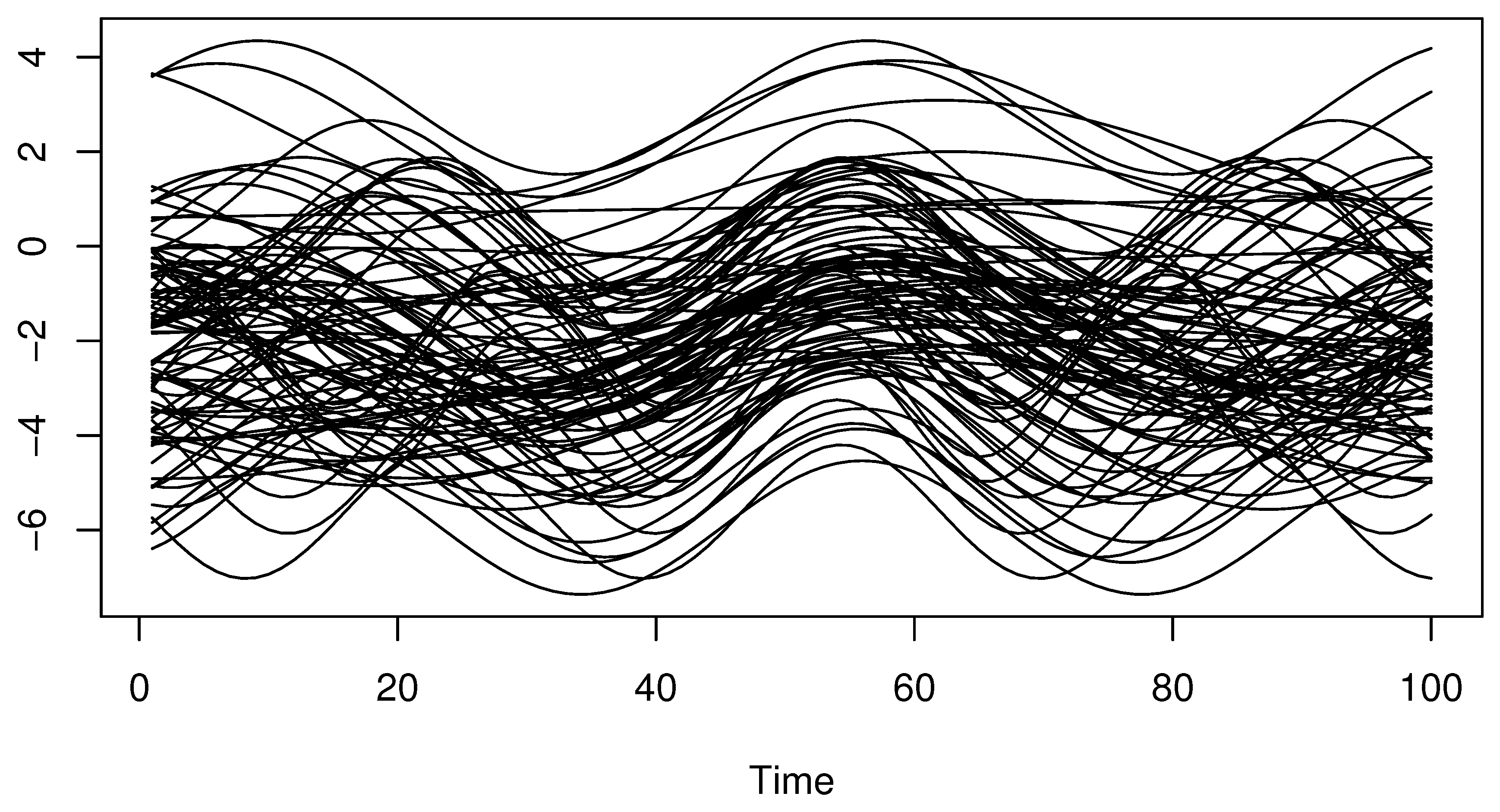
We generate a sequence of functional exploratory variables from

$$X\left(t\right)=sin\left(W_{1}t\right)+cos\left(W_{1}t\right)+2W_2,$$

(9)

where $W_1$ follows $N(1,1)$ and $W_2$ follows $N(-1,1)$. Such a sample of curves ${\mathcal{X}}_i$s is discretized in 100 equi-spaced grids in $(-2\pi ,2\pi )$. The functional curves are presented in Figure 1.

Step 2.

We generate the output variable Y using a functional regression model

$$Y=\frac{1}{2\pi }{\int }_{-2\pi }^{2\pi }\frac{X^2\left(t\right)}{1+X^2\left(t\right)}dt+ϵ,$$

(10)

where $ϵ$ is independent of X and has a Laplace distribution. This sampling algorithm shows that the law of $Y\mid X$ is defined by shifting the distribution of $ϵ$.

Next, to incorporate the theoretical part of this work, we pay attention in this comparative study to analyzing the behavior of the estimator using various missing levels. Specifically, we compare the resistance of the estimators ${\widehat{Q}}_{\alpha }$, ${\tilde{Q}}_{\alpha }$, and ${\overline{Q}}_{\alpha }$ using different missing rates. Furthermore, the missing phenomena are modeled as

$$P\left(X\right)=\mathtt{expit}\left(\frac{2\lambda }{\pi }{\int }_{-2\pi }^{2\pi }\frac{1}{1+X^2\left(t\right)}dt\right),$$

where $\mathtt{expit}\left(u\right)=e^u/(1+e^u)$. This consideration allows us to control the missing rate through the parameter $\lambda$. Typically, we examine three levels of censoring levels, which are strong, medium, and weak, which correspond to $\lambda =0.05$, $\lambda =0.5$, and $\lambda =5$, respectively. Empirically, the missing level is evaluated by

$$\overline{\delta }=\frac{1}{n}\sum _{i=1}^n{\delta }_i.$$

For the above values of $\lambda$, we observe that there are 5% missed observations when $\lambda =5$; 30% missed observations for $\lambda =0.5$; and more than 57% missing observations when $\lambda =0.05$.

Step 3.

We calculate the three estimators ${\widehat{Q}}_{\alpha }$, ${\tilde{Q}}_{\alpha }$, and ${\overline{Q}}_{\alpha }$. For the practical computation of these estimators, we consider a kernel $Ke$ as a quadratic kernel

$$Ke\left(t\right)=\frac{3}{2}(1-t^2)1\mathrm{I}[0,1)$$

and we choose the locating functions δ and ℓ defined by

$$\ell (v,x^{\prime })={\left(\int {({\mathcal{X}}^{\left(2\right)}\left(t\right)-{\mathcal{X}}^{\prime \left(2\right)}\left(t\right))}^{2}dt\right)}^{1/2}\mathrm{and} \ell (v,x^{\prime })=\int \theta \left(t\right)({\mathcal{X}}^{\left(2\right)}\left(t\right)-{\mathcal{X}}^{\prime \left(2\right)}\left(t\right))dt$$

where ${\mathcal{X}}^{\left(i\right)}$ denotes the ith derivative of x, and $\theta$ denotes the eigenfunction associated with the greatest eigenvalue of the covariance matrix

$${\displaystyle \frac{1}{n}\sum _{j=1}^n{(X_j^{\left(i\right)}-\overline{X^{\left(i\right)}})}^t(X_j^{\left(i\right)}-\overline{X^{\left(i\right)}}).}$$

The estimators are calculated using the straightforward modification of the routine code cond.quantile in the R package fda.usc. To highlight the flexibility of our estimation approach, we compare two selection procedures to select the optimal k and the optimal h. The first one is based on

$$\begin{array}{c}{\displaystyle MSE=\frac{1}{n}\sum _{i=1}^n{\Xi }_{\alpha }\left({\mathcal{Y}}_i-{\ddot{T}}_{\alpha }\left({\mathcal{X}}_i\right)\right)\mathrm{rule}\left(1\right)}\end{array}$$

where ${\ddot{T}}_{\alpha }$ refers to the leave-one-out curve estimator of ${\widehat{Q}}_{\alpha }$, ${\tilde{Q}}_{\alpha }$, and ${\overline{Q}}_{\alpha }$. Meanwhile, the second one is based on the mean square error cross-validation rule defined by

$$\begin{array}{c}{\displaystyle MSE=\frac{1}{n}\sum _{i=1}^n{\left({\mathcal{Y}}_i-{\ddot{T}}_{0.5}\left({\mathcal{X}}_i\right)\right)}^2\mathrm{rule}\left(2\right).}\end{array}$$

This rule is optimized over k in $\{5,10,15,\dots ,60\}$ and over h, the q-quantile of the vector distance between the curves ($q=0.1,0.2,0.3,0.4,0.5$).

The finite sample performance of the above estimators is evaluated through the MAE error, expressed by

$${\displaystyle MAE=\frac{1}{n}\sum _{i=1}^n\left|Q_{\alpha }\left({\mathcal{X}}_i\right)-{\ddot{T}}_{\alpha }\left({\mathcal{X}}_i\right)\right|.}$$

(11)

We report the MAE errors of the three estimators in

Table 1. Comparison of the MAE between different quantile estimations.

Estimator	Quartile	Rule	n	$\mathit{\lambda }=5$	$\mathit{\lambda }=0.5$	$\mathit{\lambda }=0.05$
Estimator ${\tilde{Q}}_{\alpha }$	Q1	1	50	0.2358	0.3997	0.4672
		2	50	0.2067	0.2676	0.3879
		1	250	0.1407	0.2340	0.3717
		2	250	0.1835	0.1980	0.2140
Estimator ${\widehat{Q}}_{\alpha }$	Q1	1	50	0.3672	0.4426	1.0578
		2	50	0.7697	1.1725	1.7811
		1	250	0.3086	0.3508	0.682
		2	250	0.4162	0.5117	0.8106
Estimator ${\overline{Q}}_{\alpha }$	Q1	1	50	1.3672	1.6426	1.0578
		2	50	1.7697	1.9725	2.7811
		1	250	0.9086	1.3508	1.4282
		2	250	1.0462	1.5117	1.9106
Estimator ${\tilde{Q}}_{\alpha }$	Q2	1	50	0.1840	0.2253	0.4102
		2	50	0.2005	0.2339	0.3650
		1	250	0.0912	0.1873	0.1494
		2	250	0.1101	0.1991	0.1616
Estimator ${\widehat{Q}}_{\alpha }$	Q2	1	50	0.0657	0.1650	0.2107
		2	50	0.0984	0.1922	0.188
		1	250	0.0677	0.0971	0.1478
		2	250	0.0327	0.0303	0.0643
Estimator ${\overline{Q}}_{\alpha }$	Q2	1	50	0.6967	0.9824	1.0788
		2	50	0.4176	0.4521	0.6588
		1	250	0.2952	0.3880	0.4950
		2	250	0.2965	0.3718	0.4301
Estimator ${\tilde{Q}}_{\alpha }$	Q3	1	50	1.851	2.5103	3.2202
		2	50	1.2035	3.3339	3.5650
		1	250	1.7182	1.4723	2.5494
		2	250	1.3111	1.3991	2.18616
Estimator ${\widehat{Q}}_{\alpha }$	Q3	1	50	0.9257	1.0350	1.1317
		2	50	1.0804	1.1232	1.188
		1	250	0.7017	0.9751	1.0278
		2	250	0.6127	0.8303	0.9613
Estimator ${\overline{Q}}_{\alpha }$	Q3	1	50	2.6907	2.7824	4.8898
		2	50	1.8176	1.8251	1.9688
		1	250	1.1479	1.1780	1.18950
		2	250	1.0985	2.0898	2.1201

. This table summarizes the results for different missing levels, different sample sizes, different selectors, and three quartiles, $Q1$, $Q2$, and $Q3$.

Unsurprisingly, KNN–LLA appears to be preferred over the other estimators. In particular, for various situations, the MAE of KNN–LLA is between $(0.06,1.12)$ and $(0.09,3.22)$ for the fixed-bandwidth LLA. Both estimators are significantly more efficient than the estimator ${\overline{Q}}_{\alpha }$. It produces an MSE ranging within $(0.29,4.88)$. Such a result shows the superiority of the LLA over the local constant method that is given in the statistical literature.

4.2. A Real Data Application

In this section, we illustrate the KNN–LLA of the quantile with regressor via a real data example. More precisely, we use the quantile with regressor to predict the riboflavin quantity in yogurt, using infrared curves. The latter is one of the B vitamins, which are crucial to yogurt’s quality. This vitamin is indispensable for the metabolism of protein, carbohydrates, and fats. It is one of the most important coenzymes necessary for antibody production, energy metabolism, cell respiration, growth, and development. The riboflavin prediction problem has been studied in many works in the past (see [36] for some algorithms). However, the novelty of the present work is the implementation of the functional KNN–LLA model in this forecasting problem. It is well documented that nonparametric tools are more widely adopted in this functional context. For this illustration, we employ 115 functions ${\mathcal{X}}_i\left(t\right)$, which represent light absorption at 120 waves. The wavelengths are selected to be between 270 and 550 nm. Such data are available at http://www.models.life.ku.dk/Yogurt (accessed on 31 December 2023). The functional data are plotted in Figure 2.

Furthermore, the output variable ${\mathcal{Y}}_i$ is the quantity of riboflavin. We have 115 observations of ${({\mathcal{X}}_i,{\mathcal{Y}}_i)}_{i=1,\dots 115}.$ We remove some observations from these data, and we compare two different strategies to handle the missing phenomenon. The first one is based on the ideas developed in the theoretical part of this work, where ${\mathcal{Y}}_i$ is predicted by ${\widehat{Q}}_{\alpha }\left({\mathcal{X}}_i\right)$. In the second strategy, we replace the missed observations ${\mathcal{Y}}_{i_0}$ with

$$\overline{{\mathcal{Y}}_{i_0}}=\frac{1}{k}\sum _{i=1}^k{\mathcal{Y}}_{i^{i_0}},$$

where $\left({\mathcal{Y}}_{i_0}\right)i=1,\dots k$ are the k observed response variables corresponding to the KNN explanatory observations at $X_{i_0}$. Furthermore, we use the same kernel and keep the same selectors to choose the smoothing parameter. However, the smoothed property of the spectrometry curves is dependent on the choice of the metric d, as well as the locating function $\delta$ and ℓ. From Figure 2, we see that the curves have a discontinuous form. Thus, the PCA metric is more suitable for this situation. In this sense, we proceed with $d=\delta =\ell$. Finally, for this comparative study, we split the data many times (exactly 70 times), in a random manner, into subsets (90% learning sample and 10% testing sample) and we compute the

$$\begin{array}{c}{\displaystyle MSE=\frac{1}{n}\sum _{i=1}^n{\left({\mathcal{Y}}_i-{\widehat{Q}}_{0.5}\left({\mathcal{X}}_i\right)\right)}^2}\end{array}$$

(12)

for both strategies. In the following figures, we give the boxplots for two cases: a moderate missing case (only 5% of observations are removed) and a strong missing case (45% of observations are removed).

Clearly, strategy 1 has significant advantages over strategy 2 (see Figure 3 and Figure 4). This conclusion reflects the statement made by [23]. The latter stated that the best way to handle the missing phenomenon is to ignore the missed observations. Indeed, the second strategy is based on double estimations, which can induce additional errors. Finally, we point out that the KNN estimation method is very easy to compute and fast to execute.

In the second illustration, we compare quantile regression to classical regression as estimated via the KNN–LLA approach in the functional MAR case using the same ideas. In this sense, the KNN–LLA estimator $\widehat{R\left(x\right)}$ of the classical regression $R\left(x\right)=E\left[Y\right|X=x]$ is

$$\begin{array}{cc}\hfill (\widehat{a},\widehat{b})={\displaystyle \underset{(a,b)\in {\mathbb{R}}^2}{min}}{\displaystyle \sum _{i=1}^n}{(Y_i-A-B\ell ({\mathcal{X}}_i,x))}^{2}Ke\left(h_k^{-1}\kappa (v,{\mathcal{X}}_i)\right),& \widehat{R\left(x\right)}=\widehat{a}.\end{array}$$

(13)

In particular, we compare it to median regression, which corresponds to $\widehat{Q_{0.5}\left(x\right)}$. We follow the same algorithm as in the first part, where strategy 1 is employed to model the missing observations. We use the same kernel, the same locating functions, and the same selector for the optimal number of neighborhoods. Now, in order to highlight the importance of median regression over classical regression, we compare their resistance to the outlier response data. To do this, we randomly multiply some observations by a varied constant C and we compare the absolute mean error

$$\begin{array}{c}{\displaystyle MA{E}_{q}uantile=\frac{1}{n}\sum _{i=1}^n\left|{\mathcal{Y}}_i-{\widehat{Q}}_{0.5}\left({\mathcal{X}}_i\right)\right|}\end{array}$$

(14)

and

$$\begin{array}{c}{\displaystyle MA{E}_{R}egression=\frac{1}{n}\sum _{i=1}^n\left|{\mathcal{Y}}_i-\widehat{R}\left({\mathcal{X}}_i\right)\right|.}\end{array}$$

(15)

We obtain the following result.

The result of

Table 2. Comparison of the resistance to outliers between conditional median and classical regression.

Constant C	Median Regression	Classical Regression
C = 1	1.37	1.72
C = 2	1.66	4.79
C = 5	2.24	10.17
C = 10	4.18	45.24

confirms the superiority of quantile regression over classical regression, namely through its robustness property. It is clear that median regression is more robust than classical regression. In this sense, the variability of the MAE error with respect to the multiplicative constant C is more important in classical regression than in the median case.

5. Conclusions

This contribution focuses on the free distribution approximation of the quantile function. Based on the KNN–LLA approach, we construct a new estimator. Its asymptotic property is proven under a missing structure. The employment of this approach is checked through artificial data. This analysis highlights the theoretical component, where we conclude that the performance of the estimator is affected by the level of the missing aspects. One of the main features of the KNN–LLA approach is the possibility to derive the consistency of the estimator when the smoothing parameter is also a random variable. Such a statement allows us to diversify the selection procedure for the best number of neighborhoods. The present work also provides a number of important directions for the future. The first is the establishment of the limit law of the KNN–LLA estimator under the independence or dependence case. Generalizing the present results to some functional time series or spatial curve data constitutes an interesting direction too. The latter would permit us to enhance the practical relevance of the KNN–LLA estimator in quantile regression and increase the applicability of this model to more important, real-world problems, such as economic forecasting, climate modeling, or medical statistics. In addition to these future directions, the treatment of alternative functional models and/or other smoothing methods could be considered, such as the single index model, the polynomial LLA, or the recursive algorithm, among others.

References

1. Samanta, M. Nonparametric estimation of conditional quantiles. Statist. Probab. Lett. 1989, 7, 407–412. [Google Scholar] [CrossRef]
2. Gannoun, A.; Saracco, J.; Yu, K. Nonparametric prediction by conditional median and quantiles. J. Statist. Plann. Inference 2003, 117, 207–223. [Google Scholar] [CrossRef]
3. Zhou, Y.; Liang, H. Asymptotic normality for L1 norm Kernel estimator of conditional median under K-mixing dependence. J. Multivar. Anal. 2000, 73, 136–154. [Google Scholar] [CrossRef]
4. Cardot, H.; Crambes, C.; Sarda, P. Estimation spline de quantiles conditionnels pour variables explicatives fonctionnelles. C. R. Math. Acad. Sci. Paris 2004, 339, 141–144. [Google Scholar] [CrossRef]
5. Ferraty, F.; Laksaci, A.; Vieu, P. Estimating some characteristics of the conditional distribution in nonparametric functional models. Stat. Inference Stoch. Process. 2006, 9, 47–76. [Google Scholar] [CrossRef]
6. Dabo-Niang, S.; Laksaci, A. Estimation non paramétrique de mode conditionnel pour variable explicative fonctionnelle. C. R. Math. Acad. Sci. Paris 2007, 344, 49–52. [Google Scholar] [CrossRef]
7. He, F.Y.; Cheng, Y.B.; Tong, T.J. Nonparametric estimation of extreme conditional quantiles with functional covariate. Acta Math. Sin. (Engl. Ser.) 2018, 34, 1589–1610. [Google Scholar] [CrossRef]
8. Laksaci, A.; Lemdani, M.; Ould Saïd, E. A generalized l1-approach for a Kernel estimator of conditional quantile with functional regressors: Consistency and asymptotic normality. Stat. Probab. Lett. 2009, 79, 1065–1073. [Google Scholar] [CrossRef]
9. Laksaci, A.; Maref, F. Estimation non paramétrique de quantiles conditionnels pour des variables fonctionnelles spatialement dépendantes. Comptes Rendus Math. 2009, 347, 1075–1080. [Google Scholar] [CrossRef]
10. Al-Awadhi, F.A.; Kaid, Z.; Laksaci, A.; Ouassou, I.; Rachdi, M. Functional data analysis: Local linear estimation of the L 1-conditional quantiles. Stat. Methods Appl. 2019, 28, 217–240. [Google Scholar] [CrossRef]
11. Baìllo, A.; Grané, A. Local linear regression for functional predictor and scalar response. J. Multivar. Anal. 2009, 100, 102–111. [Google Scholar] [CrossRef]
12. Berlinet, A.; Elamine, A.; Mas, A. Local linear regression for functional data. Ann. Inst. Stat. Math. 2011, 63, 1047–1075. [Google Scholar] [CrossRef]
13. Barrientos, J.; Ferraty, F.; Vieu, P. Locally Modelled Regression and Functional Data. J. Nonparametr. Statist. 2010, 22, 617–632. [Google Scholar] [CrossRef]
14. Demongeot, J.; Laksaci, A.; Madani, F.; Rachdi, M. Functional data: Local linear estimation of the conditional density and its application. Statistics 2013, 47, 26–44. [Google Scholar] [CrossRef]
15. Demongeot, J.; Laksaci, A.; Rachdi, M.; Rahmani, S. On the local linear modelization of the conditional distribution for functional data. Sankhya A 2014, 76, 328–355. [Google Scholar] [CrossRef]
16. Chouaf, A.; Laksaci, A. On the functional local linear estimate for spatial regression. Stat. Risk Model. 2012, 29, 189–214. [Google Scholar] [CrossRef]
17. Xiong, X.; Zhou, P.; Ailian, C. Asymptotic normality of the local linear estimation of the conditional density for functional time-series data. Commun. -Stat.-Theory Methods. 2018, 47, 3418–3440. [Google Scholar] [CrossRef]
18. Demongeot, J.; Naceri, A.; Laksaci, A.; Rachdi, M. Local linear regression modelization when all variables are curves. Stat. Probab. Lett. 2017, 121, 37–44. [Google Scholar] [CrossRef]
19. Chahad, A.; Ait-Hennani, L.; Laksaci, A. Functional local linear estimate for functional relative-error regression. J. Stat. Theory Pract. 2017, 11, 771–789. [Google Scholar] [CrossRef]
20. Rubin, D.B. Inference and missing data. Biometrika 1976, 63, 581–592. [Google Scholar] [CrossRef]
21. Josse, J.; Reiter, J.P. Introduction to the special section on missing data. Stat. Sci. 2018, 33, 139–141. [Google Scholar] [CrossRef]
22. Little, R.; Rublin, D. Statistical Analysis with Missing Data, 2nd ed.; John Wiley: New York, NY, USA, 2002. [Google Scholar]
23. Efromovich, S. Nonparametric Regression with Predictors Missing at Random. J. Am. Stat. Assoc. 2011, 106, 306–319. [Google Scholar] [CrossRef]
24. Ferraty, F.; Sued, F.; Vieu, P. Mean estimation with data missing at random for functional covariables. Statistics 2013, 47, 688–706. [Google Scholar] [CrossRef]
25. Ling, N.; Liang, L.; Vieu, P. Nonparametric regression estimation for functional stationary ergodic data with missing at random. J. Statist. Plann. Inference 2015, 162, 75–87. [Google Scholar] [CrossRef]
26. Ling, N.; Liu, Y.; Vieu, P. Conditional mode estimation for functional stationary ergodic data with responses missing at random. Statistics 2016, 50, 991–1013. [Google Scholar] [CrossRef]
27. Bachir Bouiadjra, H. Conditional hazard function estimate for functional data with missing at random. Int. J. Stat. Econ. 2017, 18, 45–58. [Google Scholar]
28. Almanjahie, I.M.; Mesfer, W.; Laksaci, A. The K nearest neighbors local linear estimator of functional conditional density when there are missing data. Hacet. J. Math. Stat. 2022, 51, 914–931. [Google Scholar] [CrossRef]
29. Yu, K.; Jones, M. Local linear quantile regression. J. Am. Stat. Assoc. 1998, 93, 228–237. [Google Scholar] [CrossRef]
30. Hallin, M.; Lu, Z.; Yu, K. Local linear spatial quantile regression. Bernoulli 2009, 15, 659–686. [Google Scholar] [CrossRef]
31. Bhattacharya, P.K.; Gangopadhyay, A.K. Kernel and nearest-neighbor estimation of a conditional quantile. Ann. Stat. 1990, 18, 1400–1415. [Google Scholar] [CrossRef]
32. Ma, X.; He, X.; Shi, X. A variant of K nearest neighbor quantile regression. J. Appl. Stat. 2016, 43, 526–537. [Google Scholar] [CrossRef]
33. Cheng, P.E.; Chu, C.K. Kernel estimation of distribution functions and quantiles with missing data. Stat. Sin. 1996, 6, 63–78. [Google Scholar]
34. Xu, D.; Du, J. Nonparametric quantile regression estimation for functional data with responses missing at random. Metrika 2020, 83, 977–990. [Google Scholar] [CrossRef]
35. Kara-Zaitri, L.; Laksaci, A.; Rachdi, M.; Vieu, P. Data-driven kNN estimation for various problems involving functional data. J. Multivar. Anal. 2017, 153, 176–188. [Google Scholar] [CrossRef]
36. Becker, E.M.; Christensen, J.; Frederiksen, C.S.; Haugaard, V.K. Front-face fluorescence spectroscopy and chemometrics in analysis of yogurt: Rapid analysis of riboflavin. J. Dairy Sci. 2003, 86, 2508–2515. [Google Scholar] [CrossRef]
Figure 1. A sample of functional regressors.
Axioms 13 00444 g001
Figure 2. The spectral curves.
Axioms 13 00444 g002
Figure 3. Comparison of the MSE between the two strategies in the moderate missing case.
Axioms 13 00444 g003
Figure 4. Comparison of the MSE between the two strategies in the strong missing case.
Axioms 13 00444 g004