Abstract
This mathematical model delves into the dynamics of the immune system during Chronic Myeloid Leukemia (CML) therapy with imatinib. The focus lies in elucidating the allergic reactions induced by imatinib, specifically its impact on T helper (Th) cells and Treg cells. The model integrates cellular interactions, drug pharmacokinetics, and immune responses to unveil the mechanisms underlying the dominance of Th2 over Th1 and Treg cells, leading to allergic manifestations. Through a system of coupled delay differential equations, the interplay between healthy and leukemic cells, the influence of imatinib on T cell dynamics, and the emergence of allergic reactions during CML therapy are explored.
Keywords:
chronic myeloid leukemia; imatinib therapy; mathematical modeling; immune system dynamics; T cell subset modulation; allergic reactions; pharmacokinetics; cellular interactions; Th1; Th2; Treg cells; stem-like; mature cell populations; time delays; differential equations; pharmacodynamics MSC:
34K20; 92C50; 92D25
1. Introduction
Chronic Myeloid Leukemia (CML) is a hematological malignancy characterized by the presence of the BCR-ABL fusion gene, which produces an abnormal tyrosine kinase protein. This protein is responsible for the uncontrolled proliferation of leukemic cells. The introduction of imatinib, a targeted tyrosine kinase inhibitor, has revolutionized the treatment of CML by specifically inhibiting this abnormal protein, leading to significant improvements in patient outcomes.
However, despite its efficacy, imatinib therapy is associated with a range of immune-related side-effects, including allergic reactions. These adverse effects are believed to result from the drug’s impact on various components of the immune system, particularly T helper (Th) cells and regulatory T cells (Tregs). Understanding the underlying mechanisms of these immune responses is crucial for improving the management of CML patients undergoing imatinib therapy.
The significance of this study lies in its potential to bridge the gap in our understanding of the immune dynamics during imatinib treatment. By developing a comprehensive mathematical model, we aim to elucidate the interactions between imatinib, leukemic cells, and the immune system. This model incorporates cellular interactions, drug pharmacokinetics, and immune responses, providing a detailed framework to study the emergence of allergic reactions and other immune-related side-effects.
Previous studies, in which delay differential equations (DDEs) are used to model the CML-immune dynamics, have primarily focused on how to model the evolution of healthy and leukemic cells and the direct effects of treatment on leukemic cells (see [1,2,3,4,5,6,7,8,9,10,11,12,13]). However, these studies offer limited exploration of its broader impact on the immune system. To address this, we added to the model new equations that account for allergic reactions, relying on [14,15,16]. The mathematical model introduced in this paper, bridges this gap by integrating the modulation of Th cell subsets and the resulting shift in immune balance. Specifically, we investigate the dominance of Th2 cells over Th1 and Treg cells, which is hypothesized to contribute to the allergic manifestations observed during therapy.
By employing a system of coupled delay differential equations, our model captures the temporal dynamics of cellular processes and drug interactions. This approach allows us to simulate the progression of CML and the corresponding immune responses over time, providing insights into the mechanisms driving the observed clinical outcomes.
2. The Mathematical Model
The mathematical model aims to capture the complexities of the immune response during CML therapy, with a specific focus on the alteration of T cell subsets, induced by imatinib. The model encompasses various cell populations, including stem-like healthy and leukemic cells, mature cells, and distinct T cell subsets (Th1, Th2, and Treg). Additionally, it incorporates the pharmacokinetics of imatinib, shedding light on its absorption and distribution within the body. Furthermore, the model explores the differentiation of naive T cells into effector states, considering positive growth and suppressive signals.
In what follows, we first discuss the biological aspects and assumptions and the mathematical implications of the said assumptions and then we introduce the model and describe its equations.
We integrate the modulation of naive APC cells by imatinib and leukemic cells. This integration suggests a potential shift in the balance of Th cell subsets, with a dominance of Th2 cells over Th1 and Treg cells. Understanding this shift is critical for elucidating the allergic reactions triggered during CML therapy. As shown by Segel [17], Th2 cells stimulate the production of IgE, while Th1 cells promote the production of IgG (refer to Behn [14]). Thus, a transition from a Th2-dominated memory state to a Th1-dominated memory state indicates successful chemotherapy without allergic reactions.
The model considers both healthy and leukemic cell populations, possessing self-renewal capabilities, denoted as and , respectively. These are referred to as stem-like cells, assumed to undergo a brief period of quiescence categorized as short-term hematopoietic stem cells (ST-HSC).
Two additional populations, and , represent mature healthy and leukemia leukocytes, respectively. The immune system is characterized by , representing naive APCs, mature APCs, naive CD4+, Th1, Th2, Th3, Tregs, naive CD8+, and CD8+ cytotoxic T cells actively targeting leukemic cells. The competition between healthy and leukemic blood cell populations for resources is considered in the feedback laws governing self-renewal and differentiation.
Thus, the rate of self-renewal is
(h for healthy and l for leukemia) with the maximal rate of self-renewal and half of the maximal value.
The rate of differentiation is
Now, is the maximal rate of differentiation and is half of the maximal value.
It is assumed that a fraction , where , of short-term hematopoietic stem cells (ST-HSC) is prone to asymmetric division: one daughter cell undergoes differentiation, while the other re-enters the stem cell compartment. Another fraction, , where , is inclined to differentiate symmetrically, yielding two cells that mature, while the remaining fraction , where , is predisposed to self-renewal, resulting in two stem-like cells after mitosis.
Moreover, the model includes feedback functions regulating the immune system, reflecting the modulation of naive APC cells by imatinib and the resulting shift in the balance of Th-cell subsets. Recognizing that active CD4+ T helper cells secrete positive growth/suppressive signals at varying rates, we introduce T-helper-dependent feedback functions. These functions model positive growth signals for T cells’ self-development (autocrine loop) and stimulation of further division in T cytotoxic cells. Additionally, they account for suppressive signals resulting from the regulatory process. Here, the inhibitory effects of imatinib on Treg development are considered. Leukemic cells also exert an influence on the evolution of CD8+ cytotoxic T cells, suppressing the effect of the immune system.
The following feedback functions regulate the evolution of the immune system and its interaction with leukemic cells ([3,7]):
- —it balances the effect of the immune system on the leukemic cells and it depends on the total number of leukemic cells (naive and mature);
- —it controls the activation of APCs depending on the number of mature leukemic cells;
- —it regulates the immune response through the number of mature leukemic cells;
- —it regulates the population CD8+ mature cells through T-reg cells.
The therapeutic strategy targeting the BCR-ABL gene is presumed to impact the apoptosis of leukemia cells and the proliferation rates of both healthy and leukemia cells. Its effect is considered constant over time, reflecting a period where, following an initial transitory stage, the cellular impact stabilizes. Imatinib plays a crucial role in modulating the maturation and proper functioning of Antigen-Presenting Cells (APCs) and, consequently, T cells within the immune system.
Treatment effects are incorporated into the model through the factor in terms controlling leukemic stem-like cell multiplication, and factors , , and in the equation of the immune system’s cells. To determine the relationship between , and and the drug concentration in the plasmatic compartment , we rely on experimental data. Details on the choice of functions governing treatment influence on different cell lines can be found in [6]. Thus, influences the leukemic stem cells. influences the APC. The activation of T cells is controlled by . Finally, reduces the self-stimulation of T-helper cells.
As shown by Segel [17], Th2 cells stimulate the production of IgE, while Th1 cells promote the production of IgG (refer to Behn [14]). Consequently, a transition from a Th2-dominated memory state to a Th1-dominated memory state indicates successful chemotherapy without the occurrence of allergic reactions.
Among various regulatory T cells, the induced regulatory T cells () are crucial in the context of allergic reactions (Behn [14]). These cells release cytokines like IL-10 and TGF-, capable of suppressing both Th1 and Th2 immune responses. Their differentiation from naive T cells follows a similar process as observed in other subsets (see Behn [14]).
The procedure known as drug desensitization assists patients in tolerating medications that previously triggered hypersensitive reactions. According to [18], by employing a gradual desensitization approach, all patients successfully tolerated a daily dose of 400 mg of imatinib, and the dosage of prednisolone was systematically reduced. The proportions of imatinib-induced CD4+CD25+CD134+ T cells declined from an initial mean (SD) of 11.3% (6.5%) and 13.4% (7.3%) to 3.2% (0.7%) and 3.0% (1.1%) following effective desensitization. This was observed when stimulating peripheral blood mononuclear cells with 1 and 2 mM of imatinib, respectively.
Time delays are incorporated to reflect the duration of cellular processes, introducing temporal dynamics to the model.
In order to model the CML-immune dynamics under therapy, we use a system of delayed differential equations (DDEs). We base the model on former work ([3,8,15]) and some classic models from the literature (see ([1,2,14,19])). We offer more details on the source of inspiration in the model description.
The complete model consists of the following equations:
The previous system can be written as
In what follows, details are given on the form of the equations as well as on the occurring parameters.
Equation (1) represents the state variable , the concentration of stem-like healthy cells, the rate of self-renewal , and the rate of differentiation with ; where cell competition (healthy vs. leukemic) was taken into account, and (see [1,2]). These first four equations were introduced in [8] (see also [3]).
Equation (2) represents the concentration of mature healthy cells .
Equation (3) represents the concentration of stem-like leukemic cells .
Equation (4) represents the concentration of mature leukemic cells .
The last terms in Equations (3) and (4) stand for the mortality of the leukemic cells due to the interaction with the cytotoxic T cells (for a similar representation of this process, see [19]).
In Equation (5), represents the concentration of naive antigen-presenting cells (APCs). Here, is a constant supply of naive APCs even in the absence of any disease, and is the apoptosis rate of naive APCs. The third term accounts for the rate of APC activation by the antigen induced during therapy with imatinib. The last term represents the activation of naive APCs due to the encounter with leukemia cells. The treatment is involved in these activations through .
In Equation (6), represents the concentration of mature APCs activated by the antigen induced by the drug. Here, denotes the apoptosis rate of mature APCs. The second term in the equation accounts for the influx of mature APCs from the naive pool due to activation by the antigen during therapy with imatinib.
Equation (7) represents the dynamics of APC cells activated by leukemic cells, . The first term denotes natural degradation, and the second term refers to the activation of APC cells by leukemic cells.
In Equation (8), represents the concentration of naive CD4+ T cells, which are produced at a constant rate . The second term represents the degradation of these naive cells. The last three terms stand for the differentiation of naive cells into Th1, Th2, and Treg, respectively, under the action of APCs [14].
In Equation (9), represents the variation in concentration of Th1 cells, which is proportional to the concentration of naive cells timed with the concentration of APCs stimulated by the allergen with a delay . The first term represents the degradation of Th1 cells, and the second term represents the differentiation of naive cells into Th1, diminished due to suppression by Treg and Th2 cells.
In Equation (10), represents the concentration of Th2, which is proportional to the concentration of naive cells timed with the concentration of APCs and the concentration of their respective cytokines. The first term represents the degradation of Th2 cells, and the second term represents the differentiation of naive cells into Th2, divided by the suppression of Treg and Th1 cells. Remark that the suppression is modeled by factors of the form , where x stands for the concentration of cytokines produced by the suppressing population [14].
In Equation (11), represents the concentration of Treg, which is proportional to the concentration of naive cells timed with the concentration of APCs. The first term represents the degradation of Treg cells, and the second term represents the differentiation of naive cells into Treg. In Equations (9)–(11), the parameter determines how many differentiated T cells arise from a single naive cell. p and account for differences in autocrine action between the three subsets. The suppression strength of Th1, Th2, and Treg is controlled by the parameters , in that order. The treatment effects are introduced in these equations through the factor that controls multiplication [20].
In Equation (12), represents the concentration of the population of naive CD8+ cells. The first term denotes the supply rate, the second term denotes natural degradation, and the last term represents the loss due to maturation under the action of APCs activated by leukemic cells.
In Equation (13), represents the concentration of mature CD8+ T cells. The first term represents the naive cells activated by APCs after m divisions, the second term represents the active CD8+ T cells that are suppressed by Tregs, the third term represents the suppression of the immune response by leukemia cells, and it is assumed that the level of down-regulation depends on the current leukemia population. This suppressive action is expressed by the presence of the mature population of leukemia cells in the denominator of the function . The last two terms represent the stimulation of cell divisions due to positive growth signals induced by IL-2 secreted by both CD4+ and CD8+ mature cells. The time delays and , where is the duration of the T cell division cycle, are supposed equal for naive and mature CD8+ cells.
In Equation (14), represents equations for imatinib pharmacokinetics following [21]. Here, stands for the amount of drug in the absorption compartment. is the absorption rate in the first compartment, and K, the dose of drug administered in a unit of time, is taken to be constant.
In Equation (15), represents the amount of drug in the plasmatic compartment. v is the total plasma clearance of the drug divided by the volume of distribution of the drug.
Let .
The delays for healthy and leukemia ST-HSC cells are and , representing the duration of the cell cycle independent of the type of division. and denote the time needed for differentiation into mature leukocytes for healthy and leukemia cells, respectively. The fifth delay, , is due to the time for propagation of the allergen from the central compartment to the peripheral compartment [22]. If T is the infusion time interval and is a pharmacokinetic parameter related to the transition between the central and peripheral compartments, one has, following [22], .
The delay is the time necessary for naive CD8+ cell maturation, and is the time necessary for divisions.
Define .
We refer to previous works [1,3,7] for parameter significance, interpretation, and justification.
The last two equations are decoupled from the rest of the system, so will be considered as an external parameter.
3. Positivity of Solutions
For the system (16), a Cauchy problem is defined by considering the initial data in :
First of all, the essential positivity of the solutions will be established.
Proposition 1.
Proof.
From Equations (1)–(4) and (13) one can observe that, due to the delayed terms, if, for some , one has for some , then and one cannot have negative values for . The same reasoning works for . Since
it follows that, once is proved to be positive for all , if . Then, result positive by the argument used at the beginning of the proof. Also, since
it follows that in the domain of existence. Similar formulae hold for so, first, results to be strictly positive and finally has the same property. □
4. Stability of Some Equilibria
4.1. The Equilibrium Point
The first equilibrium point to be considered is corresponding to the death of the patient.
In order to study the characteristic equation, one has to compute the matrices , the matrix of partial derivatives with respect to undelayed variables calculated in , , the matrix of partial derivatives with respect to delayed variables, and similarly, , , , , , .
The characteristic equation factorizes as
The characteristic equation becomes:
Stability conditions: To study the stability of the equations , , and , we apply the well-known criteria that can be found in [23,24].
Since , , , (see Appendix A), one has stability for all positive if:
4.2. The Equilibrium Point
Consider next that can be interpreted as a healthy state, with undetectable leukemia cells and no allergic reactions.
The nonzero terms in the matrices of partial derivatives calculated this time in are to be found in the Appendix A. The matrix
is block triangular, so its determinant factors as
with
where
According to the already cited criterion from [23,24], since , and , is stable if:
- The roots of have negative real parts.
We now study the roots of
with the aim of establishing when they have a negative real part (see also [25]).
Suppose that for , the Equation (23) is stable. Then, stability can be lost if, and only if, the roots of (23) cross the imaginary axis from left to right, as the delays vary. This can happen only if pure imaginary roots can appear, so consider the equation , . The Equation (23) becomes:
Now, we look for conditions under which has no real roots w. We will analyze the equation and see if there are any specific conditions on the coefficients and parameters that would prevent the existence of real roots.
To solve , express the exponential terms in trigonometric form:
Substituting these expressions back into , we obtain:
Separate the real and imaginary parts of and then square each of them, following the approach in [26].
Introduce the real and imaginary parts through , where is the real part and is the imaginary part. Then,
Condition 4 is verified if the following equation has no positive roots.
Concerning the stability for , one has
and (23) is stable for if, and only if, and .
4.3. Equilibrium Point
Another interesting equilibrium point is , which represents a successful cure but with the persistence of allergic reactions.
The nonzero terms in the matrices of partial derivatives calculated in are found in the Appendix A.
To study the stability of , remark that the matrix
is block triangular, so its determinant factors as
Remark that
with and defined in (19)–(22).
Also
with
Once again, since , is stable if:
- The roots of have negative real parts
- The roots of have negative real parts
The study of the roots of
is already performed for the study of the stability of .
The analysis of condition 5 parallels the approach taken from Theorem 1 in [26] that we briefly recall.
Consider the equation , where and are analytic functions in the right half-plane , , which satisfy the following conditions:
- and have no common imaginary zero.
- , for real y (the upper bar denotes complex conjugate).
- .
- There are at most a finite number of roots of in the right half-plane when .
- , for real y, has at most a finite number of real zeroes.
It is evident that the above conditions are verified in our setting.
Under these conditions, the following statements are true:
- (a)
- Suppose that the equation has no positive roots. Then, if is stable at , it remains stable for all , and if it is unstable at , it remains unstable for all .
- (b)
- Suppose that the equation has at least one positive root and that each positive root is simple. As increases, stability switches may occur. There exists a positive number such that the equation is unstable for all . As varies from 0 to , at most, a finite number of stability switches may occur.
In what follows, the condition for to have no positive roots will be studied. and are given in (25).
We need to evaluate , square them, and ensure that remains non-positive for all positive y. Thus, we need to analyze the expression:
After simplification, the condition for :
This condition ensures that either or for all positive y.
We can expand these expressions:
and
The first equation, , becomes:
To find the conditions such that the equation in y has no positive roots for the given complex equation, we need to analyze both the real and imaginary parts separately.
Real Part: The real part of the equation is:
For this quadratic equation, the condition to have no positive roots follows easily.
Imaginary Part: Set the imaginary part equal to zero:
Introduce . If there are no positive roots of the imaginary part.
The second equation, , becomes:
To find the conditions such that the equation in y has no positive roots for the given complex equation, we need to analyze both the real and imaginary parts separately.
Real Part: The real part of the equation is:
For this quadratic equation, the condition to have no positive roots follows easily.
Imaginary Part: Set the imaginary part equal to zero:
Let us denote the coefficient term as:
So, the equation becomes:
For the given cubic equation , there are no positive roots if .
For , . This will be a stable polynomial if, and only if, (the Routh–Hurwitz criterion).
4.4. Equilibrium Point
The next equilibrium point, , represents a successful cure without allergic reactions. The conditions for its existence are listed in the Appendix A, together with the expressions of its components.
The nonzero terms in the matrices of partial derivatives calculated in are provided in Appendix A.
The determinant of the matrix
factors as
Since in this case we also have , , , and ,
is stable if:
- The following equation has negative rootsi.e.,
- The roots ofhave negative real parts.
For condition 5, we write as follows:
and use the analysis conducted for .
5. Parameters Values, Numerical Calculations, and Simulations
The following parameters are taken mainly from [2,6,9,19], some of them being just estimated, especially for leukemia cells.
| The production rate of naive CD4+ cells [19] | 0.1 | |
| The strength of suppression rate of Th1 by Th2 [14] | 0.1 | |
| The strength of suppression of Th2 by Th1 [14] | 0.2 | |
| The strength of suppression rate by Treg [14] | 0.5 | |
| The differences in the autocrine action of the three subsets [14] | p | 0.05 |
| The differences in the autocrine action of the three subsets [14] | 0.1 | |
| The death rate of cells [27] | ||
| The death rate of cells [27] | ||
| The death rate of cells [27] | ||
| The proliferation rate of stimulated T cells [14] | 0.2 | |
| Time delay [22] | ||
| Initial number of immune cells [28] | = 0.1 in microliter |
5.1. Numerical Simulations and Computations for
A numerical study of the conditions of stability for the equilibrium point , based on the above-given parameters, gives the following:
Recall that, in order for equilibrium point to be stable, the first condition is that . The numerical computations show that this condition does not hold. We conclude that this equilibrium point is not stable.
This result can also be seen in the numerical simulations below in Figure 1. Although the simulations start with the same concentration for Th1 cells and Th2 cells, the evolution shows an immunological destabilization, as the concentration of Th2 cells is greater than that of Th1 cells.
| Parameter for the function for healthy cells | 1.77 | |
| Parameter for the function for leukemia cells | 2 | |
| Parameter for the function k for healthy cells | 0.1 | |
| Parameter for the function k for leukemia cells | 0.4 | |
| The maximum value of the function for leukemic cells | 0.5 | |
| The maximum value of the function for healthy cells | 0.5 | |
| The maximum value of the function k for leukemic cells | 36 | |
| The maximum value of the function k for healthy cells | 36 | |
| Parameter of the Hill function | 2 | |
| Parameter of the Hill function | 2 | |
| Parameter of the Hill function | 2 | |
| Parameter of the Hill function | 2 | |
| Loss of stem cells due to mortality and differentiation in other lines for leukemic cells | 0.04 | |
| Loss of stem cells due to mortality and differentiation in other lines for healthy cells [2] | 0.1 | |
| Rate of asymmetric division for leukemic cells | 0.1 | |
| Rate of asymmetric division for healthy cells | 0.7 | |
| Rate of symmetric division for leukemic cells | 0.7 | |
| Rate of symmetric division for healthy cells | 0.1 | |
| Loss of stem cells due to cytotoxic T cells | 0.03 | |
| Instant mortality of mature leukemic leukocytes | 1.2, 0.15 | |
| Instant mortality of mature normal leukocytes | 2.4 | |
| Amplification factor for leukemic leukocytes | 1400 | |
| Amplification factor for normal leukocytes [2] | 1200 | |
| Loss of mature leukocytes due to cytotoxic T cells | 0.6 | |
| Standard half-saturation in a Michaelis–Menten low | 6 | |
| Supply rate of immature APCs | 0.3/day | |
| Death/turnover rate of immature APCs | 0.03/day | |
| Coefficient of the activation due to imatinib | 1 | |
| Coefficient of the activation due to leukemia cells | 2 | |
| Death/turnover rate of mature APCs | 0.8/day | |
| Supply rate of naive T cells CD4+ phenotype | 2 | |
| Death/turnover rate of naive CD4+ cells | 0.03/day | |
| Death/turnover rate of effector CD4+ T helper cells | 0.23/day | |
| Supply rate of naive T cells CD8+ phenotype | 2 | |
| Death/turnover rate of naive CD8+ cells | 0.23/day | |
| Kinetic coefficient | 0.2 | |
| Coefficient of the positive growth signal [19] | 20 | |
| The number of antigen depending divisions | 6 | |
| Coefficient of inhibition due to Treg cells | 1 | |
| Coefficient of inhibition due to leukemic cells | 1.2 or 50 | |
| Number of divisions in minimal CD8+ developmental program | m | 4 |
| First-order absorbtion rate | 0.61 | |
| Dose of administrated drug | K | 0.2824 |
| Clearance rate | 0.0412 | |
| Duration of cell cycle for leukemia stem-like cells | 5.5 | |
| Duration of cell cycle for normal stem-like cells | 2.8 | |
| Duration of leukocyte cycle for leukemic cells | 5.4 | |
| Duration of leukocyte cycle for normal cells | 3.5 | |
| Duration of one CD4+ T cell division (bifurcation parameter) | 2.4 days | |
| Duration of one CD8+ T cell division | 1.4 days | |
| Duration of minimal developmental program, | 5.6 | |
| Duration of minimal developmental program, | 8.4 |
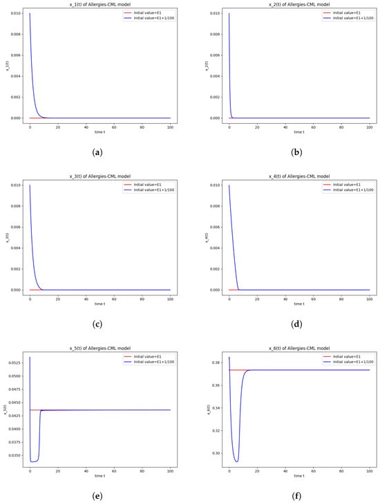
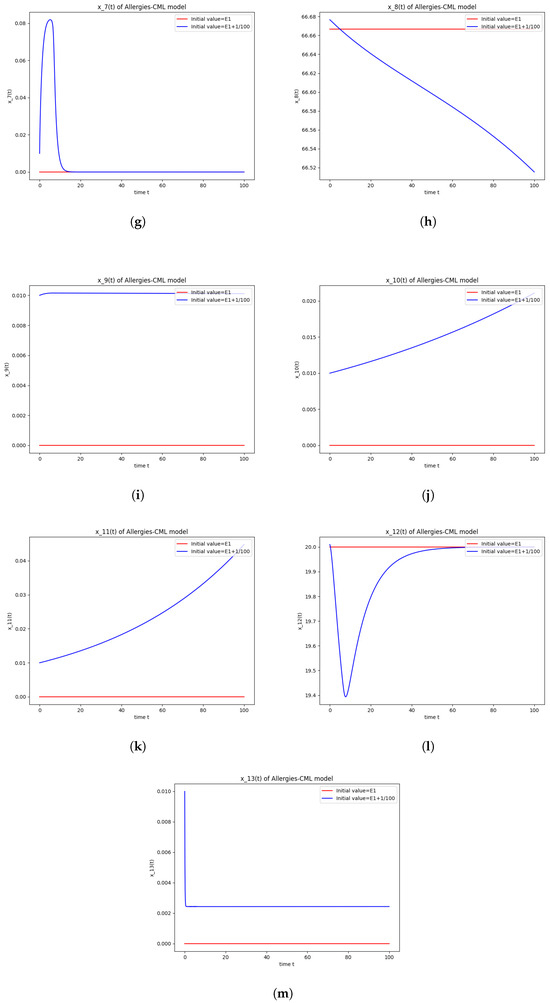
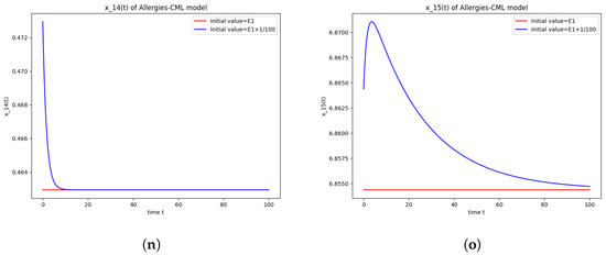
Figure 1.
Stability around the equilibrium point . (a) The concentration of stem-like healthy cells around . (b) The concentration of mature healthy cells around . (c) The concentration of stem-like leukemic cells around . (d) The concentration of mature leukemic cells around . (e) The concentration of naive APCs around . (f) The concentration of mature APCs activated by the drug around . (g) The concentration of mature APCs activated by the leukemic cells around . (h) The concentration of naive CD4+ T cells around . (i) The concentration of Th1 cells around . (j) The concentration of Th2 cells around . (k) The concentration of Treg cells around . (l) The concentration of naive CD8+ T cells around . (m) The concentration of mature CD8+ T cells around . (n) The amount of drug in the absorbtion compartment around . (o) The amount of drug in the plasmatic compartment around .
Furthermore, the simulations do not show a promising evolution of the patient’s condition, as both the healthy and the leukemic cells decrease to zero.
5.2. Numerical Simulations and Computations for
The equilibrium point is stable if:
- The roots of have negative real parts.
Numerical computations show that . Therefore, is not stable.
The numerical simulations performed around the equilibrium point indicate instability, validating the computations (Figure 2). It remains a healthy evolution, as the leukemic cells reduce to undetectable values and the healthy cells are attracted to a positive state. The balance of Th1–Th2 cells is towards Th2, so there are allergic reactions present.
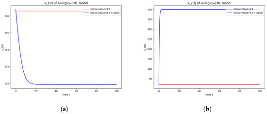
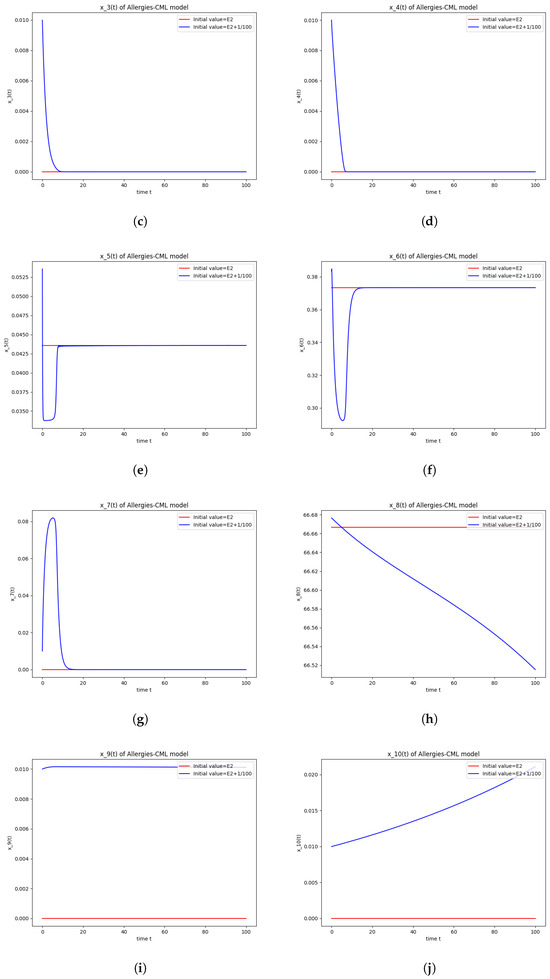
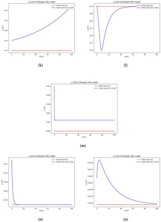
Figure 2.
Stability around the equilibrium point . (a) The concentration of stem-like healthy cells around . (b) The concentration of mature healthy cells around . (c) The concentration of stem-like leukemic cells around . (d) The concentration of mature leukemic cells around . (e) The concentration of naive APCs around . (f) The concentration of mature APCs activated by the drug around . (g) The concentration of mature APCs activated by the leukemic cells around . (h) The concentration of naive CD4+ T cells around . (i) The concentration of Th1 cells around . (j) The concentration of Th2 cells around . (k) The concentration of Treg cells around . (l) The concentration of naive CD8+ T cells around . (m) The concentration of mature CD8+ T cells around . (n) The amount of drug in the absorbtion compartment around . (o) The amount of drug in the plasmatic compartment around .
5.3. Numerical Simulations and Computations for
The equilibrium point is stable if the following parameter conditions hold:
- The roots of have negative real parts
- The roots of have negative real parts
According to the numerical calculations, . Therefore, is not stable.
The numerical simulations performed around the equilibrium point also seem to indicate instability (Figure 3). It has a positive evolution, as the leukemic cells die out and the concentration of Th1 cells shows rapid growth. The allergic reactions are still present due to the large concentration of Th2 cells, which greatly outnumber the Th1 cells.
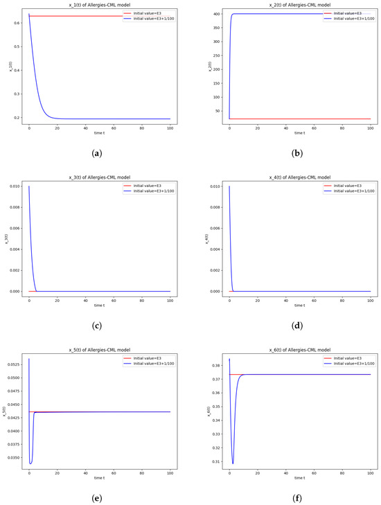
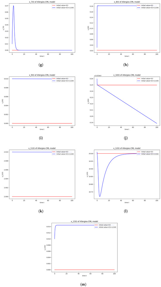
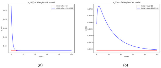
Figure 3.
Stability around the equilibrium point . (a) The concentration of stem-like healthy cells around . (b) The concentration of mature healthy cells around . (c) The concentration of stem-like leukemic cells around . (d) The concentration of mature leukemic cells around . (e) The concentration of naive APCs around . (f) The concentration of mature APCs activated by the drug around . (g) The concentration of mature APCs activated by the leukemic cells around . (h) The concentration of naive CD4+ T cells around . (i) The concentration of Th1 cells around . (j) The concentration of Th2 cells around . (k) The concentration of Treg cells around . (l) The concentration of naive CD8+ T cells around . (m) The concentration of mature CD8+ T cells around . (n) The amount of drug in the absorbtion compartment around . (o) The amount of drug in the plasmatic compartment around .
5.4. Numerical Simulations and Computations for
The equilibrium point is stable if:
- The following equation has negative rootsi.e.,
- The roots ofhave negative real parts.
The numerical computations have again found that . Therefore, is not stable.
This can also be seen in the numerical simulations (Figure 4). Again, the progression of the solution is a favorable one, seeing as the leukemic cells diminish to zero. There is no presence of allergic reactions; the concentration of Th1 cells greatly outnumbers that of Th2.
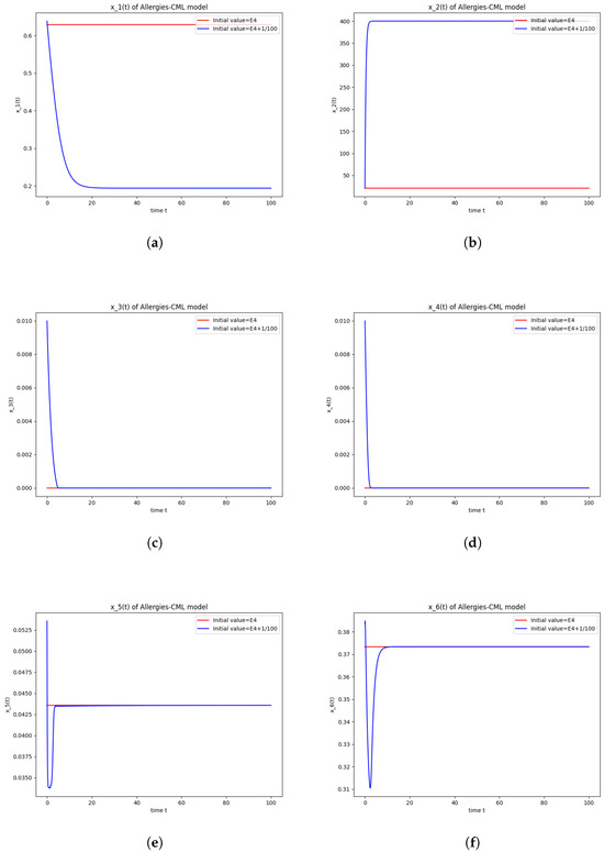
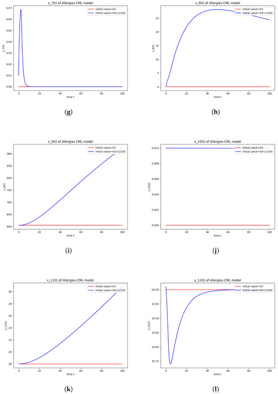
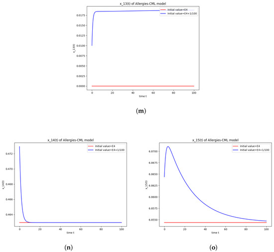
Figure 4.
Stability around the equilibrium point . (a) The concentration of stem-like healthy cells around . (b) The concentration of mature healthy cells around . (c) The concentration of stem-like leukemic cells around . (d) The concentration of mature leukemic cells around . (e) The concentration of naive APCs around . (f) The concentration of mature APCs activated by the drug around . (g) The concentration of mature APCs activated by the leukemic cells around . (h) The concentration of naive CD4+ T cells around . (i) The concentration of Th1 cells around . (j) The concentration of Th2 cells around . (k) The concentration of Treg cells around . (l) The concentration of naive CD8+ T cells around . (m) The concentration of mature CD8+ T cells around . (n) The amount of drug in the absorbtion compartment around . (o) The amount of drug in the plasmatic compartment around .
Our numerical simulations reveal several characteristics of immune dynamics during imatinib therapy:
- Simulations indicate that in some scenarios, the concentration of Th2 cells exceeds that of Th1 cells, leading to allergic reactions. In these cases, both healthy and leukemic cell populations diminish to zero.
- In other scenarios, while leukemic cells reduce to undetectable levels, healthy cells stabilize at positive values. However, an imbalance favoring Th2 cells still results in allergic reactions.
- Some simulations show a positive evolution with leukemic cells dying out and a rapid increase in Th1 cell concentration. Yet, high Th2 cell concentrations indicate persistent allergic reactions.
- Importantly, there are scenarios where leukemic cells are eliminated without triggering allergic reactions. In these cases, the concentration of Th1 cells greatly outnumbers Th2 cells, providing a more favorable therapeutic outcome.
6. Conclusions and Future Work
This article presents a mathematical model that describes the dynamics of both healthy and leukemic cells, along with the role of the immune system, in the context of Chronic Myeloid Leukemia (CML) under treatment. The goal is to study the occurrence of allergic reactions to imatinib treatment by investigating the underlying mechanism behind the dominance of Th2 cells over Th1 and Treg cells.
Delay differential equations were used because time delays aid in accurately capturing the timing of biological processes. The model offers detailed insights into the inner workings of the immune system, including the behavior and activation of the cells responsible for the immune response (APCs, CD4+ T cells, CD8+ T cells, Th1 cells, Th2 cells, Treg cells).
Demonstrating the positivity of solutions is crucial when dealing with variables that represent cell populations. Section 3 of this paper covers the problem of positivity. We successfully demonstrated that, when the initial data have positive values, the solutions will remain positive throughout.
We identified the potential equilibria of the system and conducted an exhaustive local stability analysis around these points. Section 4 provides the mathematical calculations and findings regarding the four distinct equilibrium points uncovered. Biologically, these correspond to the following scenarios: patient demise, a healthy condition, a cured state with allergic reactions, and a cured state without allergic reactions.
We performed numerical simulations for four equilibrium points. The first equilibrium point is unstable, which is desirable since it describes the death of the patient (or possibly the state immediately following a bone marrow transplant). Unfortunately, the evolution of healthy cells in this configuration is not favorable.
The second equilibrium point is also unstable. Nonetheless, the simulations describe a positive evolution where leukemic cell counts decrease to undetectable levels, and healthy cells gravitate towards a positive state. Despite starting with equivalent concentrations of Th1 and Th2 cells in simulations, the evolutionary trend demonstrates immunological destabilization, evidenced by a higher concentration of Th2 cells compared to Th1 cells. Thus, although the patient has a favorable evolution as the leukemic burden diminishes, we expect allergic reactions to appear.
The numerical computations and simulations conducted around the third equilibrium point suggest instability. Despite this, there is a positive trend observed as leukemic cells diminish and the concentration of Th1 cells experiences rapid growth. Allergic reactions persist due to the significant concentration of Th2 cells, which greatly surpasses that of Th1 cells. This situation may change, as there seems to be a decreasing trend in the population of Th2 cells.
The last equilibrium point is unstable, according to the numerical computations and simulations. The simulations show a promising evolution, with no allergic reactions.
While the current parameter configuration renders all equilibrium points unstable, we can detect partial stability in certain variables of the system. This paves the way for new mathematical studies aimed at exploring the circumstances under which specific variables remain stable independent of others.
Mathematically simulating allergic reactions in the context of drug allergies is a critical area of research that holds substantial importance in both pharmacology and clinical medicine. This approach offers multiple benefits, from enhancing our understanding of allergic mechanisms to improving patient safety. Based on the findings outlined in this article, the next step involves exploring various parameter scenarios to gain a holistic understanding of the correlation between drug concentration and the onset of allergic reactions.
In summary, this study aims to provide a nuanced understanding of the immune system’s behavior during CML therapy with imatinib. By addressing the current gaps in knowledge and offering a detailed mathematical framework, we hope to contribute to the development of more effective treatment strategies and the management of immune-related side-effects in CML patients.
Author Contributions
Conceptualization, R.A.; Validation, I.B.; Data curation, L.F.; Writing—original draft, R.A.; Writing—review & editing, R.A. and A.H. All authors have read and agreed to the published version of the manuscript.
Funding
This research received no external funding.
Data Availability Statement
The original contributions presented in the study are included in the article, further inquiries can be directed to the corresponding authors.
Conflicts of Interest
The authors declare no conflicts of interest.
Appendix A
In the following, the matrices of partial derivatives calculated in equilibria will be listed. Everywhere, the state variables are calculated in equilibria.
The equilibrium point .
The nonzero elements in A are:
The nonzero element in B is
The nonzero element in C is
The nonzero element in D is
The nonzero element in E is
The nonzero element in G is
The nonzero element in H is
F is zero.
The equilibrium point
The nonzero elements in A are:
The nonzero elements in B are:
The nonzero elements in C are:
The nonzero element in D is:
The nonzero element in E is:
The nonzero element in G is:
The nonzero element in H is:
The equilibrium point
The nonzero elements in A are:
The nonzero elements in B are:
The nonzero elements in C are:
The nonzero element in D is:
The nonzero element in E is:
The nonzero elements in F are:
The nonzero element in G is:
The nonzero elements in H are:
The equilibrium point
The nonzero elements in A are:
The nonzero elements in B are:
The nonzero elements in C are:
The nonzero element in D is:
The nonzero element in E is:
The nonzero elements in F are:
The nonzero elements in G is:
The nonzero elements in H are:
References
- Adimy, M.; Crauste, F.; Ruan, S. A mathematical study of the hematopoiesis process with application to chronic myelogenous leukemia. SIAM J. Appl. Math. 2005, 65, 1328–1352. [Google Scholar] [CrossRef]
- Colijn, C.; Mackey, M.C. A mathematical model of hematopoiesis I-Periodic chronic myelogenous leukemia. J. Theor. Biol. 2005, 237, 117–132. [Google Scholar] [CrossRef] [PubMed]
- Badralexi, I.; Halanay, A. A Complex Model for Blood Cells’ Evolution in Chronic Myelogenous Leukemia. In Proceedings of the 20th International Conference on Control Systems and Computer Science (CSCS), Bucharest, Romania, 27–29 May 2015; pp. 611–617. [Google Scholar]
- Radulescu, R.; Candea, D.; Halanay, A. Stability and bifurcation in a model for the dynamics of stem-like cells in leukemia under treatment. Am. Inst. Phys. Proc. 2012, 1493, 758–763. [Google Scholar]
- Halanay, A.; Cândea, D.; Rădulescu, I.R. Existence and Stability of Limit Cycles in a Two Delays Model of Hematopoietis Including Asymmetric Division. Math. Model. Nat. Phen. 2014, 9, 58–78. [Google Scholar] [CrossRef]
- Badralexi, I.; Candea, D.; Halanay, A.; Radulescu, I.R. A model for cell evolution in CML under treatment including pharmakodynamics. Bull. Math. Soc. Sci. Math. Roum. 2018, 61, 383–398. [Google Scholar]
- Badralexi, I.; Halanay, A. Stability and oscillations in a CML model. AIP Conf. Proc. 2017, 1798, 020011. [Google Scholar]
- Balea, S.; Halanay, A.; Neamtu, M. A feedback model for leukemia including cell competition and the action of the immune system. AIP Conf. Proc. 2014, 1637, 1316–1324. [Google Scholar]
- Kim, P.; Lee, P.; Levy, D. Dynamics and Potential Impact of the Immune Response to Chronic Myelogenous Leukemia. PLoS Comput. Biol. 2008, 4, e1000095. [Google Scholar] [CrossRef] [PubMed]
- Michor, F.; Hughes, T.; Iwasa, Y.; Branford, S.; Shah, N.P.; Sawyers, C.; Novak, M. Dynamics of chronic myeloid leukemia. Nature 2005, 435, 1267–1270. [Google Scholar] [CrossRef]
- Moore, H.; Li, N.K. A mathematical model for chronic myelogenous leukemia (CML) and T-cell interaction. J. Theor. Biol. 2004, 227, 513–523. [Google Scholar] [CrossRef]
- Peet, M.M.; Kim, P.S.; Niculescu, S.I.; Levy, D. New Computational Tools for Modeling Chronic Myelogenous Leukemia. Math. Model. Nat. Phenom. 2009, 4, 48–68. [Google Scholar] [CrossRef][Green Version]
- Pujo-Menjouet, L.; Mackey, M.C. Contribution to the study of periodic chronic myelogenous leukemia. Comptes Rendus Biol. 2004, 327, 235–244. [Google Scholar] [CrossRef] [PubMed]
- Gross, F.; Metzner, G.; Behn, U. Mathematical modeling of allergy and specific immunotherapy: Th1, Th2 and Treg interactions. J. Theor. Biol. 2011, 269, 70–78. [Google Scholar] [CrossRef] [PubMed]
- Abdullah, R.; Amin, K.; Halanay, A.; Mghames, R. Partial stability in a model for allergic reactions induced by chemotherapy of acute lymphoblastic leukemia. Ann. Ser. Math. Its Appl. 2023, 15, 443. [Google Scholar] [CrossRef]
- Behn, U.; Dambeck, H.; Metzner, G. Modeling th1-th2 regulation, allergy, and hyposensitization. In Dynamical Modeling in Biotechnology: Lectures Presented at the EU Advanced Workshop; World Scientic: Singapore, 2001; pp. 227–243. [Google Scholar]
- Segel, L.A.; Fishman, M.A. Modeling immunotherapy for allergy. Bull. Math. Biol. 1996, 58, 1099–1121. [Google Scholar]
- Klaewsongkram, J.; Thantiworasit, M.P.; Sodsai, P.; Buranapraditkun, S.; Mongkolpathumrat, P. Slow desensitization of imatinib-induced nonimmediate reactions and dynamic changes of drug-specific CD4+ CD25+ CD134+ lymphocytes. Ann. Allergy Asthma Immunol. 2016, 117, 514–519. [Google Scholar] [CrossRef] [PubMed]
- Kim, P.; Lee, P.; Levy, D. A theory of immunodominance and adaptive regulation. Bull. Math. Biol. 2011, 73, 1645–1665. [Google Scholar] [CrossRef] [PubMed]
- Dai, J.Y.; Yang, X.; Wei, Q.; I, H.L.; Huang, X.B.; Wang, X.B. Effects of Tyrosine Kinase Inhibitors on the Th1 and Treg Cells of CML Patients. J. Exp. Hematol. 2019, 27, 25–32. [Google Scholar]
- Widmer, N.; Decosterd, L.A.; Csajka, C.; Leyvraz, S.; Duchosal, M.A.; Rosselet, A.; Rochat, B.; Eap, C.B.; Henry, H.; Biollaz, J.; et al. Population pharmacokinetics of imatinib and the role of pm 1-acid glycoprotein. Br. J. Clin. Pharmacol. 2006, 62, 97–112. [Google Scholar] [CrossRef] [PubMed]
- Wu, G. Calculation of steady-state distribution delay between central and peripheral compartments in two-compartment models with infusion regimen. Eur. J. Drug Metab. Pharmacokinet. 2002, 27, 259–264. [Google Scholar] [CrossRef]
- Bellman, R.; Cooke, K.L. Differential-Difference Equations; Academic Press: New York, NY, USA, 1963. [Google Scholar]
- Cooke, K.; Grossman, Z. Discrete Delay, Distribution Delay and Stability Switches. J. Math. Anal. Appl. 1982, 86, 592–627. [Google Scholar] [CrossRef]
- Wang, X.; Kottegoda, C.; Shan, C.; Huang, Q. Oscillations and coexistence generated by discrete delays in a two-species competition model. Discret. Contin. Dyn. Syst. B 2024, 29, 1798–1814. [Google Scholar] [CrossRef]
- Cooke, K.; van den Driessche, P. On zeros of some transcendental equations. Funkc. Ekvacioj 1986, 29, 77–90. [Google Scholar]
- Kogan, Y.; Agur, Z.; Elishmereni, M. A mathematical model for the immunotherapeutic control of the TH1/TH2 imbalance in melanoma. Discret. Contin. Dyn. Syst. B 2013, 18, 1017–1030. [Google Scholar] [CrossRef]
- Gil, W.; Carvalho, T.; Mancera, P.; Rodrigues, D.S. A Mathematical Model on the Immune System Role in Achieving Better Outcomes of Cancer Chemotherapy. Trends Comput. Appl. Math. 2019, 20, 343–357. [Google Scholar] [CrossRef]


Disclaimer/Publisher’s Note: The statements, opinions and data contained in all publications are solely those of the individual author(s) and contributor(s) and not of MDPI and/or the editor(s). MDPI and/or the editor(s) disclaim responsibility for any injury to people or property resulting from any ideas, methods, instructions or products referred to in the content. |
© 2024 by the authors. Licensee MDPI, Basel, Switzerland. This article is an open access article distributed under the terms and conditions of the Creative Commons Attribution (CC BY) license (https://creativecommons.org/licenses/by/4.0/).