
Modeling Data with Extreme Values Using Three-Spliced Distributions


Abstract
:1. Introduction
2. Three-Component Spliced Distributions
2.1. General Form
- (a)
- Imposing continuity conditions at the thresholds , i.e., yields
- (b)
- The proof can be found in [22]. □
2.2. Parameter Estimation
- Step 1.
- Select the initial values for the thresholds (using, for example, graphical diagnostics) and, for each threshold, set up a search grid around its initial value.
- Step 2.
- For in its gridFor in its gridEvaluate the remaining parameters by MLE of the likelihood (5) under the constraints of continuity at the thresholds and differentiability if considered.
- Step 3.
- Among the solutions obtained at Step 2, choose the one that maximizes the log-likelihood function.
- Step 4.
- The algorithm can be reiterated by refining the grids around the last threshold values.
2.3. Particular Involved Distributions
3. Numerical Illustration
4. Conclusions and Future Work
Author Contributions
Funding
Data Availability Statement
Acknowledgments
Conflicts of Interest
Appendix A. Tables

| Head | Middle | Tail | , | |
|---|---|---|---|---|
| Weibull 13.301, 5.696 (0.818, 2.966 ) | LogLogistic 0.434, 0.027 (0.629, 0.376) | Pareto a = 1.414 (0.037) | 0.925 1.612 | 0.063, 0.432 0.505 |
| Weibull 14.625, 1.412 (0.995, 0.894) | Weibull 0.891,1.033 (0.631, 0.318) | Pareto a = 1.416 (0.038) | 0.908 1.607 | 0.053, 0.439 0.508 |
| LogNormal 34.971, 1.563 (36.022, 0.799) | Weibull 1.357, 1.144 (0.159, 0.092) | Pareto a = 1.372 (0.048) | 0.908 2.381 | 0.053, 0.661 0.286 |
| Weibull 14.469, 3.349 (0.981, 1.048 ) | Weibull 1.449, 1.168 (0.168, 0.083) | InverseWeibull 1.487, 1.036 (0.096, 0.547) | 0.907 2.380 | 0.052, 0.660 0.288 |
| Weibull 13.170, 1.307 (0.798, 9.987) | LogLogistic 0.494, 0.039 (0.157, 0.016) | InverseParalogistic 1.414, 0.010 (0.037, 8.948 ) | 0.928 1.630 | 0.065, 0.437 0.498 |
| Weibull 13.126, 1.434 (0.924, 1.286) | Paralogistic 0.760, 0.202 (1.924, 3.421) | LogLogistic 1.413, 4.791 (0.037, 8.948 ) | 0.928 1.611 | 0.064, 0.431 0.505 |
| Weibull 13.195, 2.161 (0.805, 26.465) | Paralogistic 0.551, 1.239 (0.109, 8.948 ) | InverseWeibull 1.413, 1.177 (3.932 , 0.301) | 0.927 1.607 | 0.064, 0.429 0.507 |
| LogNormal 37.297, 1.618 (61.381, 1.180) | Weibull 1.438, 1.166 (0.156, 0.080) | InverseParalogistic 1.501, 0.666 (0.099, 0.323) | 0.908 2.422 | 0.053, 0.666 0.281 |
| Weibull 13.183, 1.533 (0.804, 1.954) | LogLogistic 1.806, 0.894 (0.088, 0.084) | InverseWeibull 2.022, 10.462 (0.240, 1.291) | 0.928 9.506 | 0.065, 0.890 0.045 |
| Weibull 15.881, 1.875 (1.169, 11.988) | Paralogistic 2.154, 1.745 (0.157, 0.089) | InverseParalogistic 1.483, 0.544 (0.098, 0.335) | 0.891 2.350 | 0.044, 0.662 0.294 |
| LogNormal 20.985, 1.231 (18.962, 0.546) | Weibull 1.329, 1.120 (0.159, 0.097) | LogLogistic 1.454, 0.564 (0.103, 0.470) | 0.912 2.467 | 0.056, 0.670 0.274 |
| Paralogistic 15.860, 1.649 (1.180, 0.938) | LogLogistic 2.670, 1.205 (0.221, 0.047) | InverseWeibull 1.478, 0.930 (0.098, 0.596) | 0.891 2.474 | 0.043, 0.682 0.275 |
| Weibull 15.808, 7.666 (1.178, 2.965 ) | LogLogistic 2.700, 1.206 (0.230, 0.046) | LogLogistic 1.473, 0.558 (0.100, 0.429) | 0.891 2.399 | 0.043, 0.670 0.287 |
| Weibull 13.254, 5.734 (0.839, 2.097 ) | Weibull 0.362, 0.417 (0.615, 1.469) | LogLogistic 1.408, 0.050 (0.074, 0.377) | 0.924 1.529 | 0.062, 0.398 0.540 |
| LogLogistic 13.775, 7.703 (0.858, 2.965 ) | LogLogistic 1.834, 0.928 (0.088, 0.081) | InverseWeibull 1.990, 10.049 (0.233, 1.283) | 0.920 9.216 | 0.061, 0.893 0.046 |
| LogNormal 11.608, 0.960 (8.851, 0.356) | Weibull 1.231, 1.039 (0.156, 0.114) | InverseWeibull 1.556, 1.553 (0.094, 0.463) | 0.928 2.586 | 0.064, 0.677 0.259 |
| Paralogistic 15.145, 3.873 (0.905, 0.498) | Paralogistic 1.867, 1.593 (0.115, 0.116) | LogLogistic 1.524, 1.018 (0.115, 0.541) | 0.901 2.914 | 0.050, 0.732 0.218 |
| Paralogistic 1.082, 0.964 (0.127,0.120) | Weibull 13.417, 7.272 (0.016, 0.015) | InverseWeibull 1.540, 1.617 (0.106, 0.611) | 0.922 2.888 | 0.061, 0.718 0.221 |
| Weibull 13.682, 1.858 (0.841, 7.220) | InverseBurr 3.833 , 6.060, 2.261 (8.948 , 1.397, 0.051) | InverseParalogistic 1.494, 0.638 (0.097, 0.324) | 0.917 2.309 | 0.059, 0.642 0.299 |
| Weibull 14.443, 2.939 (0.963, 432.610) | InverseBurr 0.027, 4.704, 2.203 (0.079, 1.536, 0.221) | LogLogistic 1.448, 0.438 (0.103, 0.479) | 0.912 2.295 | 0.055, 0.642 0.303 |
| Weibull 15.309, 1.469 (1.076, 1.339) | InverseBurr 0.103, 4.120, 2.043 (0.145, 1.204, 0.311) | InverseWeibull 1.506, 1.200 (0.095, 0.517) | 0.901 2.419 | 0.049, 0.669 0.282 |
| InverseBurr 6.594, 2.399, 5.262 (5.201, 1.830, 4.813) | LogLogistic 2.623, 1.202 (0.245, 0.049) | InverseWeibull 1.418, 0.442 (0.121, 1.013) | 0.893 2.426 | 0.045, 0.674 0.281 |
| Head | Middle | Tail | , | |
|---|---|---|---|---|
| Weibull 16.452, 0.946 (0.884, —) | LogLogistic 2.338, 1.112 (0.111, —) | Pareto a = 1.410 (0.036) | 0.944 2.022 | 0.081, 0.552 0.367 |
| Weibull 16.300, 0.948 (0.853, —) | Weibull 1.335,1.088 (0.124, —) | Pareto a = 1.410 (0.037) | 0.947 1.867 | 0.083, 0.507 0.410 |
| LogNormal 0.096, 0.179 (—, 0.007) | Weibull 0.970, 0.810 (0.136, —) | Pareto a = 1.409 (0.039) | 1.025 2.041 | 0.144, 0.494 0.362 |
| Weibull 16.841, 0.941 (0.818, —) | Weibull 1.474, 1.141 (1.001 , 1.001 ) | InverseWeibull 1.406, 3.881 (1.001 , —) | 0.940 1.797 | 0.078, 0.490 0.432 |
| Weibull 16.604, 0.944 (0.901, —) | LogLogistic 2.363, 1.120 (0.112, —) | InverseParalogistic 1.411, 1.764 (0.036, 8.948 ) | 0.942 2.007 | 0.079, 0.550 0.371 |
| Weibull 16.318, 0.947 (0.773, —) | Paralogistic 1.884, 1.546 (8.948 , 8.948 ) | LogLogistic 1.410, 7.320 (8.948 , —) | 0.946 1.945 | 0.082, 0.530 0.388 |
| Weibull 16.893, 0.940 (0.948, —) | Paralogistic 2.041, 1.632 (0.166, 0.118) | InverseWeibull 1.415, 0.154 (0.072, —) | 0.938 1.799 | 0.077, 0.492 0.431 |
| LogNormal 0.112, 0.184 (—, 7.636 ) | Weibull 0.749, 0.557 (0.113, —) | InverseParalogistic 1.420, 3.600 (0.041, 1.001 ) | 1.030 2.302 | 0.148, 0.545 0.307 |
| Weibull 15.979, 0.951 (0.738, —) | LogLogistic 2.148, 1.058 (8.948 , 8.948 ) | InverseWeibull 1.427, 1.154 (8.948 , —) | 0.950 2.230 | 0.086, 0.594 0.320 |
| Weibull 16.422, 0.946 (0.870, —) | Paralogistic 1.885, 1.548 (0.088,—) | InverseParalogistic 1.412, 4.156 (0.037, 8.948) | 0.945 1.946 | 0.082, 0.531 0.387 |
| LogNormal 0.104, 0.182 (—, 7.416 ) | Weibull 0.979, 0.813 (0.141, —) | LogLogistic 1.409, 1.322 (0.039, 1.001 ) | 1.030 2.021 | 0.147, 0.486 0.367 |
| Paralogistic 15.571, 1.145 (8.948 , 8.948 ) | LogLogistic 2.139, 1.040 (8.948 , —) | InverseWeibull 1.416, 1.254 (8.948 , —) | 0.959 2.189 | 0.091, 0.580 0.329 |
| Weibull 16.515, 0.945 (0.893, —) | LogLogistic 2.360, 1.118 (0.112, —) | LogLogistic 1.410, 2.013 (0.036, 8.948 ) | 0.943 2.005 | 0.080, 0.549 0.371 |
| Weibull 16.231, 0.949 (0.844, —) | Weibull 1.296, 1.073 (0.121, —) | LogLogistic 1.412, 5.428 (0.037, 1.001 ) | 0.948 1.895 | 0.084, 0.514 0.402 |
| LogLogistic 16.577, 0.965 (0.718, —) | LogLogistic 2.325, 1.099 (0.035, 8.948 ) | InverseWeibull 1.407, 2.408 (0.035, —) | 0.963 2.009 | 0.095, 0.535 0.370 |
| LogNormal 0.104, 0.182 (—, 7.334 ) | Weibull 0.977, 0.810 (8.948 , 8.948 ) | InverseWeibull 1.408, 1.453 (8.948 , —) | 1.030 2.022 | 0.147, 0.487 0.366 |
| Paralogistic 16.278, 1.127 (0.754, —) | Paralogistic 1.864, 1.531 (8.948 , 8.948 ) | LogLogistic 1.412, 3.506 (8.948 , —) | 0.948 1.962 | 0.084, 0.533 0.383 |
| Paralogistic 11.533, 1.389 (0.815, 0.148) | Weibull 14.359, 0.989 (0.693, —) | InverseWeibull 1.537, 0.830 (0.049, —) | 0.902 0.991 | 0.045, 0.070 0.885 |
| Weibull 15.747, 0.955 (0.806, —) | InverseBurr 0.057, 3.466, 2.089 (—, 0.864, 0.376) | InverseParalogistic 1.421, 1.214 (0.038, 8.948 ) | 0.955 1.953 | 0.090, 0.525 0.385 |
| Weibull 17.828, 0.932 (1.038, —) | InverseBurr 0.049, 6.765, 1.906 (—, 4.658, 0.092) | LogLogistic 1.413, 0.114 (0.080, 0.317) | 0.931 1.603 | 0.073, 0.423 0.504 |
| Weibull 15.832, 0.954 (0.874, —) | InverseBurr 0.291, 2.761, 1.651 (—, 1.137, 1.123) | InverseWeibull 1.413, 5.797 (0.042, 8.948 ) | 0.953 1.977 | 0.087, 0.534 0.379 |
| InverseBurr 0.592, 23.222, 0.993 (—, 4.265, 7.457 ) | LogLogistic 1.702, 0.797 (8.948 , 8.948 ) | InverseWeibull 1.463, 3.400 (8.948 , —) | 0.972 3.633 | 0.103, 0.735 0.162 |
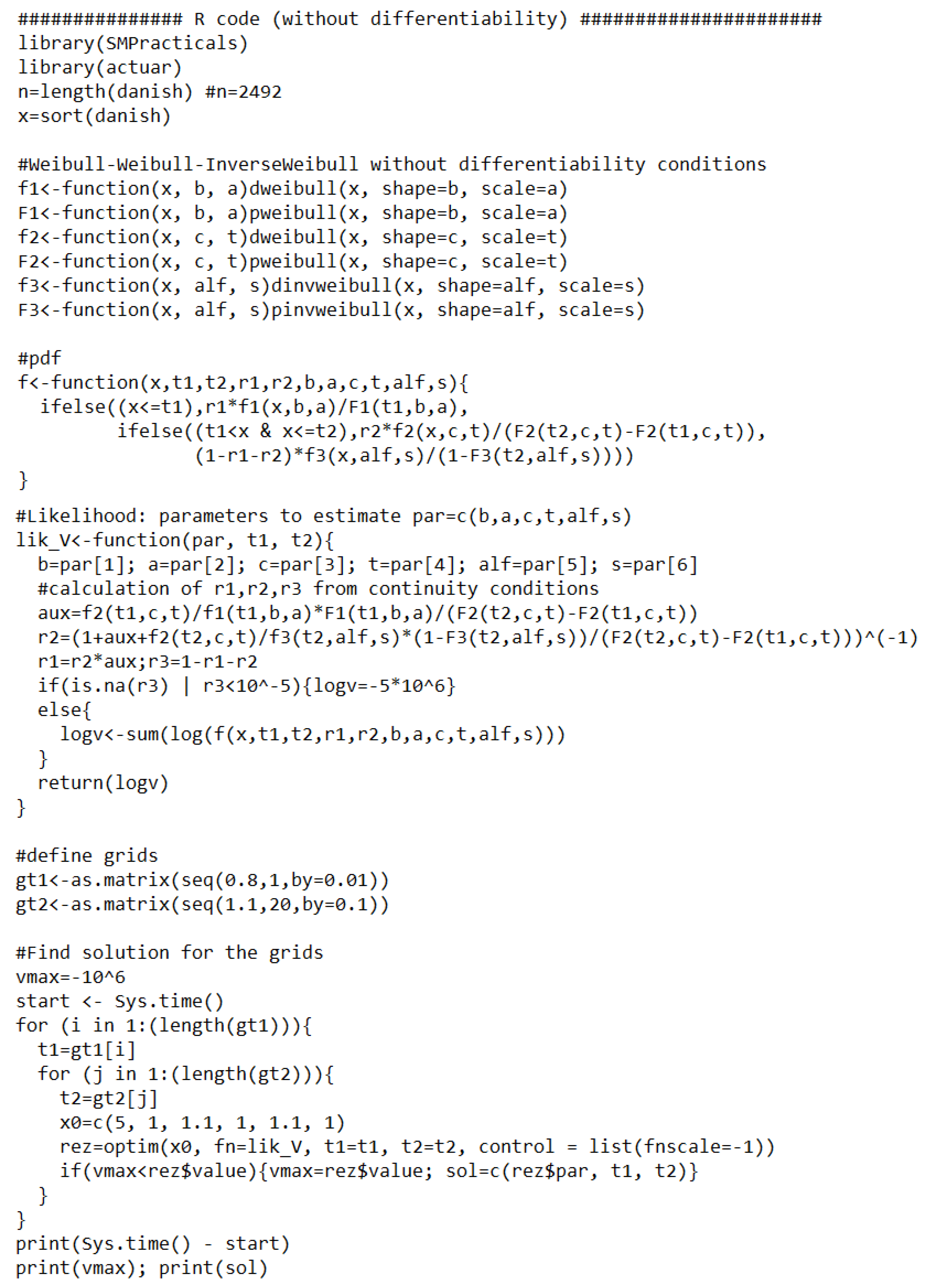
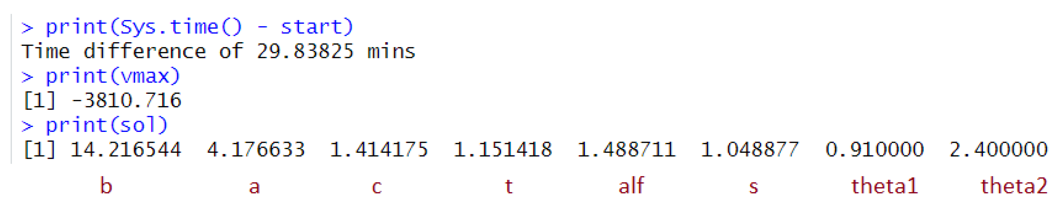
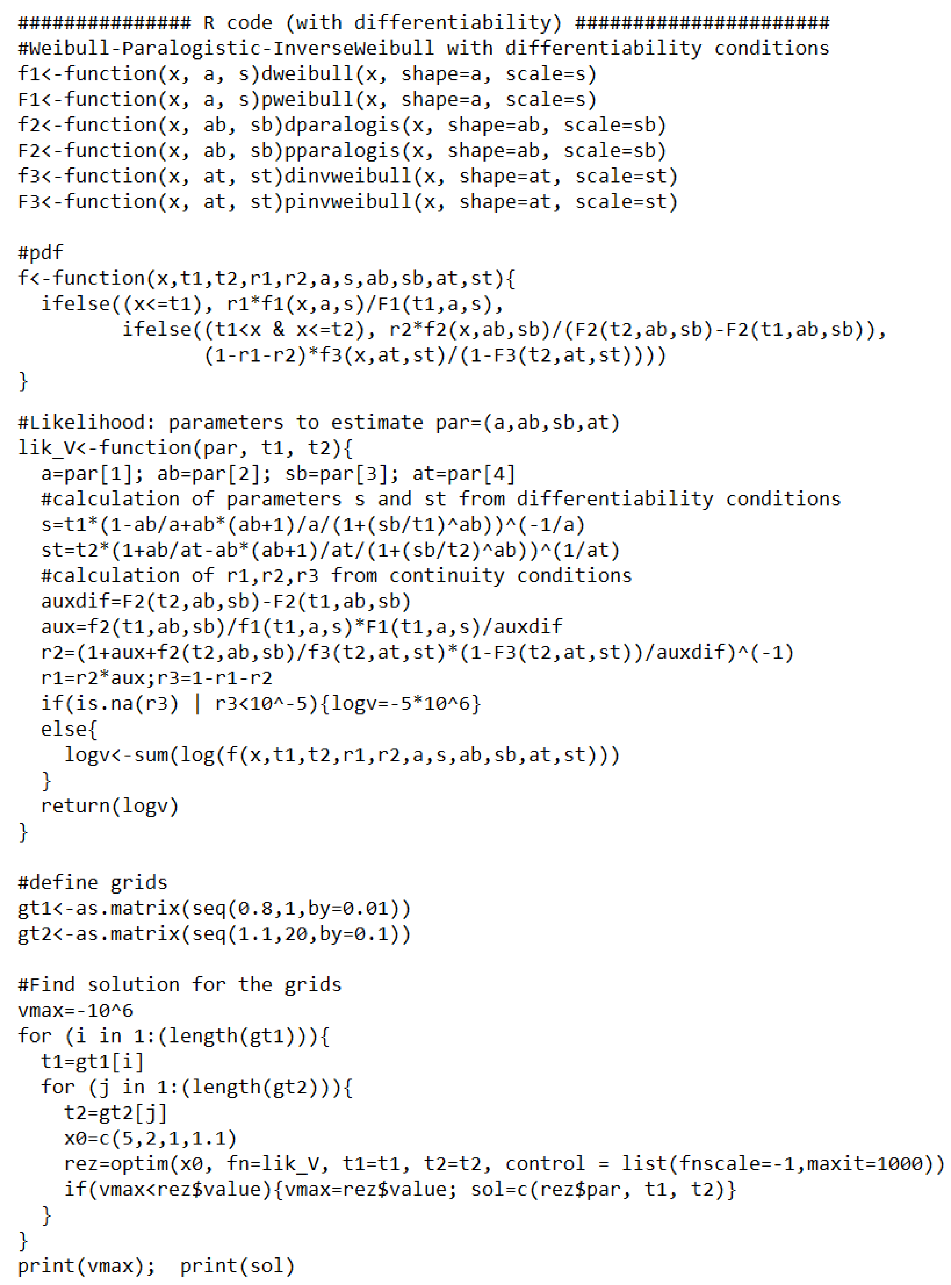
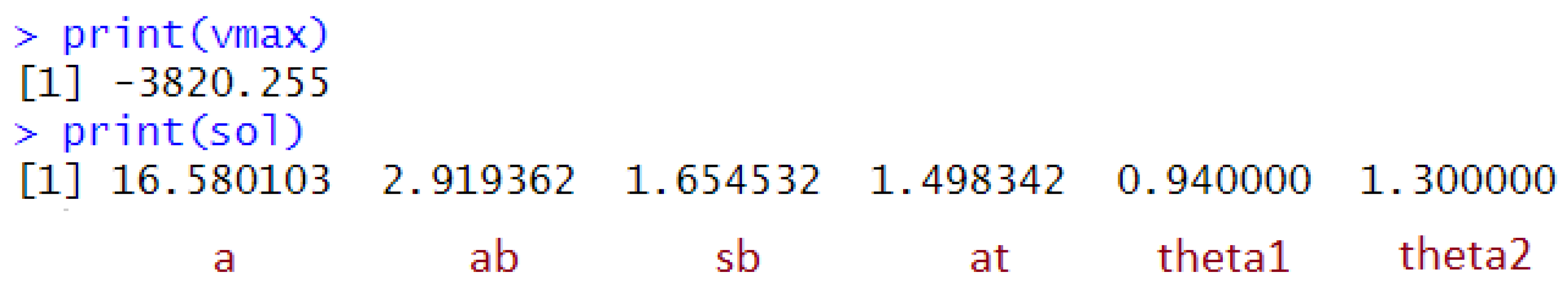
Appendix B. R Code
References
- Klugman, S.A.; Panjer, H.H.; Willmot, G.E. Loss Models: From Data to Decisions; John Wiley & Sons: Hoboken, NJ, USA, 2012; Volume 715. [Google Scholar]
- Cooray, K.; Ananda, M.M. Modeling actuarial data with a composite lognormal-Pareto model. Scand. Actuar. J. 2005, 2005, 321–334. [Google Scholar] [CrossRef]
- Scollnik, D.P. On composite lognormal-Pareto models. Scand. Actuar. J. 2007, 2007, 20–33. [Google Scholar] [CrossRef]
- Bakar, S.A.; Hamzah, N.A.; Maghsoudi, M.; Nadarajah, S. Modeling loss data using composite models. Insur. Math. Econ. 2015, 61, 146–154. [Google Scholar] [CrossRef]
- Calderin-Ojeda, E. On the Composite Weibull–Burr Model to describe claim data. Commun. Stat. Case Stud. Data Anal. Appl. 2015, 1, 59–69. [Google Scholar] [CrossRef]
- Calderin-Ojeda, E.; Kwok, C.F. Modeling claims data with composite Stoppa models. Scand. Actuar. J. 2016, 2016, 817–836. [Google Scholar] [CrossRef]
- Grün, B.; Miljkovic, T. Extending composite loss models using a general framework of advanced computational tools. Scand. Actuar. J. 2019, 2019, 642–660. [Google Scholar] [CrossRef]
- Marambakuyana, W.A.; Shongwe, S.C. Composite and Mixture Distributions for Heavy-Tailed Data—An Application to Insurance Claims. Mathematics 2024, 12, 335. [Google Scholar] [CrossRef]
- Mutali, S.; Vernic, R. On the composite Lognormal–Pareto distribution with uncertain threshold. Commun.-Stat.-Simul. Comput. 2020, 51, 4492–4508. [Google Scholar] [CrossRef]
- Nadarajah, S.; Bakar, S. New composite models for the Danish fire insurance data. Scand. Actuar. J. 2014, 2014, 180–187. [Google Scholar] [CrossRef]
- Reynkens, T.; Verbelen, R.; Beirlant, J.; Antonio, K. Modelling censored losses using splicing: A global fit strategy with mixed Erlang and extreme value distributions. Insur. Math. Econ. 2017, 77, 65–77. [Google Scholar] [CrossRef]
- Scollnik, D.P.; Sun, C. Modeling with Weibull-Pareto models. N. Am. Actuar. J. 2012, 16, 260–272. [Google Scholar] [CrossRef]
- Abdul Majid, M.H.; Ibrahim, K. On Bayesian approach to composite Pareto models. PLoS ONE 2021, 16, e0257762. [Google Scholar] [CrossRef]
- Aradhye, G.; Tzougas, G.; Bhati, D. A Copula-Based Bivariate Composite Model for Modelling Claim Costs. Mathematics 2024, 12, 350. [Google Scholar] [CrossRef]
- Calderín-Ojeda, E.; Gómez-Déniz, E.; Vázquez-Polo, F.J. Conditional tail expectation and premium calculation under asymmetric loss. Axioms 2023, 12, 496. [Google Scholar] [CrossRef]
- Fung, T.C.; Tzougas, G.; Wüthrich, M.V. Mixture composite regression models with multi-type feature selection. N. Am. Actuar. J. 2023, 27, 396–428. [Google Scholar] [CrossRef]
- Liu, B.; Ananda, M.M. A generalized family of exponentiated composite distributions. Mathematics 2022, 10, 1895. [Google Scholar] [CrossRef]
- Liu, B.; Ananda, M.M. A new insight into reliability data modeling with an exponentiated composite Exponential-Pareto model. Appl. Sci. 2023, 13, 645. [Google Scholar] [CrossRef]
- Scarrott, C. Univariate extreme value mixture modeling. In Extreme Value Modeling and Risk Analysis; Taylor & Francis: London, UK, 2016; pp. 41–67. [Google Scholar]
- Fang, K.; Ma, S. Three-part model for fractional response variables with application to Chinese household health insurance coverage. J. Appl. Stat. 2013, 40, 925–940. [Google Scholar] [CrossRef]
- Gan, G.; Valdez, E.A. Fat-tailed regression modeling with spliced distributions. N. Am. Actuar. J. 2018, 22, 554–573. [Google Scholar] [CrossRef]
- Baca, A.; Vernic, R. On the three-spliced Exponential-Lognormal-Pareto distribution. Analele ştiinţifice ale Universităţii Ovidius Constanţa. Ser. Mat. 2022, 30, 21–35. [Google Scholar]
- Baca, A.; Vernic, R. Extreme values modeling using the Gamma-Lognormal-Pareto three-spliced distribution. In Changes and Innovations in Social Systems: 505 (Studies in Systems, Decision and Control); Hoskova-Mayerova, S., Flaut, C., Flaut, D., Rackova, P., Eds.; Springer: Berlin/Heidelberg, Germany, 2024. [Google Scholar]
- Li, J.; Liu, J. Claims Modelling with Three-Component Composite Models. Risks 2023, 11, 196. [Google Scholar] [CrossRef]
- Majid, M.H.A.; Ibrahim, K.; Masseran, N. Three-Part Composite Pareto Modelling for Income Distribution in Malaysia. Mathematics 2023, 11, 2899. [Google Scholar] [CrossRef]
- Nelder, J.A.; Mead, R. A simplex algorithm for function minimization. Comput. J. 1965, 7, 308–313. [Google Scholar] [CrossRef]
| Distribution | Density |
|---|---|
| Inverse Burr (IB) | |
| Inverse Paralogistic (IP) | |
| Inverse Weibull (IW) | |
| LogLogistic (LL) | |
| LogNormal (LN) | |
| Paralogistic (P) | |
| Pareto (Pa) | |
| Weibull (W) |
| Mean | Std | Min | Q25 | Median | Q75 | Max | Kurtosis | Skewness |
|---|---|---|---|---|---|---|---|---|
| 3.063 | 7.977 | 0.313 | 1.157 | 1.634 | 2.645 | 263.250 | 549.574 | 19.896 |
| Head | Middle | Tail | Diff. | NLL | k | AIC | BIC | Rank | |
|---|---|---|---|---|---|---|---|---|---|
| 1 | Weibull | LogLogistic | Pareto | No | 3810.93 | 5 | 7631.86 | 7660.97 | 3 |
| Yes | 3816.16 | 3 | 7638.33 | 7655.79 | 2 | ||||
| 2 | Weibull | Weibull | Pareto | No | 3811.58 | 5 | 7633.16 | 7662.26 | 5 |
| Yes | 3815.50 | 3 | 7637.00 | 7654.46 | 1 | ||||
| 3 | LogNormal | Weibull | Pareto | No | 3811.86 | 5 | 7633.72 | 7662.83 | 6 |
| Yes | 3854.34 | 3 | 7714.68 | 7732.14 | 41 | ||||
| 4 | Weibull | Weibull | InverseWeibull | No | 3810.57 | 6 | 7633.14 | 7668.06 | 17 |
| Yes | 3815.87 | 4 | 7639.74 | 7663.02 | 9 | ||||
| 5 | Weibull | LogLogistic | InverseParalogistic | No | 3810.69 | 6 | 7633.39 | 7668.31 | 18 |
| Yes | 3816.22 | 4 | 7640.45 | 7663.73 | 12 | ||||
| 6 | Weibull | Paralogistic | LogLogistic | No | 3810.71 | 6 | 7633.43 | 7668.35 | 19 |
| Yes | 3815.83 | 4 | 7639.67 | 7662.95 | 7 | ||||
| 7 | Weibull | Paralogistic | InverseWeibull | No | 3810.74 | 6 | 7633.47 | 7668.40 | 20 |
| Yes | 3816.44 | 4 | 7640.88 | 7664.16 | 14 | ||||
| 8 | LogNormal | Weibull | InverseParalogistic | No | 3811.03 | 6 | 7634.06 | 7668.99 | 21 |
| Yes | 3854.70 | 4 | 7717.41 | 7740.69 | 44 | ||||
| 9 | Weibull | LogLogistic | InverseWeibull | No | 3811.10 | 6 | 7634.20 | 7669.13 | 22 |
| Yes | 3816.43 | 4 | 7640.87 | 7664.15 | 13 | ||||
| 10 | Weibull | Paralogistic | InverseParalogistic | No | 3811.24 | 6 | 7634.49 | 7669.41 | 23 |
| Yes | 3815.85 | 4 | 7639.69 | 7662.97 | 8 | ||||
| 11 | LogNormal | Weibull | LogLogistic | No | 3811.66 | 6 | 7635.32 | 7670.24 | 25 |
| Yes | 3854.28 | 4 | 7716.56 | 7739.84 | 42 | ||||
| 12 | Paralogistic | LogLogistic | InverseWeibull | No | 3811.76 | 6 | 7635.52 | 7670.44 | 26 |
| Yes | 3816.78 | 4 | 7641.57 | 7664.85 | 15 | ||||
| 13 | Weibull | LogLogistic | LogLogistic | No | 3811.77 | 6 | 7635.54 | 7670.47 | 27 |
| Yes | 3816.19 | 4 | 7640.38 | 7663.66 | 11 | ||||
| 14 | Weibull | Weibull | LogLogistic | No | 3811.81 | 6 | 7635.61 | 7670.54 | 28 |
| Yes | 3815.48 | 4 | 7638.96 | 7662.24 | 4 | ||||
| 15 | LogLogistic | LogLogistic | InverseWeibull | No | 3811.81 | 6 | 7635.63 | 7670.55 | 29 |
| Yes | 3817.94 | 4 | 7643.87 | 7667.16 | 16 | ||||
| 16 | LogNormal | Weibull | InverseWeibull | No | 3812.20 | 6 | 7636.39 | 7671.32 | 31 |
| Yes | 3854.28 | 4 | 7716.56 | 7739.85 | 43 | ||||
| 17 | Paralogistic | Paralogistic | LogLogistic | No | 3812.31 | 6 | 7636.63 | 7671.55 | 32 |
| Yes | 3815.98 | 4 | 7639.96 | 7663.25 | 10 | ||||
| 18 | Paralogistic | Weibull | InverseWeibull | No | 3812.42 | 6 | 7636.84 | 7671.76 | 33 |
| Yes | 3823.83 | 4 | 7655.66 | 7678.94 | 39 | ||||
| 19 | Weibull | InverseBurr | InverseParalogistic | No | 3809.81 | 7 | 7633.61 | 7674.36 | 35 |
| Yes | 3815.50 | 5 | 7641.00 | 7670.11 | 24 | ||||
| 20 | Weibull | InverseBurr | LogLogisticAAAA | No | 3810.29 | 7 | 7634.59 | 7675.33 | 36 |
| Yes | 3817.38 | 5 | 7644.77 | 7673.87 | 34 | ||||
| 21 | Weibull | InverseBurr | InverseWeibull | No | 3810.61 | 7 | 7635.21 | 7675.96 | 38 |
| Yes | 3815.78 | 5 | 7641.56 | 7670.66 | 30 | ||||
| 22 | InverseBurr | LogLogistic | InverseWeibull | No | 3812.25 | 7 | 7638.51 | 7679.25 | 40 |
| Yes | 3818.36 | 5 | 7646.72 | 7675.82 | 37 |
| Head | Middle | Tail | NLL | k | AIC | BIC | KS | p-Value |
|---|---|---|---|---|---|---|---|---|
| Weibull | Paralogistic | LogLogistic | 3151.51 | 6 | 6315.03 | 6349.95 | 0.2689 | <2.2 |
| 11.802, 2.431 | 2.48 , 1.043 | 1.555, 5.419 | ||||||
| 0.078, 0.332, 0.590 | ||||||||
| Paralogistic | Paralogistic | LogLogistic | 3744.12 | 6 | 7500.24 | 7535.16 | 0.0477 | 2.3 |
| 10.370, 31.671 | 1.205, 0.329 | 1.521, 1.055 | ||||||
| 0.066, 0.826, 0.108 | ||||||||
| Paralogistic | Weibull | InverseWeibull | 3748.95 | 6 | 7509.91 | 7544.83 | 0.0450 | 8.2 |
| 11.497, 21.921 | 0.344, 0.034 | 1.334, 0.850 | ||||||
| 0.055, 0.901, 0.044 | ||||||||
| Paralogistic | LogLogistic | InverseWeibull | 3750.89 | 6 | 7513.78 | 7548.70 | 0.0689 | 1.0 |
| 9.309, 50.036 | 1.412, 0.354 | 1.664, 4.692 | ||||||
| 0.074, 0.899, 0.027 |
| Head | Tail | NLL | k | AIC | BIC |
|---|---|---|---|---|---|
| Weibull | InverseWeibull | 3820.01 | 4 | 7648.02 | 7671.30 |
| Paralogistic | InverseWeibull | 3820.14 | 4 | 7648.28 | 7671.56 |
| InverseBurr | InverseWeibull | 3816.34 | 5 | 7642.68 | 7671.79 |
| Weibull | InverseParalogistic | 3820.93 | 4 | 7649.87 | 7673.15 |
| InverseBurr | InverseParalogistic | 3817.07 | 5 | 7644.14 | 7673.25 |
| Paralogistic | InverseParalogistic | 3821.04 | 4 | 7650.08 | 7673.36 |
| Weibull | LogLogistic | 3821.23 | 4 | 7650.46 | 7673.74 |
| InverseBurr | LogLogistic | 3817.37 | 5 | 7644.74 | 7673.85 |
| Paralogistic | LogLogistic | 3821.32 | 4 | 7650.65 | 7673.93 |
| Head | Middle | Tail | NLL | k | AIC | BIC | |
|---|---|---|---|---|---|---|---|
| 1 | Weibull | LogNormal | Pareto | 3815.89 | 5 | 7641.77 | 7670.88 |
| 2 | Weibull | LogNormal | GPD | 3815.88 | 6 | 7643.76 | 7678.69 |
| 3 | Weibull | LogNormal | Burr | 3815.89 | 7 | 7645.77 | 7686.52 |
| Head | Middle | Tail | Diff. | KS Statistic | p-Value | KS Rank | |
|---|---|---|---|---|---|---|---|
| 1 | Weibull | LogLogistic | Pareto | No | 0.01111 | 0.9183 | 18 |
| Yes | 0.01141 | 0.9015 | 31 | ||||
| 2 | Weibull | Weibull | Pareto | No | 0.01129 | 0.9085 | 24 |
| Yes | 0.01090 | 0.9286 | 6 | ||||
| 3 | LogNormal | Weibull | Pareto | No | 0.01051 | 0.9460 | 4 |
| Yes | 0.01939 | 0.3061 | 44 | ||||
| 4 | Weibull | Weibull | InverseWeibull | No | 0.01096 | 0.9256 | 9 |
| Yes | 0.01110 | 0.9185 | 17 | ||||
| 5 | Weibull | LogLogistic | InverseParalogistic | No | 0.01128 | 0.9088 | 23 |
| Yes | 0.01129 | 0.9084 | 25 | ||||
| 6 | Weibull | Paralogistic | LogLogistic | No | 0.01098 | 0.9246 | 11 |
| Yes | 0.01126 | 0.9101 | 22 | ||||
| 7 | Weibull | Paralogistic | InverseWeibull | No | 0.01098 | 0.9245 | 12 |
| Yes | 0.01137 | 0.9042 | 27 | ||||
| 8 | LogNormal | Weibull | InverseParalogistic | No | 0.01102 | 0.9228 | 15 |
| Yes | 0.01928 | 0.3125 | 41 | ||||
| 9 | Weibull | LogLogistic | InverseWeibull | No | 0.01634 | 0.5185 | 37 |
| Yes | 0.01244 | 0.8355 | 35 | ||||
| 10 | Weibull | Paralogistic | InverseParalogistic | No | 0.01094 | 0.9265 | 7 |
| Yes | 0.01105 | 0.9213 | 16 | ||||
| 11 | LogNormal | Weibull | LogLogistic | No | 0.01085 | 0.9310 | 5 |
| Yes | 0.01936 | 0.3075 | 43 | ||||
| 12 | Paralogistic | LogLogistic | InverseWeibull | No | 0.01118 | 0.9146 | 19 |
| Yes | 0.01270 | 0.8162 | 36 | ||||
| 13 | Weibull | LogLogistic | LogLogistic | No | 0.01135 | 0.9049 | 26 |
| Yes | 0.01142 | 0.9012 | 32 | ||||
| 14 | Weibull | Weibull | LogLogistic | No | 0.01100 | 0.9237 | 14 |
| Yes | 0.01141 | 0.9020 | 29 | ||||
| 15 | LogLogistic | LogLogistic | InverseWeibull | No | 0.01702 | 0.4658 | 38 |
| Yes | 0.01222 | 0.8506 | 33 | ||||
| 16 | LogNormal | Weibull | InverseWeibull | No | 0.01226 | 0.8482 | 34 |
| Yes | 0.01934 | 0.3090 | 42 | ||||
| 17 | Paralogistic | Paralogistic | LogLogistic | No | 0.01023 | 0.9566 | 3 |
| Yes | 0.01119 | 0.9141 | 20 | ||||
| 18 | Paralogistic | Weibull | InverseWeibull | No | 0.01096 | 0.9256 | 8 |
| Yes | 0.01740 | 0.4373 | 39 | ||||
| 19 | Weibull | InverseBurr | InverseParalogistic | No | 0.01099 | 0.9243 | 13 |
| Yes | 0.01121 | 0.9131 | 21 | ||||
| 20 | Weibull | InverseBurr | LogLogistic | No | 0.01014 | 0.9597 | 1 |
| Yes | 0.01098 | 0.9247 | 10 | ||||
| 21 | Weibull | InverseBurr | InverseWeibull | No | 0.01016 | 0.9591 | 2 |
| Yes | 0.01141 | 0.9018 | 30 | ||||
| 22 | InverseBurr | LogLogistic | InverseWeibull | No | 0.01140 | 0.9023 | 28 |
| Yes | 0.01812 | 0.3866 | 40 |
| Head | Middle | Tail | Diff. | VaR0.95 | VaR0.99 | TVaR0.95 | TVaR0.99 |
|---|---|---|---|---|---|---|---|
| Weibull | LogLogistic | Pareto | No | 8.28 | 25.84 | 28.29 | 88.32 |
| Yes | 8.31 | 26.01 | 28.56 | 89.40 | |||
| Weibull | Weibull | Pareto | No | 8.26 | 25.75 | 28.13 | 87.69 |
| Yes | 8.30 | 26.00 | 28.55 | 89.40 | |||
| LogNormal | Weibull | Pareto | No | 8.48 | 27.40 | 31.27 | 101.03 |
| Yes | 8.32 | 26.08 | 28.68 | 89.89 | |||
| Weibull | Weibull | InverseWeibull | No | 8.37 | 25.02 | 25.86 | 76.57 |
| Yes | 8.32 | 26.15 | 28.83 | 90.56 | |||
| Weibull | LogLogistic | InverseParalogistic | No | 8.28 | 25.85 | 28.29 | 88.30 |
| Yes | 8.30 | 25.98 | 28.51 | 89.21 | |||
| Weibull | Paralogistic | LogLogistic | No | 8.28 | 25.86 | 28.33 | 88.51 |
| Yes | 8.31 | 26.01 | 28.55 | 89.39 | |||
| Weibull | Paralogistic | InverseWeibull | No | 8.28 | 25.87 | 28.33 | 88.49 |
| Yes | 8.33 | 26.02 | 28.45 | 88.78 | |||
| LogNormal | Weibull | InverseParalogistic | No | 8.39 | 24.88 | 25.49 | 74.73 |
| Yes | 8.27 | 25.69 | 27.96 | 86.85 | |||
| Weibull | LogLogistic | InverseWeibull | No | 8.60 | 25.11 | 21.52 | 51.01 |
| Yes | 8.19 | 25.29 | 27.36 | 84.50 | |||
| Weibull | Paralogistic | InverseParalogistic | No | 8.37 | 25.05 | 25.96 | 77.06 |
| Yes | 8.29 | 25.92 | 28.42 | 88.85 | |||
| LogNormal | Weibull | LogLogistic | No | 8.47 | 25.90 | 27.42 | 83.15 |
| Yes | 8.32 | 26.07 | 28.67 | 89.88 | |||
| Paralogistic | LogLogistic | InverseWeibull | No | 8.36 | 25.11 | 26.12 | 77.80 |
| Yes | 8.28 | 25.79 | 28.17 | 87.79 | |||
| Weibull | LogLogistic | LogLogistic | No | 8.36 | 25.18 | 26.28 | 78.57 |
| Yes | 8.31 | 26.04 | 28.60 | 89.59 | |||
| Weibull | Weibull | LogLogistic | No | 8.33 | 26.12 | 28.73 | 90.10 |
| Yes | 8.29 | 25.91 | 28.40 | 88.74 | |||
| LogLogistic | LogLogistic | InverseWeibull | No | 8.61 | 25.10 | 21.65 | 51.85 |
| Yes | 8.33 | 26.14 | 28.78 | 90.32 | |||
| LogNormal | Weibull | InverseWeibull | No | 8.35 | 23.95 | 23.79 | 67.27 |
| Yes | 8.32 | 26.07 | 28.67 | 89.89 | |||
| Paralogistic | Paralogistic | LogLogistic | No | 8.42 | 24.71 | 24.96 | 72.14 |
| Yes | 8.29 | 25.92 | 28.42 | 88.84 | |||
| Paralogistic | Weibull | InverseWeibull | No | 8.41 | 24.39 | 24.42 | 69.78 |
| Yes | 8.03 | 23.06 | 23.15 | 66.10 | |||
| Weibull | InverseBurr | InverseParalogistic | No | 8.41 | 25.06 | 25.78 | 75.98 |
| Yes | 8.22 | 25.52 | 27.75 | 86.15 | |||
| Weibull | InverseBurr | LogLogistic | No | 8.37 | 25.64 | 27.26 | 82.99 |
| Yes | 8.35 | 26.12 | 28.61 | 89.42 | |||
| Weibull | InverseBurr | InverseWeibull | No | 8.38 | 24.74 | 25.26 | 73.76 |
| Yes | 8.29 | 25.90 | 28.37 | 88.63 | |||
| InverseBurr | LogLogistic | InverseWeibull | No | 8.41 | 26.28 | 28.66 | 89.25 |
| Yes | 8.10 | 24.34 | 25.61 | 76.94 |
| VaR0.95 | VaR0.99 | TVaR0.95 | TVaR0.99 | ||
|---|---|---|---|---|---|
| Empirical estimates | 8.41 | 24.61 | 22.16 | 54.60 | |
| Head | Tail | ||||
| Weibull | InverseWeibull | 8.02 | 22.77 | 22.64 | 63.86 |
| Paralogistic | InverseWeibull | 8.02 | 22.79 | 22.67 | 64.00 |
| InverseBurr | InverseWeibull | 8.01 | 22.73 | 22.59 | 63.67 |
| Weibull | InverseParalogistic | 8.03 | 22.64 | 22.38 | 62.65 |
| InverseBurr | InverseParalogistic | 8.03 | 22.65 | 22.39 | 62.69 |
| Paralogistic | InverseParalogistic | 8.03 | 22.68 | 22.44 | 62.89 |
| Weibull | LogLogistic | 8.05 | 22.70 | 22.43 | 62.80 |
| InverseBurr | LogLogistic | 8.04 | 22.64 | 22.35 | 62.46 |
| Paralogistic | LogLogistic | 8.05 | 22.71 | 22.46 | 62.89 |
Disclaimer/Publisher’s Note: The statements, opinions and data contained in all publications are solely those of the individual author(s) and contributor(s) and not of MDPI and/or the editor(s). MDPI and/or the editor(s) disclaim responsibility for any injury to people or property resulting from any ideas, methods, instructions or products referred to in the content. |
© 2024 by the authors. Licensee MDPI, Basel, Switzerland. This article is an open access article distributed under the terms and conditions of the Creative Commons Attribution (CC BY) license (https://creativecommons.org/licenses/by/4.0/).
Share and Cite
Bâcă, A.; Vernic, R. Modeling Data with Extreme Values Using Three-Spliced Distributions. Axioms 2024, 13, 473. https://doi.org/10.3390/axioms13070473
Bâcă A, Vernic R. Modeling Data with Extreme Values Using Three-Spliced Distributions. Axioms. 2024; 13(7):473. https://doi.org/10.3390/axioms13070473
Chicago/Turabian StyleBâcă, Adrian, and Raluca Vernic. 2024. "Modeling Data with Extreme Values Using Three-Spliced Distributions" Axioms 13, no. 7: 473. https://doi.org/10.3390/axioms13070473