A New Methodology for the Development of Efficient Multistep Methods for First-Order Initial Value Problems with Oscillating Solutions: III the Role of the Derivative of the Phase Lag and the Derivative of the Amplification Factor

Abstract

Recently, the author developed a theory for the computation of the phase lag and amplification factor for explicit and implicit multistep methods for first-order differential equations. In this paper, we will investigate the role of the derivatives of the phase lag and the derivatives of the amplification factor on the efficiency of the newly developed methods. We will also present the stability regions of the newly developed methods. We will also present numerical experiments and conclusions on the newly developed methodologies.

1. Introduction

An equation or system of equations that looks like the following:

$${\mathbf{\Phi }}^{\prime }\left(\mathbf{t}\right)=\mathbf{F}(\mathbf{t},\mathbf{\Phi }),\mathbf{\Phi }\left({\mathbf{t}}_{\mathbf{0}}\right)={\mathbf{\Phi }}_{\mathbf{0}}.$$

(1)

These substances are used to address issues in several domains, such as astrophysics, chemistry, electronics, nanotechnology, materials science, physics, and chemistry. Additional attention should be given to the class of equations that have oscillatory or periodic solutions (see [1,2]).

A lot of work has been done over the last 20 years in trying to figure out the numerical solution to the given problem or system of equations (for examples, see [3,4,5,6,7] and the references therein). Review [3,4,8], and the references therein, for a more detailed examination of the methods employed to resolve (1) with solutions exhibiting oscillating behavior, and Quinlan and Tremaine, [5,9], among others. The presence of numerical techniques in the literature for solving (1) is characterized by certain similarities, the most notable of which is that they are either multistep or hybrid approaches. One other thing: most of these methods were created for solving second-order differential equations numerically. The following methodological frameworks are mentioned, along with their respective bibliographies:

• Exponentially-fitted, trigonometrically-fitted, phase-fitted, and amplification-fitted Runge–Kutta and Runge–Kutta–Nyström methods and Runge–Kutta and Runge–Kutta–Nyström methods with minimal phase lag (see [10,11,12,13,14,15,16,17]);
• Exponentially-fitted and trigonometrically-fitted phase-fitted and amplification-fitted multistep methods and multistep methods with minimal phase lag (see [18,19,20,21,22,23,24,25,26,27,28]).

The theory for the construction of multistep techniques with minimum phase lag, or phase-fitted multistep methods for first-order IVPs, was recently developed by Simos in [29,30]. His theory for estimating the phase lag and amplification error of multistep techniques for first-order IVPs was developed, more precisely, by him (explicit [29] and implicit [30]). Also, recently, Saadat et al. [31] presented a theory on the development of backward differentiation formulae ($BDF$) for problems with oscillating solutions. It is known that $BDF$ methods are implicit methods and are specially constructed for stiff problems. The phase-fitted and amplification-fitted methods are methods which can be applied to large integration intervals. In the paper [31], we did not see applications with large integration areas (all the examples have integration areas $\left[0,10\pi \right]$). It would be interesting to see how the specific methods behave in intervals $\left[0,50,000\pi \right]$ or $\left[0,100,000\pi \right]$.

In this study, we will investigate how the derivatives of the phase lag and the amplification factor affect the effectiveness of multistep approaches for first-order IVPs.

This paper is structured as follows:

• In Section 2, we mention the theory for the derivatives of the phase lag and the derivative of the amplification factor of the multistep methods for first-order IVPs.
• In Section 3, we present methodologies for the vanishing of the following:

  -

  The derivative of the phase lag;

  -

  The derivative of the amplification factor;

  -

  The derivative of the phase lag and derivative of the amplification factor.

• In Section 4, Section 5, Section 6, Section 7, Section 8 and Section 9, we present the specific methodologies for vanishing the derivative of the phase lag, the derivative of the amplification factor, and the derivative of the phase lag and the derivative of the amplification factor.
• In Section 10, we study the stability of the newly obtained algorithms.
• In Section 11, we present the numerical results and a conclusion on the role of the derivative of the phase lag and the derivative of the amplification factor.

2. The Theory

In order to study the phase lag of multistep methods for problem (1), the following scalar test equation is used:

$${\mathrm{\Phi }}^{\prime }\left(t\right)=I\omega \mathrm{\Phi }\left(t\right).$$

(2)

The solution of the above equation is given by the following:

$$\mathrm{\Phi }\left(t\right)=exp\left(I\omega t\right).$$

(3)

The numerical solution of Equation (2) is given by the following:

$$\mathrm{\Phi }\left(t\right)=a\left(\omega t\right)exp\left(I\mathrm{\Psi }\left(\omega t\right)\right).$$

(4)

When one integrates problem (2), for one step h, we have the following:

Theoretical solution.

$$\mathrm{\Phi }\left(t\right)=exp\left(I\omega h\right)=exp\left(Iv\right).$$

(5)

where $v=\omega h$.

Numerical solution

$$\mathrm{\Phi }\left(t\right)=a\left(\omega h\right)exp\left(I\mathrm{\Psi }\left(\omega h\right)\right)=a\left(v\right)exp\left(I\mathrm{\Psi }\left(v\right)\right).$$

(6)

Definition 1.

Taking into account the relations (5) and (6), we have the following definitions:

Phase lag

$$PhErr=v-\mathrm{\Psi }\left(v\right).$$

(7)

Amplification factor

$$AF=1-a\left(v\right).$$

(8)

The order of the phase lag is equal to q if and only if the quantity $PhErr=O\left(v^{q+1}\right)$ as $v⟶0$. The order of the amplification factor is equal to p if and only if the quantity $AF=O\left(v^{p+1}\right)$ as $v⟶0$.

Taking Taylor series of the above formulae (7) and (8) about point $v_b$, we have the following:

$$\begin{array}{ccc}\hfill PhErr& =& \left(v_b-\mathrm{\Psi }\left(v_b\right)\right)+{\left(v_b-\mathrm{\Psi }\left(v_b\right)\right)}^{\prime }+\sum _{i=2}^n{\left(v_b-\mathrm{\Psi }\left(v_b\right)\right)}^{\left(n\right)}+\dots ,\hfill \end{array}$$

(9)

$$\begin{array}{ccc}\hfill AF& =& \left(1-a\left(v_b\right)\right)+{\left(1-a\left(v_b\right)\right)}^{\prime }+\sum _{i=2}^n{\left(1-a\left(v_b\right)\right)}^{\left(n\right)}+\dots ,\hfill \end{array}$$

(10)

where ${\left(v_b-\mathrm{\Psi }\left(v_b\right)\right)}^{\left(n\right)}$ is the n-th derivative of $v_b-\mathrm{\Psi }\left(v_b\right)$ and ${\left(1-a\left(v_b\right)\right)}^{\left(n\right)}$ is the n-th derivative of $1-a\left(v_b\right)$.

From the above formulae, (9) and (10), it is easy to see that the more derivatives of the phase lag and the amplification factor are eliminated, the more accurate the achieved approximation of the phase lag and the amplification factor.

Consider the multistep methods for the numerical solution of the above mentioned problem (1):

$${\mathrm{\Phi }}_{n+k}-{\mathrm{\Phi }}_{n+k-1}=h\sum _{j=1}^k\left[{\mathrm{\Theta }}_{n+k-j}\left(\omega h\right)f_{n+k-j}\right],$$

(11)

where ${\mathrm{\Theta }}_{n+k-j}\left(\omega h\right),j=1,2,\dots ,k$ are polynomials of $\omega h$ and h are the step lengths of the integration.

Applying (11) to (2), we achieve the following:

$${\mathrm{\Phi }}_{n+k}-{\mathrm{\Phi }}_{n+k-1}=I\omega h\sum _{j=1}^k\left[{\mathrm{\Theta }}_{n+k-j}\left(\omega h\right){\mathrm{\Phi }}_{n+k-j}\right].$$

(12)

Taking into account the following:

$$v=\omega h,$$

(13)

(12) gives the following:

$${\mathrm{\Phi }}_{n+k}-{\mathrm{\Phi }}_{n+k-1}=Iv\sum _{j=1}^k\left[{\mathrm{\Theta }}_{n+k-j}\left(v\right){\mathrm{\Phi }}_{n+k-j}\right],$$

(14)

and

$${\mathrm{\Phi }}_{n+k}-\left(1+Iv{\mathrm{\Theta }}_{n+k-1}\left(v\right)\right){\mathrm{\Phi }}_{n+k-1}-Iv\sum _{j=2}^k\left[{\mathrm{\Theta }}_{n+k-j}\left(v\right){\mathrm{\Phi }}_{n+k-j}\right]=0.$$

(15)

The characteristic equation of the above difference equation is given by the following:

$${\lambda }^k-\left[1+Iv{\mathrm{\Theta }}_{n+k-1}\left(v\right)\right]{\lambda }^{k-1}-Iv\sum _{j=2}^k\left[{\mathrm{\Theta }}_{n+k-j}\left(v\right){\lambda }^{k-j}\right]=0.$$

(16)

Based on the theory developed in [29], we have the following formulae:

$$-c{v}^{q+2}={\displaystyle \frac{cos\left[kv\right]-cos\left[\left(k-1\right)v\right]+{\sum }_{j=1}^{k-1}v{\mathrm{\Theta }}_{n+k-j}\left(v\right)sin\left[\left(k-j\right)v\right]}{2k-1-{\sum }_{j=1}^{k-1}{\mathrm{\Theta }}_{n+k-j}\left(v\right)\left(k-j\right)}}.$$

(17)

This is the direct formula for the computation of the phase lag of the multistep method (11) (for more information, see [29]).

$$-c{v}^{q+1}={\displaystyle \frac{sin\left[kv\right]-sin\left[\left(k-1\right)v\right]-{\sum }_{j=1}^{k-1}v{\mathrm{\Theta }}_{n+k-j}\left(v\right)cos\left[\left(k-j\right)v\right]-v{\mathrm{\Theta }}_n}{-1-{\sum }_{j=1}^{k-1}{v}^2{\mathrm{\Theta }}_{n+k-j}\left(v\right){\left(k-j\right)}^2}}.$$

(18)

This is the direct formula for the computation of the amplification factor of the multistep method (11) (for more information, see [29]).

In order to eliminate the derivatives of the phase lag and the amplification factor, we follow the following algorithm:

• We calculate the phase lag and the amplification of the method, based on the formulae (17) and (18), respectively.
• We differentiate using v the formulae produced in the previous step.
• We request the formulae of the derivatives of the phase lag and the amplification factor, produced in the previous steps, to be equal to zero.

In the Appendix A, we present direct formulae for the calculation of the derivatives of the phase lag and the amplification factor. The development of these formulae is based on the differentiation using v of the formulae (17) and (18).

3. Vanishing of the Derivatives of the Phase Lag and the Amplification Factor

In this paper, we will present methodologies for the elimination of the derivatives of the phase lag and the derivatives of the amplification factor.

More specifically, we will present methodologies on the following:

• The vanishing of the derivative of the phase lag;
• The vanishing of the derivative of the amplification factor;
• The vanishing of the derivative of the phase lag and the amplification factor.

The main characteristic of the above mentioned new methodologies is that the methods that will be applied are phase-fitted and amplification-fitted.

4. Phase-Fitted and Amplification-Fitted Adams–Bashforth Fourth-Order Method with the Vanished First Derivative of the Phase Lag

We will investigate the following Adams–Bashforth approach:

$${\mathrm{\Phi }}_{n+1}-{\mathrm{\Phi }}_n=h\left({\mathrm{\Lambda }}_0\left(v\right){\mathrm{\Phi }}_n^{\prime }+{\mathrm{\Lambda }}_1\left(v\right){\mathrm{\Phi }}_{n-1}^{\prime }+{\mathrm{\Lambda }}_2\left(v\right){\mathrm{\Phi }}_{n-2}^{\prime }-9{\mathrm{\Phi }}_{n-3}^{\prime }\right),$$

(19)

which, for ${\mathrm{\Lambda }}_0\left(v\right)={\displaystyle \frac{55}{24}}$, ${\mathrm{\Lambda }}_1\left(v\right)=-{\displaystyle \frac{59}{24}}$, and ${\mathrm{\Lambda }}_2\left(v\right)={\displaystyle \frac{37}{24}}$, achieves the fourth algebraic order:

$$LTE={\displaystyle \frac{251}{720}}{h}^5{\mathrm{\Phi }}^{\left\{\left(5\right)\right\}}\left(t\right)+O\left(h^6\right),$$

(20)

where ($LTE$) is the local truncation error of the method.

In order for the method (19) to be phase-fitted, the following relation must be true, according to the formula (17) described earlier:

$$PhErr={\displaystyle \frac{cos\left(4v\right)-cos\left(3v\right)+{\mathrm{\Lambda }}_0\left(v\right)vsin\left(3v\right)+{\mathrm{\Lambda }}_1\left(v\right)vsin\left(2v\right)+{\mathrm{\Lambda }}_2\left(v\right)vsin\left(v\right)}{7-3{\mathrm{\Lambda }}_0\left(v\right)-2{\mathrm{\Lambda }}_1\left(v\right)-{\mathrm{\Lambda }}_2\left(v\right)}}=0.$$

(21)

To ensure that the method (19) may be amplification-fitted, the following relation must be true, according to the formula (18), which was mentioned earlier:

$$AF={\displaystyle \frac{sin\left(4v\right)-sin\left(3v\right)-{\mathrm{\Lambda }}_0\left(v\right)vcos\left(3v\right)-{\mathrm{\Lambda }}_1\left(v\right)vcos\left(2v\right)-{\mathrm{\Lambda }}_2\left(v\right)vcos\left(v\right)+\frac{3}{8}v}{-9v^2{\mathrm{\Lambda }}_0\left(v\right)-4v^2{\mathrm{\Lambda }}_1\left(v\right)-v^2{\mathrm{\Lambda }}_2\left(v\right)-1}}=0.$$

(22)

In order to achieve the elimination of the derivative of the phase lag of the method, we follow the algorithm as follows:

Algorithm for the Elimination of the First Derivative of the Phase Lag

• We apply the formula (17) to the specific method (19). Thus, we obtain the formula of the phase lag; for example, $PhErr$.
• We calculate the first derivative of the above formula, i.e., ${\displaystyle \frac{\partial PhErr}{\partial v}}$.
• We request the formula of the previous step to be equal to zero, i.e., ${\displaystyle \frac{\partial PhErr}{\partial v}}=0$.

Based on the above algorithm, we obtain that in order for the method (19) to have vanished the first derivative of the phase lag, the following relation must hold:

$${\displaystyle \frac{\partial PhErr}{\partial v}}={\displaystyle \frac{Pa{r}_1}{7-3{\mathrm{\Lambda }}_0\left(v\right)-2{\mathrm{\Lambda }}_1\left(v\right)-{\mathrm{\Lambda }}_2\left(v\right)}}=0$$

(23)

where

$$\begin{array}{ccc}\hfill Pa{r}_1& =& -4sin\left(4v\right)+3sin\left(3v\right)+{\mathrm{\Lambda }}_0\left(v\right)sin\left(3v\right)+3{\mathrm{\Lambda }}_0\left(v\right)vcos\left(3v\right)\hfill \\ & +& {\mathrm{\Lambda }}_1\left(v\right)sin\left(2v\right)+2{\mathrm{\Lambda }}_1\left(v\right)vcos\left(2v\right)+{\mathrm{\Lambda }}_2\left(v\right)sin\left(v\right)+{\mathrm{\Lambda }}_2\left(v\right)vcos\left(v\right).\hfill \end{array}$$

(24)

Requesting the satisfaction of Equations (21)–(23), we obtain

$$\begin{array}{c}\hfill {\mathrm{\Lambda }}_0\left(v\right)={\displaystyle \frac{Pa{r}_2}{8v^{2}sin\left(3v\right)+16v^{2}sin\left(v\right)-8v^{2}sin\left(5v\right)}},\end{array}$$

(25)

$$\begin{array}{c}\hfill {\mathrm{\Lambda }}_1\left(v\right)={\displaystyle \frac{Pa{r}_3}{4v^{2}sin\left(3v\right)-12v^{2}sin\left(v\right)}},\end{array}$$

(26)

$$\begin{array}{c}\hfill {\mathrm{\Lambda }}_2\left(v\right)={\displaystyle \frac{Pa{r}_4}{8v^{2}sin\left(3v\right)+16v^{2}sin\left(v\right)-8v^{2}sin\left(5v\right)}}.\end{array}$$

(27)

where

$$\begin{array}{ccc}\hfill Pa{r}_2& =& 6v^{2}sin\left(2v\right)-3v^{2}sin\left(4v\right)-8vcos\left(4v\right)\hfill \\ & +& 8vcos\left(3v\right)-32vcos\left(2v\right)+32vcos\left(v\right)\hfill \\ & +& 16vcos\left(6v\right)-8vcos\left(5v\right)+8sin\left(2v\right)\hfill \\ & -& 8sin\left(v\right)-8sin\left(6v\right)+8sin\left(5v\right)-8v\hfill \\ \hfill Pa{r}_3& =& -3v^{2}sin\left(3v\right)+9v^{2}sin\left(v\right)-4vcos\left(3v\right)\hfill \\ & -& 8vcos\left(v\right)+4vcos\left(5v\right)+4sin\left(3v\right)\hfill \\ & -& 4sin\left(2v\right)+4sin\left(4v\right)-4sin\left(5v\right)+8v\hfill \\ \hfill Pa{r}_4& =& 15v^{2}sin\left(2v\right)-3v^{2}sin\left(4v\right)-3v^{2}sin\left(6v\right)\hfill \\ & -& 8vcos\left(4v\right)+16vcos\left(3v\right)-24vcos\left(2v\right)\hfill \\ & +& 16vcos\left(v\right)+8vcos\left(6v\right)+8sin\left(2v\right)\hfill \\ & -& 8sin\left(v\right)-8sin\left(6v\right)+8sin\left(5v\right)-8v.\hfill \end{array}$$

(28)

                 This novel algorithm has the following features:

$$\begin{array}{c}\hfill {\mathrm{\Lambda }}_0\left(v\right)\mathrm{is}\mathrm{given}\mathrm{by}\left(25\right)\\ \hfill {\mathrm{\Lambda }}_1\left(v\right)\mathrm{is}\mathrm{given}\mathrm{by}\left(26\right)\\ \hfill {\mathrm{\Lambda }}_2\left(v\right)\mathrm{is}\mathrm{given}\mathrm{by}\left(27\right)\\ \hfill LTE={\displaystyle \frac{1}{1440}}{h}^5\left(502{\mathrm{\Phi }}^{\left\{\left(5\right)\right\}}\left(t\right)+977{\omega }^2{\mathrm{\Phi }}^{\left\{\left(3\right)\right\}}\left(t\right)+475{\omega }^4{\mathrm{\Phi }}^{\prime }\left(t\right)\right)+O\left(h^6\right)\\ \hfill PhErr=0\\ \hfill AF=0\\ \hfill DerPhErr=0.\end{array}$$

(29)

where $PhErr$ is the phase lag, $AF$ is the amplification factor, and $DerPhErr$ is the first derivative of the phase lag.

The following are the formulae for the Taylor series expansion of the coefficients ${\mathrm{\Lambda }}_0\left(v\right)$, ${\mathrm{\Lambda }}_1\left(v\right)$, and ${\mathrm{\Lambda }}_2\left(v\right)$:

$$\begin{array}{ccc}\hfill {\mathrm{\Lambda }}_0\left(v\right)& =& {\displaystyle \frac{55}{24}}-{\displaystyle \frac{977}{1440}}{v}^2+{\displaystyle \frac{301}{34560}}{v}^4-{\displaystyle \frac{4673}{604800}}{v}^6-{\displaystyle \frac{8879}{3421440}}{v}^8+\dots ,\hfill \\ \hfill {\mathrm{\Lambda }}_1\left(v\right)& =& -{\displaystyle \frac{59}{24}}+{\displaystyle \frac{977}{720}}{v}^2-{\displaystyle \frac{1265}{3456}}{v}^4+{\displaystyle \frac{44867}{1209600}}{v}^6-{\displaystyle \frac{1150249}{479001600}}{v}^8+\dots ,\hfill \\ \hfill {\mathrm{\Lambda }}_2\left(v\right)& =& {\displaystyle \frac{37}{24}}-{\displaystyle \frac{977}{1440}}{v}^2+{\displaystyle \frac{949}{34560}}{v}^4-{\displaystyle \frac{601}{75600}}{v}^6-{\displaystyle \frac{121633}{47900160}}{v}^8+\dots .\hfill \end{array}$$

(30)

5. Phase-Fitted and Amplification-Fitted Adams–Bashforth Fourth-Order Method with the Vanished First Derivative of the Amplification Factor

We will investigate the Adams–Bashforth approach (19).

Based on the formula (17) mentioned above, we know that in order for the method (19) to be phase-fitted, the relation (21) must hold.

Based on the formula (18) mentioned above, we know that in order for the method (19) to be amplification-fitted, the relation (22) must hold.

In order to achieve the elimination of the derivative of the amplification factor of the method, we follow the algorithm as follows:

Algorithm for the Elimination of the First Derivative of the Amplification Factor

• We apply the formula (18) to the specific method (19). Thus, we obtain the formula of the amplification factor; for example, $AF$.
• We calculate the first derivative of the above formula, i.e., ${\displaystyle \frac{\partial AF}{\partial v}}$.
• The request the formula of the previous step to be equal to zero, i.e., ${\displaystyle \frac{\partial AF}{\partial v}}=0$.

Based on the above algorithm, we obtain that in order the method (19) to have vanished first derivative of the phase lag, the following relation must hold:

$${\displaystyle \frac{\partial AF}{\partial v}}=-{\displaystyle \frac{1}{8}}{\displaystyle \frac{Pa{r}_5}{{\left(9v^2{\mathrm{\Lambda }}_0\left(v\right)+4v^2{\mathrm{\Lambda }}_1\left(v\right)+v^2{\mathrm{\Lambda }}_2\left(v\right)+1\right)}^2}}=0,$$

(31)

where $Pa{r}_5$ is given by (A5), which can be found in Appendix B.

Requesting the satisfaction of Equations (21), (22), and (31), we obtain

$$\begin{array}{c}\hfill {\mathrm{\Lambda }}_0\left(v\right)={\displaystyle \frac{Pa{r}_6}{8v^{2}sin\left(3v\right)-8v^{2}sin\left(v\right)}},\end{array}$$

(32)

$$\begin{array}{c}\hfill {\mathrm{\Lambda }}_1\left(v\right)={\displaystyle \frac{Pa{r}_7}{4v^{2}sin\left(3v\right)-4v^{2}sin\left(v\right)}},\end{array}$$

(33)

$$\begin{array}{c}\hfill {\mathrm{\Lambda }}_2\left(v\right)={\displaystyle \frac{Pa{r}_8}{8v^{2}sin\left(3v\right)-8v^{2}sin\left(v\right)}},\end{array}$$

(34)

where

$$\begin{array}{ccc}\hfill Pa{r}_6& =& 3v^{2}sin\left(2v\right)+8vcos\left(3v\right)-16vcos\left(4v\right)\hfill \\ & +& 8vcos\left(2v\right)-8cos\left(v\right)v-8sin\left(3v\right)+8sin\left(4v\right)\hfill \\ \hfill Pa{r}_7& =& -3v^{2}sin\left(3v\right)+4vcos\left(5v\right)+4vcos\left(3v\right)\hfill \\ & -& 8cos\left(v\right)v-4sin\left(5v\right)-4sin\left(3v\right)\hfill \\ & +& 4sin\left(4v\right)+4sin\left(2v\right)+8v\hfill \\ \hfill Pa{r}_8& =& 3v^{2}sin\left(4v\right)+3v^{2}sin\left(2v\right)-8vcos\left(4v\right)\hfill \\ & +& 8vcos\left(2v\right)-16cos\left(v\right)v-8sin\left(3v\right)\hfill \\ & +& 8sin\left(4v\right)+8v.\hfill \end{array}$$

(35)

                This novel algorithm has the following features:

$$\begin{array}{c}\hfill {\mathrm{\Lambda }}_0\left(v\right)\mathrm{is}\mathrm{given}\mathrm{by}\left(32\right)\\ \hfill {\mathrm{\Lambda }}_1\left(v\right)\mathrm{is}\mathrm{given}\mathrm{by}\left(33\right)\\ \hfill {\mathrm{\Lambda }}_2\left(v\right)\mathrm{is}\mathrm{given}\mathrm{by}\left(34\right)\\ \hfill LTE={\displaystyle \frac{2511}{720}}{h}^5\left({\mathrm{\Phi }}^{\left\{\left(5\right)\right\}}\left(t\right)+2{\omega }^2{\mathrm{\Phi }}^{\left\{\left(3\right)\right\}}\left(t\right)+{\omega }^4{\mathrm{\Phi }}^{\prime }\left(t\right)\right)+O\left(h^6\right)\\ \hfill PhErr=0\\ \hfill AF=0\\ \hfill DerAF=0,\end{array}$$

(36)

where $PhErr$ is the phase lag, $AF$ is the amplification factor, and $DerAF$ is the first derivative of the amplification factor.

The following are the formulae for the Taylor series expansion of the coefficients ${\mathrm{\Lambda }}_0\left(v\right)$, ${\mathrm{\Lambda }}_1\left(v\right)$, and ${\mathrm{\Lambda }}_2\left(v\right)$:

$$\begin{array}{ccc}\hfill {\mathrm{\Lambda }}_0\left(v\right)& =& {\displaystyle \frac{55}{24}}-{\displaystyle \frac{251}{}}{v}^{2}360-{\displaystyle \frac{2477}{60480}}{v}^4-{\displaystyle \frac{121297}{1209600}}{v}^6-{\displaystyle \frac{76016023}{479001600}}{v}^8+\dots ,\hfill \\ \hfill {\mathrm{\Lambda }}_1\left(v\right)& =& -{\displaystyle \frac{59}{24}}+{\displaystyle \frac{251}{180}}{v}^2-{\displaystyle \frac{1079}{3780}}{v}^4+{\displaystyle \frac{26323}{151200}}{v}^6+{\displaystyle \frac{414143}{1871100}}{v}^8+\dots ,\hfill \\ \hfill {\mathrm{\Lambda }}_2\left(v\right)& =& {\displaystyle \frac{37}{24}}-{\displaystyle \frac{251}{360}}{v}^2-{\displaystyle \frac{1343}{60480}}{v}^4-{\displaystyle \frac{121567}{1209600}}{v}^6-{\displaystyle \frac{75989293}{479001600}}{v}^8+\dots .\hfill \end{array}$$

(37)

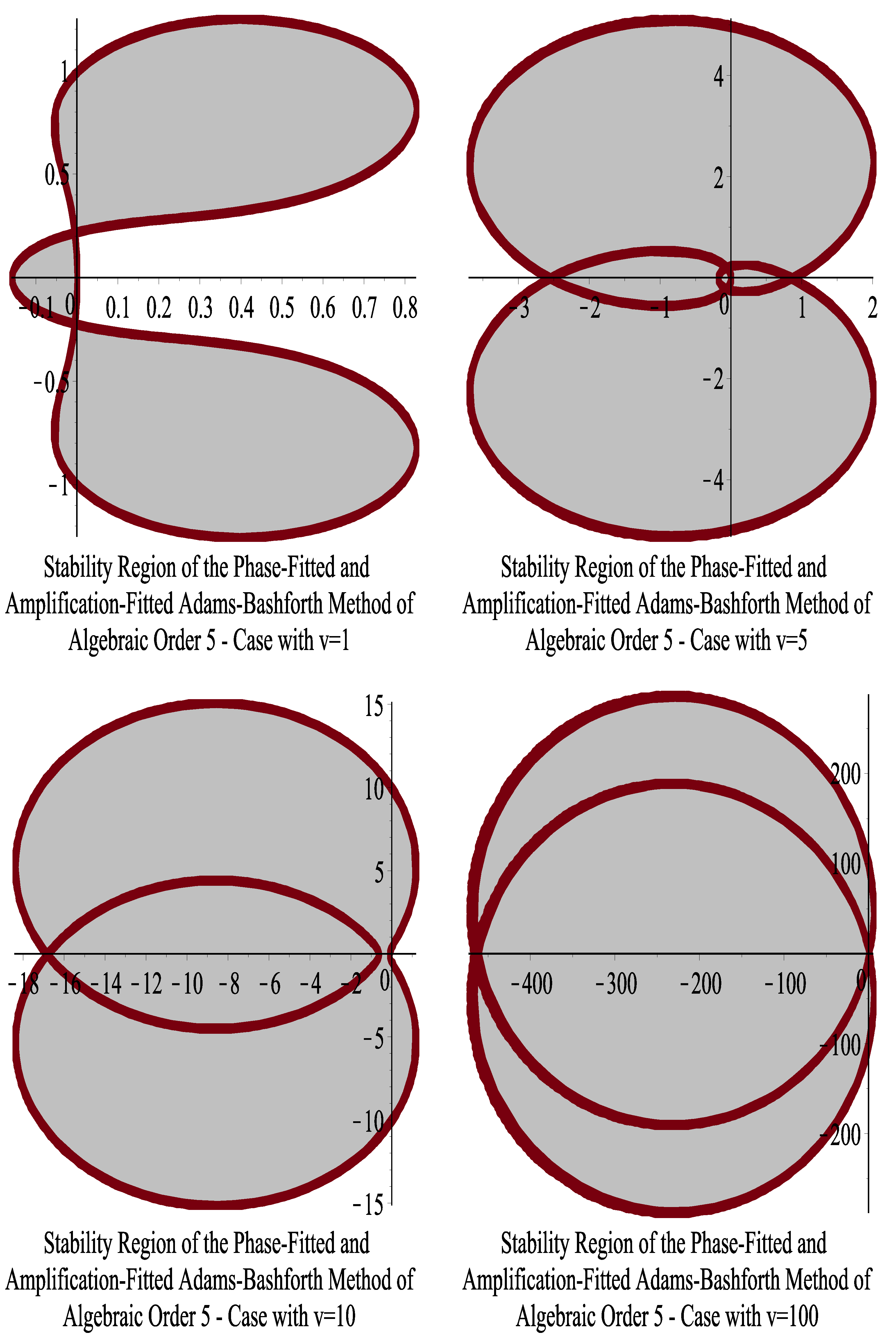
6. Phase-Fitted and Amplification-Fitted Adams–Bashforth Fifth-Order Method

We will investigate the following Adams–Bashforth approach:

$${\mathrm{\Phi }}_{n+1}-{\mathrm{\Phi }}_n=h\left({\mathrm{\Gamma }}_0\left(v\right){\mathrm{\Phi }}_n^{\prime }+{\mathrm{\Gamma }}_1\left(v\right){\mathrm{\Phi }}_{n-1}^{\prime }+{\mathrm{\Gamma }}_2\left(v\right){\mathrm{\Phi }}_{n-2}^{\prime }+{\mathrm{\Gamma }}_3{\mathrm{\Phi }}_{n-3}^{\prime }+{\displaystyle \frac{251}{720}}{\mathrm{\Phi }}_{n-4}^{\prime }\right),$$

(38)

which, for ${\mathrm{\Gamma }}_0\left(v\right)={\displaystyle \frac{1901}{720}}$, ${\mathrm{\Gamma }}_1\left(v\right)=-{\displaystyle \frac{2774}{720}}$, ${\mathrm{\Gamma }}_2\left(v\right)={\displaystyle \frac{2616}{720}}$ and ${\mathrm{\Gamma }}_3\left(v\right)=-{\displaystyle \frac{1274}{720}}$, achieves the fifth algebraic order:

$$LTE={\displaystyle \frac{95}{288}}{h}^6{\varphi }^{\left\{\left(6\right)\right\}}\left(t\right)+O\left(h^7\right),$$

(39)

where ($LTE$) is the local truncation error of the method.

Let us consider the method (38) with ${\mathrm{\Gamma }}_2\left(v\right)={\displaystyle \frac{2616}{720}}$ and ${\mathrm{\Gamma }}_3\left(v\right)=-{\displaystyle \frac{1274}{720}}$.

In order for the method (38) to be phase-fitted, the following relation must be true, according to the formula (17) that was described earlier:

$$PhErr={\displaystyle \frac{Pa{r}_9}{\frac{1261}{360}-4{\mathrm{\Gamma }}_0\left(v\right)-3{\mathrm{\Gamma }}_1\left(v\right)}}=0,$$

(40)

where

$$\begin{array}{ccc}\hfill Pa{r}_9& =& cos\left(5v\right)-cos\left(4v\right)+{\mathrm{\Gamma }}_0\left(v\right)vsin\left(4v\right)\hfill \\ & +& {\mathrm{\Gamma }}_1\left(v\right)vsin\left(3v\right)+{\displaystyle \frac{109}{30}}vsin\left(2v\right)-{\displaystyle \frac{637}{360}}vsin\left(v\right).\hfill \end{array}$$

(41)

Based on the formula (18) mentioned above, we know that in order for the method (38) to be amplification-fitted, the following relation must hold:

$$AF={\displaystyle \frac{Pa{r}_{10}}{-9v^2{\mathrm{\Gamma }}_1\left(v\right)-16v^2{\mathrm{\Gamma }}_0\left(v\right)-\frac{919v^2}{72}-1}}=0,$$

(42)

where

$$\begin{array}{ccc}\hfill Pa{r}_{10}& =& sin\left(5v\right)-sin\left(4v\right)-{\mathrm{\Gamma }}_0\left(v\right)vcos\left(4v\right)-{\mathrm{\Gamma }}_1\left(v\right)vcos\left(3v\right)\hfill \\ & -& {\displaystyle \frac{109}{30}}vcos\left(2v\right)+{\displaystyle \frac{637}{360}}vcos\left(v\right)-{\displaystyle \frac{251}{720}}v.\hfill \end{array}$$

(43)

Requesting the satisfaction of Equations (40) and (42), we obtain

$$\begin{array}{c}\hfill {\mathrm{\Gamma }}_0\left(v\right)={\displaystyle \frac{Pa{r}_{11}}{720vsin\left(v\right)}},\end{array}$$

(44)

$$\begin{array}{c}\hfill {\mathrm{\Gamma }}_1\left(v\right)=-{\displaystyle \frac{Pa{r}_{12}}{360vsin\left(v\right)}},\end{array}$$

(45)

where

$$\begin{array}{ccc}\hfill Pa{r}_{11}& =& 1004sin\left(v\right){\left(cos\left(v\right)\right)}^{2}v-2548sin\left(v\right)cos\left(v\right)v+2365vsin\left(v\right)\hfill \\ & -& 1440{\left(cos\left(v\right)\right)}^2+720cos\left(v\right)+720,\hfill \\ \hfill Pa{r}_{12}& =& 1004sin\left(v\right){\left(cos\left(v\right)\right)}^{3}v-2548sin\left(v\right){\left(cos\left(v\right)\right)}^{2}v+2114sin\left(v\right)cos\left(v\right)v\hfill \\ & +& 637vsin\left(v\right)-360cos\left(v\right)+360.\hfill \end{array}$$

(46)

                This novel algorithm has the following features:

$$\begin{array}{c}\hfill {\mathrm{\Gamma }}_0\left(v\right)\mathrm{is}\mathrm{given}\mathrm{by}\left(44\right)\\ \hfill {\mathrm{\Gamma }}_1\left(v\right)\mathrm{is}\mathrm{given}\mathrm{by}\left(45\right)\\ \hfill {\mathrm{\Gamma }}_2\left(v\right)={\displaystyle \frac{2616}{720}}\\ \hfill {\mathrm{\Gamma }}_3\left(v\right)=-{\displaystyle \frac{1274}{720}}\\ \hfill LTE={\displaystyle \frac{95}{288}}{h}^6\left({\mathrm{\Phi }}^{\left\{\left(6\right)\right\}}\left(t\right)-{\omega }^4{\mathrm{\Phi }}^{\left\{\left(2\right)\right\}}\left(t\right)\right)+O\left(h^7\right)\\ \hfill PhErr=0\\ \hfill AF=0,\end{array}$$

(47)

where $PhErr$ is the phase lag and $AF$ is the amplification factor.

The following are the formulae for the Taylor series expansion of the coefficients ${\mathrm{\Gamma }}_0\left(v\right)$ and ${\mathrm{\Gamma }}_1\left(v\right)$:

$$\begin{array}{ccc}\hfill {\mathrm{\Gamma }}_0\left(v\right)& =& {\displaystyle \frac{1901}{720}}+{\displaystyle \frac{95}{288}}{v}^4-{\displaystyle \frac{7001}{120960}}{v}^6+{\displaystyle \frac{3469}{806400}}{v}^8+\dots ,\hfill \\ \hfill {\mathrm{\Gamma }}_1\left(v\right)& =& -{\displaystyle \frac{1387}{360}}-{\displaystyle \frac{95}{288}}{v}^4+{\displaystyle \frac{1801}{4480}}{v}^6-{\displaystyle \frac{662077}{7257600}}{v}^8+\dots .\hfill \end{array}$$

(48)

7. Phase-Fitted and Amplification-Fitted Adams–Bashforth Fourth-Order Method with the Vanished First Derivative of the Phase Lag

We will investigate the Adams–Bashforth approach (38) with ${\mathrm{\Gamma }}_3\left(v\right)=-{\displaystyle \frac{1274}{720}}$.

Based on the formula (17) mentioned above, we know that in order for the method (38) to be phase-fitted, the following relation must hold:

$$PhErr={\displaystyle \frac{Pa{r}_{13}}{\frac{3877}{360}-4{\mathrm{\Gamma }}_0\left(v\right)-3{\mathrm{\Gamma }}_1\left(v\right)-2{\mathrm{\Gamma }}_2\left(v\right)}}=0,$$

(49)

where

$$\begin{array}{ccc}\hfill Pa{r}_{13}& =& cos\left(5v\right)-cos\left(4v\right)+{\mathrm{\Gamma }}_0\left(v\right)vsin\left(4v\right),\hfill \\ & +& {\mathrm{\Gamma }}_1\left(v\right)vsin\left(3v\right)+{\mathrm{\Gamma }}_2\left(v\right)vsin\left(2v\right)-{\displaystyle \frac{637vsin\left(v\right)}{360}}.\hfill \end{array}$$

(50)

Based on the formula (18) mentioned above, we know that in order for the method (38) to be amplification-fitted, the following relation must hold:

$$AF={\displaystyle \frac{Pa{r}_{14}}{-4v^2{\mathrm{\Gamma }}_2\left(v\right)-9v^2{\mathrm{\Gamma }}_1\left(v\right)-16v^2{\mathrm{\Gamma }}_0\left(v\right)+\frac{637v^2}{360}-1}}=0,$$

(51)

where

$$\begin{array}{ccc}\hfill Pa{r}_{14}& =& sin\left(5v\right)-sin\left(4v\right)-{\mathrm{\Gamma }}_0\left(v\right)vcos\left(4v\right),\hfill \\ & -& {\mathrm{\Gamma }}_1\left(v\right)vcos\left(3v\right)-{\mathrm{\Gamma }}_2\left(v\right)vcos\left(2v\right),\hfill \\ & +& {\displaystyle \frac{637vcos\left(v\right)}{360}}-{\displaystyle \frac{251v}{720}}.\hfill \end{array}$$

(52)

Applying the algorithm of Section 4 to the (38), we obtain that in order for the method (38) to have vanished the first derivative of the phase lag, the following relation must hold:

$${\displaystyle \frac{\partial PhErr}{\partial v}}={\displaystyle \frac{Pa{r}_{15}}{\frac{3877}{360}-4{\mathrm{\Gamma }}_0\left(v\right)-3{\mathrm{\Gamma }}_1\left(v\right)-2{\mathrm{\Gamma }}_2\left(v\right)}}=0,$$

(53)

where

$$\begin{array}{ccc}\hfill Pa{r}_{15}& =& -5sin\left(5v\right)+4sin\left(4v\right)+{\mathrm{\Gamma }}_0\left(v\right)sin\left(4v\right)\hfill \\ & +& 4{\mathrm{\Gamma }}_0\left(v\right)vcos\left(4v\right)+{\mathrm{\Gamma }}_1\left(v\right)sin\left(3v\right)+3{\mathrm{\Gamma }}_1\left(v\right)vcos\left(3v\right)\hfill \\ & +& {\mathrm{\Gamma }}_2\left(v\right)sin\left(2v\right)+2{\mathrm{\Gamma }}_2\left(v\right)vcos\left(2v\right)-{\displaystyle \frac{637sin\left(v\right)}{360}}-{\displaystyle \frac{637vcos\left(v\right)}{360}}.\hfill \end{array}$$

(54)

Requesting the satisfaction of Equations (49), (51) and (53), we obtain

$$\begin{array}{c}\hfill {\mathrm{\Gamma }}_0\left(v\right)={\displaystyle \frac{Pa{r}_{16}}{720v^{2}sin\left(v\right)\left(4{\left(cos\left(v\right)\right)}^3+4{\left(cos\left(v\right)\right)}^2-cos\left(v\right)-1\right)}},\end{array}$$

(55)

$$\begin{array}{c}\hfill {\mathrm{\Gamma }}_1\left(v\right)=-{\displaystyle \frac{Pa{r}_{17}}{360v^{2}sin\left(v\right)\left(4{\left(cos\left(v\right)\right)}^3+4{\left(cos\left(v\right)\right)}^2-cos\left(v\right)-1\right)}},\end{array}$$

(56)

$$\begin{array}{c}\hfill {\mathrm{\Gamma }}_2\left(v\right)=-{\displaystyle \frac{Pa{r}_{18}}{360v^{2}sin\left(v\right)\left(4{\left(cos\left(v\right)\right)}^3+4{\left(cos\left(v\right)\right)}^2-cos\left(v\right)-1\right)}},\end{array}$$

(57)

where the formulae $Pa{r}_{16}$, $Pa{r}_{17}$, and $Pa{r}_{18}$ are in Appendix C.

                This novel algorithm has the following features:

$$\begin{array}{c}\hfill {\mathrm{\Gamma }}_0\left(v\right)\mathrm{is}\mathrm{given}\mathrm{by}\left(55\right)\\ \hfill {\mathrm{\Gamma }}_1\left(v\right)\mathrm{is}\mathrm{given}\mathrm{by}\left(56\right)\\ \hfill {\mathrm{\Gamma }}_2\left(v\right)\mathrm{is}\mathrm{given}\mathrm{by}\left(57\right)\\ \hfill {\mathrm{\Gamma }}_3\left(v\right)=-{\displaystyle \frac{1274}{720}}\\ \hfill LTE={\displaystyle \frac{95}{432}}{h}^5\left({\omega }^2{\mathrm{\Phi }}^{\left\{\left(3\right)\right\}}\left(t\right)+{\omega }^4{\mathrm{\Phi }}^{\prime }\left(t\right)\right)+O\left(h^6\right)\\ \hfill PhErr=0\\ \hfill AF=0\\ \hfill DerPhErr=0,\end{array}$$

(58)

where $PhErr$ is the phase lag, $AF$ is the amplification factor, and $DerPhErr$ is the first derivative of the phase lag.

The following are the formulae for the Taylor series expansion of the coefficients ${\mathrm{\Gamma }}_0\left(v\right)$, ${\mathrm{\Gamma }}_1\left(v\right)$, and ${\mathrm{\Gamma }}_2\left(v\right)$:

$$\begin{array}{ccc}\hfill {\mathrm{\Gamma }}_0\left(v\right)& =& {\displaystyle \frac{1901}{720}}-{\displaystyle \frac{95v^2}{432}}+{\displaystyle \frac{41723v^4}{120960}}+{\displaystyle \frac{142499v^6}{518400}}+{\displaystyle \frac{356688701v^8}{1437004800}}+\dots ,\hfill \\ \hfill {\mathrm{\Gamma }}_1\left(v\right)& =& -{\displaystyle \frac{1387}{360}}+{\displaystyle \frac{95v^2}{216}}-{\displaystyle \frac{1299v^4}{2240}}-{\displaystyle \frac{417523v^6}{1814400}}-{\displaystyle \frac{178304297v^8}{718502400}}+\dots ,\hfill \\ \hfill {\mathrm{\Gamma }}_2\left(v\right)& =& {\displaystyle \frac{109}{30}}-{\displaystyle \frac{95v^2}{432}}+{\displaystyle \frac{1823v^4}{120960}}+{\displaystyle \frac{1207523v^6}{3628800}}+{\displaystyle \frac{350506943v^8}{1437004800}}+\dots .\hfill \end{array}$$

(59)

8. Phase-Fitted and Amplification-Fitted Adams–Bashforth Fifth-Order Method with the Vanished First Derivative of the Amplification Factor

We will investigate the Adams–Bashforth approach (38) with ${\mathrm{\Gamma }}_3\left(v\right)=-{\displaystyle \frac{1274}{720}}$.

Based on the formula (17) mentioned above, we know that in order for the method (38) to be phase-fitted, the relation (49) must hold.

Based on the formula (18) mentioned above, we know that in order for the method (38) to be amplification-fitted, the relation (51) must hold.

Applying the algorithm of Section 5 to (38), we obtain that in order for the method (38) to have vanished the first derivative of the amplification factor, the following relation must hold:

$${\displaystyle \frac{\partial AF}{\partial v}}=-{\displaystyle \frac{1}{2}}{\displaystyle \frac{Pa{r}_{19}}{{\left(5760v^2{\mathrm{\Gamma }}_0\left(v\right)+3240v^2{\mathrm{\Gamma }}_1\left(v\right)+1440v^2{\mathrm{\Gamma }}_2\left(v\right)-637v^2+360\right)}^2}}=0,$$

(60)

where $Pa{r}_{19}$ is given in Appendix D.

Requesting the satisfaction of Equations (49), (51), and (60), we obtain

$$\begin{array}{c}\hfill {\mathrm{\Gamma }}_0\left(v\right)={\displaystyle \frac{Pa{r}_{20}}{720sin\left(v\right)cos\left(v\right)v^2\left(4{\left(cos\left(v\right)\right)}^2-3\right)}},\end{array}$$

(61)

$$\begin{array}{c}\hfill {\mathrm{\Gamma }}_1\left(v\right)=-{\displaystyle \frac{Pa{r}_{21}}{360v^2\left(4{\left(cos\left(v\right)\right)}^2-3\right)sin\left(v\right)}},\end{array}$$

(62)

$$\begin{array}{c}\hfill {\mathrm{\Gamma }}_2\left(v\right)=-{\displaystyle \frac{Pa{r}_{22}}{360sin\left(v\right)cos\left(v\right)v^2\left(4{\left(cos\left(v\right)\right)}^2-3\right)}},\end{array}$$

(63)

where the formulae $Pa{r}_{20}$, $Pa{r}_{21}$, and $Pa{r}_{22}$ are in Appendix E.

               This novel algorithm has the following features:

$$\begin{array}{c}\hfill {\mathrm{\Gamma }}_0\left(v\right)\mathrm{is}\mathrm{given}\mathrm{by}\left(61\right)\\ \hfill {\mathrm{\Gamma }}_1\left(v\right)\mathrm{is}\mathrm{given}\mathrm{by}\left(62\right)\\ \hfill {\mathrm{\Gamma }}_2\left(v\right)\mathrm{is}\mathrm{given}\mathrm{by}\left(63\right)\\ \hfill {\mathrm{\Gamma }}_3\left(v\right)=-{\displaystyle \frac{1274}{720}}\\ \hfill LTE={\displaystyle \frac{95}{288}}{h}^6\left({\mathrm{\Phi }}^{\left\{\left(6\right)\right\}}\left(t\right)-{\omega }^4{\mathrm{\Phi }}^{\left\{\left(2\right)\right\}}\left(t\right)\right)+O\left(h^6\right)\\ \hfill PhErr=0\\ \hfill AF=0\\ \hfill DerAF=0,\end{array}$$

(64)

where $PhErr$ is the phase lag, $AF$ is the amplification factor, and $DerAF$ is the first derivative of the amplification factor.

The following are the formulae for the Taylor series expansion of the coefficients ${\mathrm{\Gamma }}_0\left(v\right)$, ${\mathrm{\Gamma }}_1\left(v\right)$, and ${\mathrm{\Gamma }}_2\left(v\right)$:

$$\begin{array}{ccc}\hfill {\mathrm{\Gamma }}_0\left(v\right)& =& {\displaystyle \frac{1901}{720}}+{\displaystyle \frac{32387v^4}{20160}}+{\displaystyle \frac{19867727v^6}{3628800}}+{\displaystyle \frac{9512718143v^8}{479001600}}+\dots ,\hfill \\ \hfill {\mathrm{\Gamma }}_1\left(v\right)& =& -{\displaystyle \frac{1387}{360}}-{\displaystyle \frac{14531v^4}{5040}}-{\displaystyle \frac{1216573v^6}{129600}}-{\displaystyle \frac{4116426883v^8}{119750400}}+\dots ,\hfill \\ \hfill {\mathrm{\Gamma }}_2\left(v\right)& =& {\displaystyle \frac{109}{30}}+{\displaystyle \frac{8579v^4}{6720}}+{\displaystyle \frac{2868251v^6}{518400}}+{\displaystyle \frac{9510657557v^8}{479001600}}+\dots .\hfill \end{array}$$

(65)

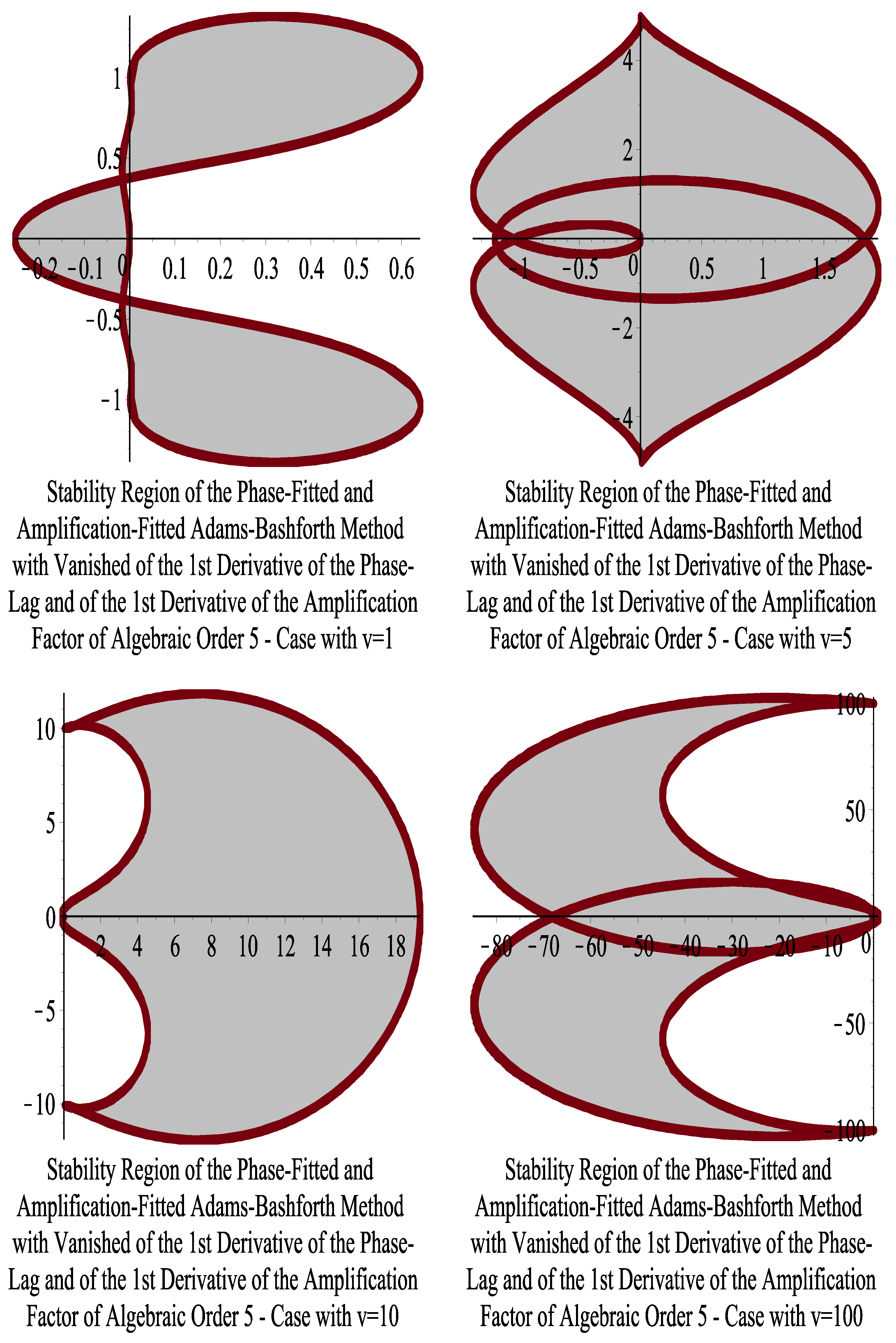
9. Phase-Fitted and Amplification-Fitted Adams–Bashforth Fifth-Order Method with the Vanished First Derivative of the Phase Lag and the First Derivative of the Amplification Factor

We will investigate the Adams–Bashforth approach (38).

Based on the formula (17) mentioned above, we know that in order for the method (38) to be phase-fitted, the following relation must hold:

$$PhErr={\displaystyle \frac{Pa{r}_{23}}{9-4{\mathrm{\Gamma }}_0\left(v\right)-3{\mathrm{\Gamma }}_1\left(v\right)-2{\mathrm{\Gamma }}_2\left(v\right)-{\mathrm{\Gamma }}_3\left(v\right)}},$$

(66)

where

$$\begin{array}{ccc}\hfill Pa{r}_{23}& =& cos\left(5v\right)-cos\left(4v\right)+{\mathrm{\Gamma }}_0\left(v\right)vsin\left(4v\right)\hfill \\ & +& {\mathrm{\Gamma }}_1\left(v\right)vsin\left(3v\right)+{\mathrm{\Gamma }}_2\left(v\right)vsin\left(2v\right)+{\mathrm{\Gamma }}_3\left(v\right)vsin\left(v\right)\hfill \end{array}$$

(67)

Based on the formula (18) mentioned above, we know that in order for the method (38) to be amplification-fitted, following relation must hold:

$$AF={\displaystyle \frac{Pa{r}_{24}}{-16v^2{\mathrm{\Gamma }}_0\left(v\right)-9v^2{\mathrm{\Gamma }}_1\left(v\right)-4v^2{\mathrm{\Gamma }}_2\left(v\right)-v^2{\mathrm{\Gamma }}_3\left(v\right)-1}},$$

(68)

where

$$\begin{array}{ccc}\hfill Pa{r}_{24}& =& sin\left(5v\right)-sin\left(4v\right)-{\mathrm{\Gamma }}_0\left(v\right)vcos\left(4v\right)-{\mathrm{\Gamma }}_1\left(v\right)vcos\left(3v\right)\hfill \\ & -& {\mathrm{\Gamma }}_2\left(v\right)vcos\left(2v\right)-{\mathrm{\Gamma }}_3\left(v\right)vcos\left(v\right)-{\displaystyle \frac{251v}{720}}.\hfill \end{array}$$

(69)

Applying the algorithm of Section 4 to the method (38), we obtain that in order for the method (38) to have vanished the first derivative of the phase lag, the following relation must hold:

$${\displaystyle \frac{\partial PhErr}{\partial v}}={\displaystyle \frac{Pa{r}_{30}}{9-4{\mathrm{\Gamma }}_0\left(v\right)-3{\mathrm{\Gamma }}_1\left(v\right)-2{\mathrm{\Gamma }}_2\left(v\right)-{\mathrm{\Gamma }}_3\left(v\right)}},$$

(70)

where

$$\begin{array}{ccc}\hfill Pa{r}_{30}& =& -5sin\left(5v\right)+4sin\left(4v\right)+{\mathrm{\Gamma }}_0\left(v\right)sin\left(4v\right)\hfill \\ & +& 4{\mathrm{\Gamma }}_0\left(v\right)vcos\left(4v\right)+{\mathrm{\Gamma }}_1\left(v\right)sin\left(3v\right)+3{\mathrm{\Gamma }}_1\left(v\right)vcos\left(3v\right)\hfill \\ & +& {\mathrm{\Gamma }}_2\left(v\right)sin\left(2v\right)+2{\mathrm{\Gamma }}_2\left(v\right)vcos\left(2v\right)\hfill \\ & +& {\mathrm{\Gamma }}_3\left(v\right)sin\left(v\right)+{\mathrm{\Gamma }}_3\left(v\right)vcos\left(v\right).\hfill \end{array}$$

(71)

Applying the algorithm of Section 5 to the method (38), we obtain that in order for the method (38) to have vanished the first derivative of the amplification factor, the following relation must hold:

$${\displaystyle \frac{\partial AF}{\partial v}}=-{\displaystyle \frac{Pa{r}_{31}}{720{\left(16v^2{\mathrm{\Gamma }}_0\left(v\right)+9v^2{\mathrm{\Gamma }}_1\left(v\right)+4v^2{\mathrm{\Gamma }}_2\left(v\right)+v^2{\mathrm{\Gamma }}_3\left(v\right)+1\right)}^2}}=0,$$

(72)

where $Pa{r}_{31}$ is given in Appendix F.

Requesting the satisfaction of Equations (66), (68), (70), and (72), we obtain

$$\begin{array}{c}\hfill {\mathrm{\Gamma }}_0\left(v\right)={\displaystyle \frac{Pa{r}_{32}}{720v^{2}sin\left(v\right)\left(cos\left(v\right)+1\right)}},\end{array}$$

(73)

$$\begin{array}{c}\hfill {\mathrm{\Gamma }}_1\left(v\right)=-{\displaystyle \frac{Pa{r}_{33}}{180v^{2}sin\left(v\right)\left(cos\left(v\right)+1\right)}},\end{array}$$

(74)

$$\begin{array}{c}\hfill {\mathrm{\Gamma }}_2\left(v\right)={\displaystyle \frac{Pa{r}_{34}}{360v^{2}sin\left(v\right)\left(cos\left(v\right)+1\right)}},\end{array}$$

(75)

$$\begin{array}{c}\hfill {\mathrm{\Gamma }}_3\left(v\right)=-{\displaystyle \frac{Pa{r}_{35}}{180v^{2}sin\left(v\right)\left(cos\left(v\right)+1\right)}},\end{array}$$

(76)

where the formulae $Pa{r}_{32}$, $Pa{r}_{33}$, $Pa{r}_{34}$, and $Pa{r}_{35}$ are in Appendix G.

                 This novel algorithm has the following features:

$$\begin{array}{c}\hfill {\mathrm{\Gamma }}_0\left(v\right)\mathrm{is}\mathrm{given}\mathrm{by}\left(73\right)\\ \hfill {\mathrm{\Gamma }}_1\left(v\right)\mathrm{is}\mathrm{given}\mathrm{by}\left(74\right)\\ \hfill {\mathrm{\Gamma }}_2\left(v\right)\mathrm{is}\mathrm{given}\mathrm{by}\left(75\right)\\ \hfill {\mathrm{\Gamma }}_3\left(v\right)\mathrm{is}\mathrm{given}\mathrm{by}\left(76\right)\\ \hfill LTE={\displaystyle \frac{95}{288}}{h}^6\left({\mathrm{\Phi }}^{\left\{\left(6\right)\right\}}\left(t\right)+2{\omega }^2{\mathrm{\Phi }}^{\left\{\left(4\right)\right\}}\left(t\right)+{\omega }^4{\mathrm{\Phi }}^{\left\{\left(2\right)\right\}}\left(t\right)\right)+O\left(h^6\right)\\ \hfill PhErr=0\\ \hfill AF=0\\ \hfill DerPhErr=0\\ \hfill DerAF=0,\end{array}$$

(77)

where $PhErr$ is the phase lag, $AF$ is the amplification factor, $DerPhErr$ is the first derivative of the phase lag, and $DerAF$ is the first derivative of the amplification factor.

The following are the formulae for the Taylor series expansion of the coefficients ${\mathrm{\Gamma }}_0\left(v\right)$, ${\mathrm{\Gamma }}_1\left(v\right)$, ${\mathrm{\Gamma }}_2\left(v\right)$, and ${\mathrm{\Gamma }}_3\left(v\right)$:

$$\begin{array}{ccc}\hfill {\mathrm{\Gamma }}_0\left(v\right)& =& {\displaystyle \frac{1901}{720}}-{\displaystyle \frac{95v^2}{144}}+{\displaystyle \frac{505v^4}{24192}}-{\displaystyle \frac{97v^6}{48384}}-{\displaystyle \frac{2953v^8}{19160064}}+\dots ,\hfill \\ \hfill {\mathrm{\Gamma }}_1\left(v\right)& =& -{\displaystyle \frac{1387}{360}}+{\displaystyle \frac{95v^2}{48}}-{\displaystyle \frac{17551v^4}{40320}}+{\displaystyle \frac{19361v^6}{518400}}-{\displaystyle \frac{1283617v^8}{479001600}}+\dots ,\hfill \\ \hfill {\mathrm{\Gamma }}_2\left(v\right)& =& {\displaystyle \frac{109}{30}}-{\displaystyle \frac{95v^2}{48}}+{\displaystyle \frac{19277v^4}{40320}}-{\displaystyle \frac{235789v^6}{3628800}}+{\displaystyle \frac{178207v^8}{43545600}}+\dots ,\hfill \\ \hfill {\mathrm{\Gamma }}_3\left(v\right)& =& -{\displaystyle \frac{637}{360}}+{\displaystyle \frac{95v^2}{144}}-{\displaystyle \frac{7703v^4}{120960}}+{\displaystyle \frac{3977v^6}{3628800}}-{\displaystyle \frac{24989v^8}{159667200}}.\hfill \end{array}$$

(78)

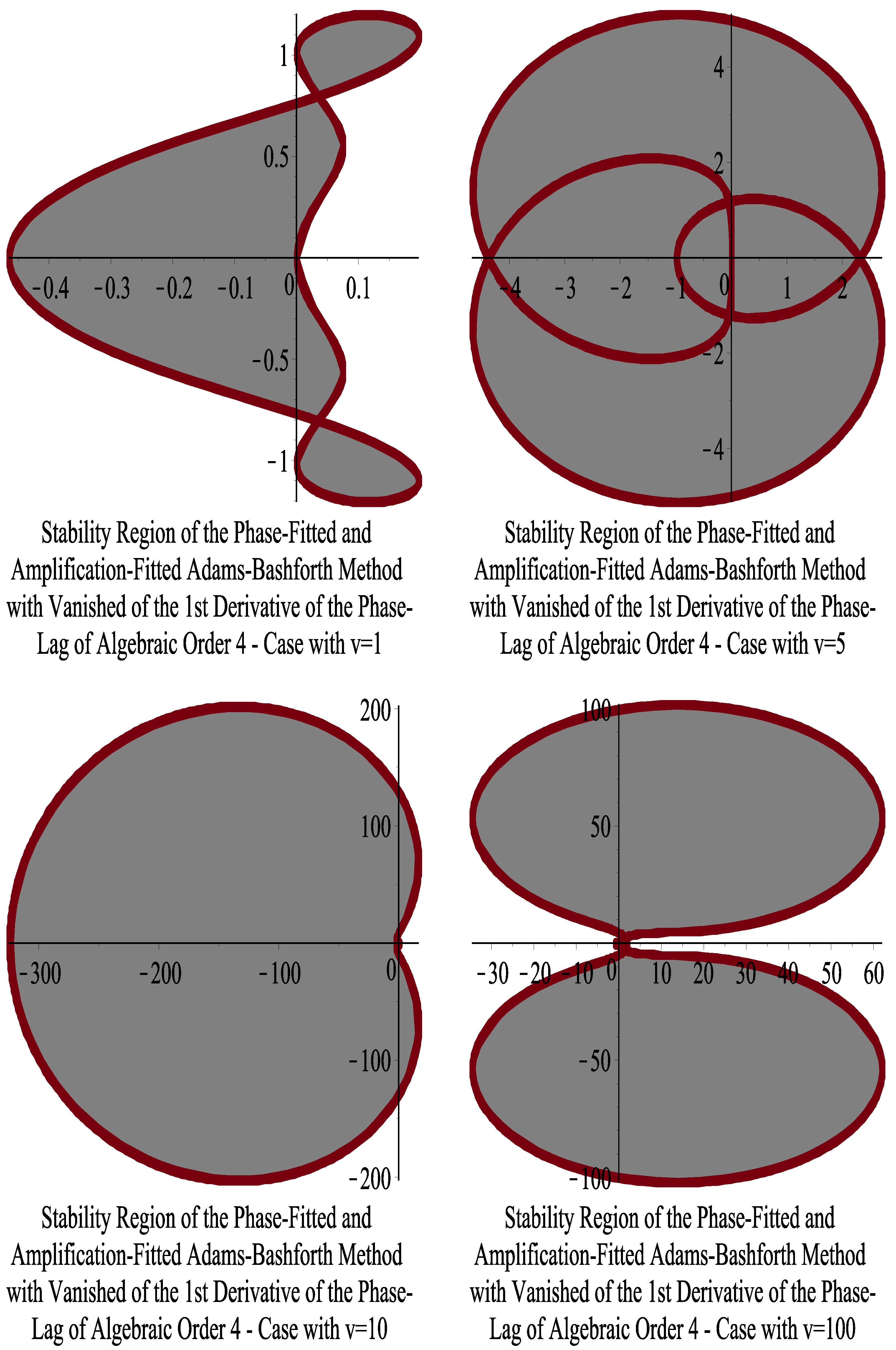
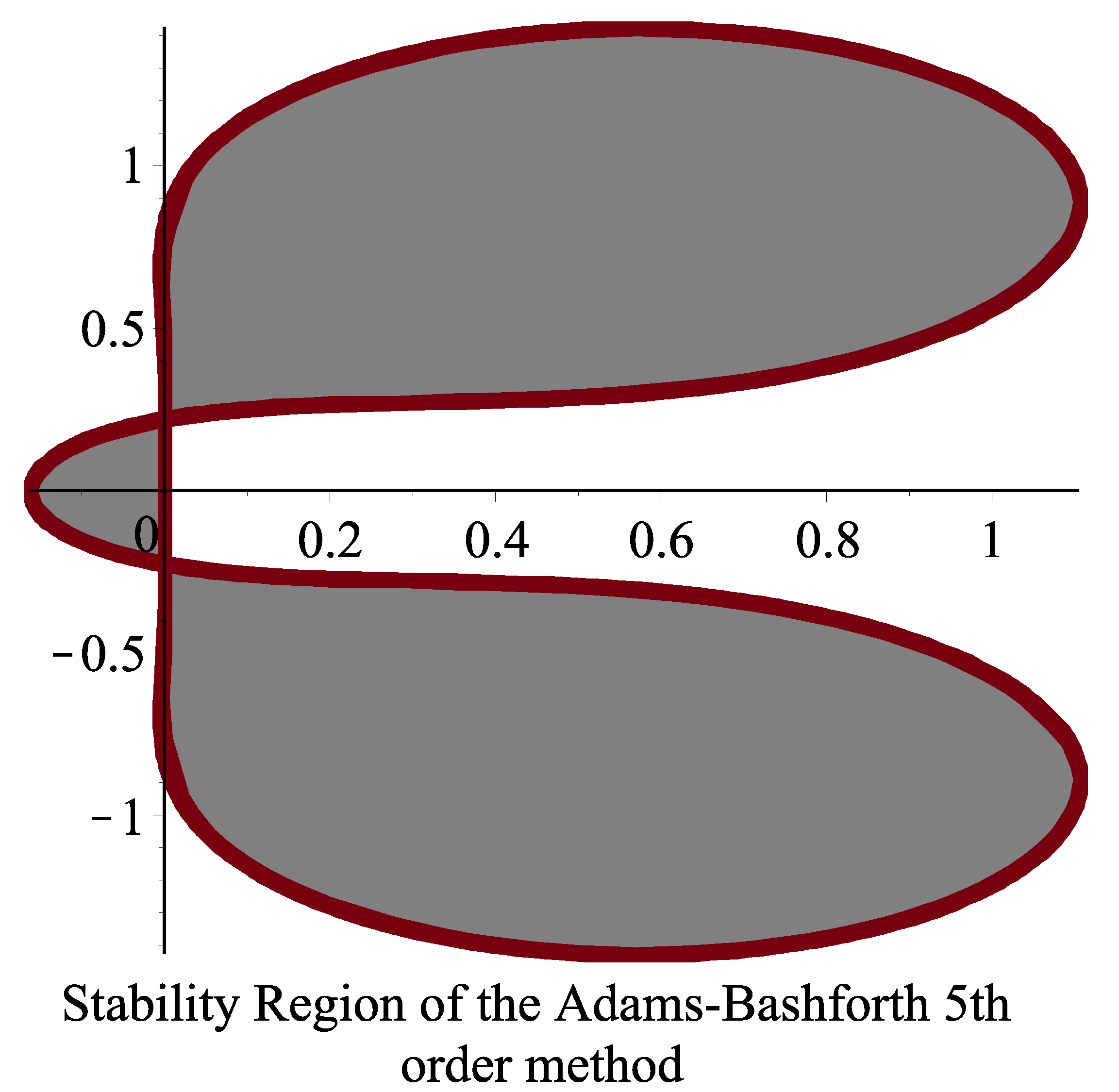
10. Stability Analysis

10.1. Five-Step Adams–Bashforth Methods

The five-step methods proposed by Adams–Bashforth are broadly described as follows:

$${\mathrm{\Phi }}_{n+1}-{\mathrm{\Phi }}_n=h\left(D_3{F}_n+D_2{F}_{n-1}+D_1{F}_{n-2}+D_0{F}_{n-3}\right),$$

(79)

where $F_{n+j}={\mathrm{\Phi }}_{n+j}^{\prime },j=-3\left(1\right)0$

The produced methods in Section 4 and Section 5, i.e., methods (29) and (36), belong to method (79).

Applying the scheme (79) to the scalar test equation

$${\mathrm{\Phi }}^{\prime }=\lambda \mathrm{\Phi }\mathrm{where}\lambda \in \mathcal{C},$$

(80)

we obtain the following difference equation

$${\mathrm{\Phi }}_{n+1}-{\mathrm{\Xi }}_3\left(V\right){\mathrm{\Phi }}_n-{\mathrm{\Xi }}_2\left(V\right){\mathrm{\Phi }}_{n-1}-{\mathrm{\Xi }}_1\left(V\right){\mathrm{\Phi }}_{n-2}-{\mathrm{\Xi }}_0\left(V\right){\mathrm{\Phi }}_{n-3}=0,$$

(81)

where $V=\lambda h$ and

$$\begin{array}{c}\hfill {\mathrm{\Xi }}_3\left(V\right)=1+D_{3}V,{\mathrm{\Xi }}_2\left(V\right)=D_{2}V,{\mathrm{\Xi }}_1\left(V\right)=D_{1}V,{\mathrm{\Xi }}_0\left(V\right)=D_{0}V.\end{array}$$

(82)

The characteristic equation of (81) is given by

$$q^4-{\mathrm{\Xi }}_3\left(V\right)q^3-{\mathrm{\Xi }}_2\left(V\right)q^2-{\mathrm{\Xi }}_1\left(V\right)q-{\mathrm{\Xi }}_0\left(V\right)=0.$$

(83)

If we solve the above equation using V and replace $i=\sqrt{-1}$ with $q=exp\left(i\zeta \right)$, we can draw the stability areas for $\zeta \in [0,2\pi ]$. Figure 1 and Figure 2 show the stability region for the algorithms obtained in Section 4 and Section 5. For these cases, we present the stability regions for $v=1$, $v=5$, $v=10$, and $v=100$.

10.2. Six-Step Adams–Bashforth Methods

The six-step methods proposed by Adams–Bashforth are broadly described as follows:

$${\mathrm{\Phi }}_{n+1}-{\mathrm{\Phi }}_n=h\left(E_4{F}_n+E_3{F}_{n-1}+E_2{F}_{n-2}+E_1{F}_{n-3}+E_0{F}_{n-4}\right),$$

(84)

where $F_{n+j}={\mathrm{\Phi }}_{n+j}^{\prime },j=-4\left(1\right)0$

The produced methods in Section 6, Section 7, Section 8 and Section 9, i.e., methods (47), (58), (64), and (77), belong to method (84).

Applying the scheme (84) to the scalar test Equation (80), we obtain the following difference equation:

$${\mathrm{\Phi }}_{n+1}-{\Delta }_4\left(V\right){\mathrm{\Phi }}_n-{\Delta }_3\left(V\right){\mathrm{\Phi }}_{n-1}-{\Delta }_2\left(V\right){\mathrm{\Phi }}_{n-2}-{\Delta }_1\left(V\right){\mathrm{\Phi }}_{n-3}-{\Delta }_0\left(V\right){\mathrm{\Phi }}_{n-4}=0,$$

(85)

where $V=\lambda h$ and

$$\begin{array}{c}\hfill {\Delta }_4\left(V\right)=1+E_{4}V,{\Delta }_3\left(V\right)=E_{3}V,{\Delta }_2\left(V\right)=E_{2}V,{\Delta }_1\left(V\right)=E_{1}V,{\Delta }_0\left(V\right)=E_{0}V.\end{array}$$

(86)

The characteristic equation of (85) is given by

$$q^5-{\Delta }_4\left(V\right)q^4-{\Delta }_3\left(V\right)q^3-{\Delta }_2\left(V\right)q^2-{\Delta }_1\left(V\right)q-{\Delta }_0\left(V\right)=0.$$

(87)

If we solve the above equation using V and replace $i=\sqrt{-1}$ with $q=exp\left(i\zeta \right)$, we can draw the stability areas for $\zeta \in [0,2\pi ]$. Figure 3 shows the stability of the six-step Adams–Bashforth method with constant coefficients. Figure 4, Figure 5, Figure 6 and Figure 7 show the stability region for the algorithms obtained in Section 6, Section 7, Section 8 and Section 9. For these cases, we present the stability regions for $v=1$, $v=5$, $v=10$, and $v=100$.

11. Numerical Results

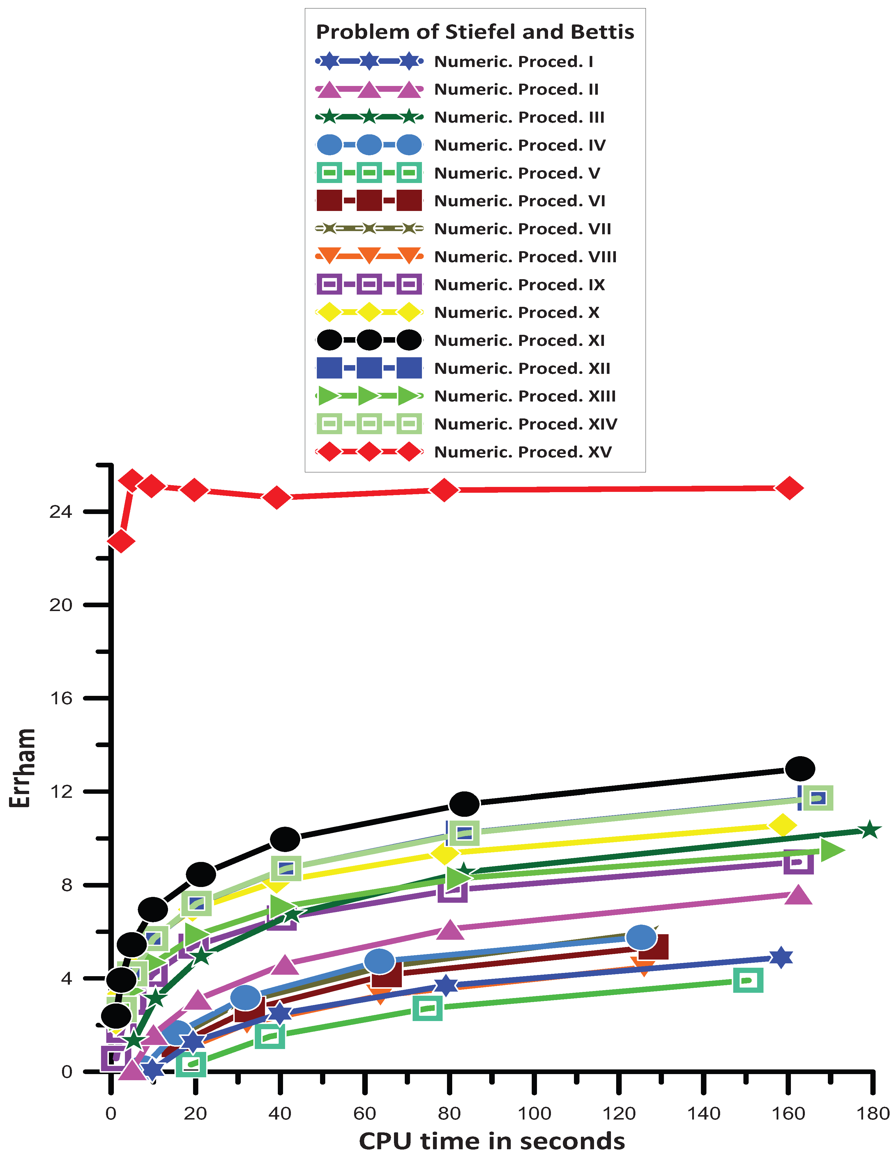
11.1. Problem of Stiefel and Bettis

Stiefel and Bettis [32] investigated the following nearly periodic orbit problem, which we take into consideration:

$$\begin{array}{ccc}\hfill {\mathrm{\Phi }}_1^{″}\left(t\right)& =& -{\mathrm{\Phi }}_1\left(t\right)+0.001cos\left(t\right),{\mathrm{\Phi }}_1\left(0\right)=1,{\mathrm{\Phi }}_1^{\prime }\left(0\right)=0,\hfill \\ \hfill {\mathrm{\Phi }}_2^{″}\left(t\right)& =& -{\mathrm{\Phi }}_2\left(t\right)+0.001sin\left(t\right),{\mathrm{\Phi }}_2\left(0\right)=0,{\mathrm{\Phi }}_2^{\prime }\left(0\right)=0.9995.\hfill \end{array}$$

(88)

The exact solution is

$$\begin{array}{c}\hfill {\mathrm{\Phi }}_1\left(t\right)=cos\left(t\right)+0.0005tsin\left(t\right),\\ \hfill {\mathrm{\Phi }}_2\left(t\right)=sin\left(t\right)-0.0005tcos\left(t\right).\end{array}$$

(89)

For this problem, we use $\omega =1$.

Numerical solutions to the problem (88) have been found for $0\le t\le 100,000$ using the respective methods:

• The classical Adams–Bashforth method of the fourth order, which is mentioned as Numeric. Proced. I;
• The classical Adams–Bashforth method of the fifth order, which is mentioned as Numeric. Proced. II;
• The classical Adams–Bashforth method of the sixth order, which is mentioned as Numeric. Proced. III;
• The Runge–Kutta Dormand and Prince fourth-order method [16], which is mentioned as Numeric. Proced. IV;
• The Runge–Kutta Dormand and Prince fifth order method [16], which is mentioned as Numeric. Proced. V
• The Runge–Kutta Fehlberg fourth-order method [33], which is mentioned as Numeric. Proced. VI;
• The Runge–Kutta Fehlberg fifth-order method [33], which is mentioned as Numeric. Proced. VII;
• The Runge–Kutta Cash and Karp fifth-order method [34], which is mentioned as Numeric. Proced. VIII;
• The phase-fitted and amplification-fitted Adams–Bashforth fourth-order method, which is developed in Section 8 of [30], which is mentioned as Numeric. Proced. IX;
• The phase-fitted and amplification-fitted Adams–Bashforth fourth-order method with the vanished first derivative of the phase lag which is developed in Section 4, which is mentioned as Numeric. Proced. X;
• The phase-fitted and amplification-fitted Adams–Bashforth fourth-order method with the vanished first derivative of the amplification factor, which is developed in Section 5, which is mentioned as Numeric. Proced. XI;
• The phase-fitted and amplification-fitted Adams–Bashforth fifth-order method which is developed in Section 6, which is mentioned as Numeric. Proced. XII;
• The phase-fitted and amplification-fitted Adams–Bashforth fifth-order method with the vanished first derivative of the phase lag which is developed in Section 7, which is mentioned as Numeric. Proced. XIII;
• The phase-fitted and amplification-fitted Adams–Bashforth fifth-order method with the vanished first derivative of the amplification factor which is developed in Section 8, which is mentioned as Numeric. Proced. XIV;
• The phase-fitted and amplification-fitted Adams–Bashforth fifth-order method with vanished the first derivative of the phase lag and the vanished first derivative of the amplification factor which is developed in Section 9, which is mentioned as Numeric. Proced. XV.

The highest absolute error of the solution obtained by each of the numerical approaches outlined earlier for the Stiefel and Bettis [32] problem is shown in Figure 8.

The information in Figure 8 allows us to see the following:

• Numeric. Proced. I is more efficient than Numeric. Proced. V;
• Numeric. Proced. I and Numeric. Proced. VIII give approximately the same accuracy;
• Numeric. Proced. VI is more efficient than Numeric. Proced. I;
• Numeric. Proced. IV is more efficient than Numeric. Proced. VI;
• Numeric. Proced. IV and Numeric. Proced. VII give approximately the same accuracy;
• Numeric. Proced. II is more efficient than Numeric. Proced. IV;
• Numeric. Proced. III is more efficient than Numeric. Proced. II;
• Numeric. Proced. IX gives mixed results. For big step sizes, it is more efficient than Numeric. Proced. III. For small step sizes, it is less efficient than Numeric. Proced. III;
• Numeric. Proced. XIII is more efficient than Numeric. Proced. IX;
• Numeric. Proced. X is more efficient than Numeric. Proced. XIII;
• Numeric. Proced. XIV is more efficient than Numeric. Proced. X;
• Numeric. Proced. XII and Numeric. Proced. XIV give approximately the same accuracy;
• Numeric. Proced. XI is more efficient than Numeric. Proced. XIV;
• Finally, Numeric. Proced. XV is the most efficient one.

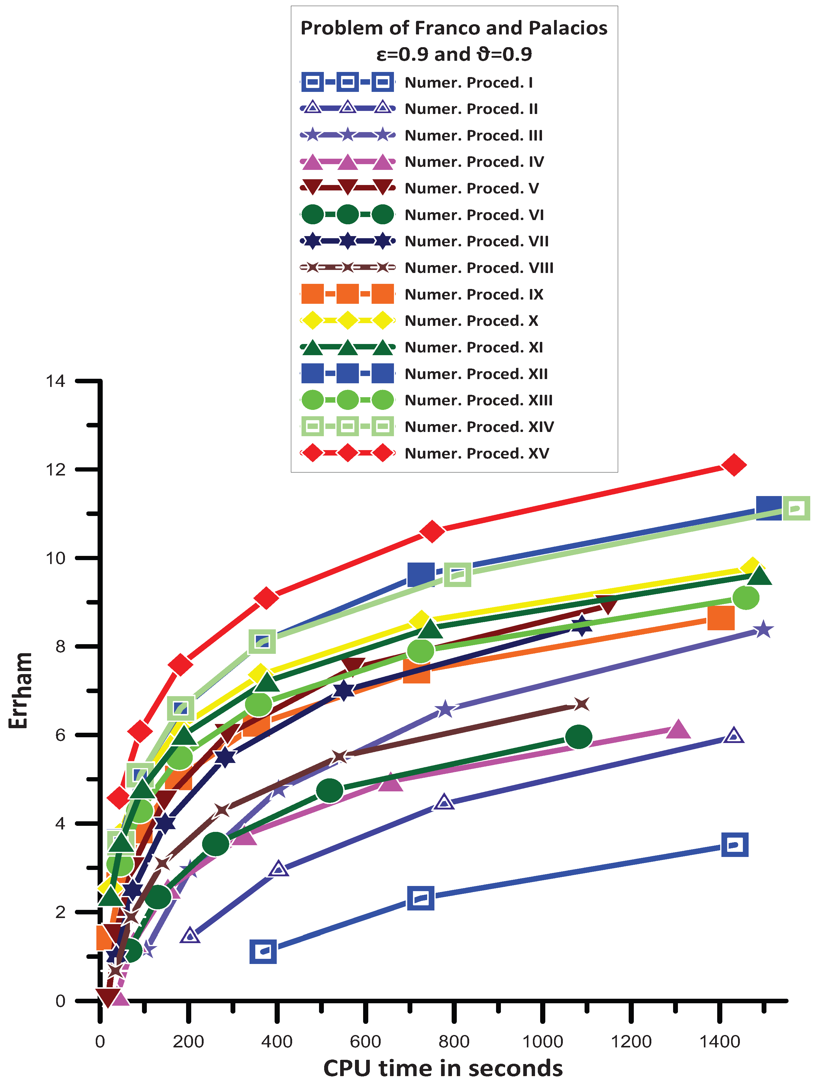
11.2. Problem of Franco and Palacios [35]

Franco and Palacios [35] investigated the following problem, which we take into consideration:

$$\begin{array}{ccc}\hfill {\mathrm{\Phi }}_1^{″}\left(t\right)& =& -{\mathrm{\Phi }}_1\left(t\right)+\epsilon cos\left(\vartheta t\right),{\mathrm{\Phi }}_1\left(0\right)=1,{\mathrm{\Phi }}_1^{\prime }\left(0\right)=0,\hfill \\ \hfill {\mathrm{\Phi }}_2^{″}\left(t\right)& =& -{\mathrm{\Phi }}_2\left(t\right)+\epsilon sin\left(\vartheta t\right),{\mathrm{\Phi }}_2\left(0\right)=0,{\mathrm{\Phi }}_2^{\prime }\left(0\right)=1.\hfill \end{array}$$

(90)

The exact solution is

$$\begin{array}{c}\hfill {\mathrm{\Phi }}_1\left(t\right)={\displaystyle \frac{1-\epsilon -{\vartheta }^2}{1-{\vartheta }^2}}cos\left(t\right)+{\displaystyle \frac{\epsilon }{1-{\vartheta }^2}}cos\left(\vartheta t\right),\\ \hfill {\mathrm{\Phi }}_2\left(t\right)={\displaystyle \frac{1-\epsilon \vartheta -{\vartheta }^2}{1-{\vartheta }^2}}sin\left(t\right)+{\displaystyle \frac{\epsilon }{1-{\vartheta }^2}}sin\left(\vartheta t\right),\end{array}$$

(91)

where $\epsilon =0.9$ and $\vartheta =0.9$. For this problem, we use $\omega =max\left(1,\left|\vartheta \right|\right)$.

Using the techniques outlined in Section 11.1, the numerical solution to the system of Equations (90) has been found for $0\le t\le 1,000,000$.

The information in Figure 9 allows us to see the following:

• Numeric. Proced. II is more efficient than Numeric. Proced. I;
• Numeric. Proced. IV is more efficient than Numeric. Proced. II;
• Numeric. Proced. IV and Numeric. Proced. VI give approximately the same accuracy;
• Numeric. Proced. III is more efficient than Numeric. Proced. IV;
• Numeric. Proced. VIII gives mixed results. For big step sizes, it is more efficient than Numeric. Proced. III. For small step sizes, it is less efficient than Numeric. Proced. III;
• Numeric. Proced. VII is more efficient than Numeric. Proced. III and Numeric. Proced. VIII;
• Numeric. Proced. XIII is more efficient than Numeric. Proced. VII;
• Numeric. Proced. IX gives mixed results. For big step sizes, it is more efficient than Numeric. Proced. VII. For small step sizes, it is less efficient than Numeric. Proced. VII;
• Numeric. Proced. V is more efficient than Numeric. Proced. IX;
• Numeric. Proced. XI is more efficient than Numeric. Proced. V;
• Numeric. Proced. X is more efficient than Numeric. Proced. XI;
• Numeric. Proced. XIV is more efficient than Numeric. Proced. X;
• Numeric. Proced. XII and Numeric. Proced. XIV give approximately the same accuracy;
• Finally, Numeric. Proced. XV is the most efficient one.

11.3. Nonlinear Problem of Petzold [36]

Petzold [36] investigated the following problem, which we take into consideration:

$$\begin{array}{c}\hfill {\mathrm{\Phi }}_1^{\prime }\left(t\right)=\lambda {\mathrm{\Phi }}_2\left(t\right),{\mathrm{\Phi }}_1\left(0\right)=1,\\ \hfill {\mathrm{\Phi }}_2^{\prime }\left(t\right)=-\lambda {\mathrm{\Phi }}_1\left(t\right)+{\displaystyle \frac{\alpha }{\lambda }}sin\left(\lambda x\right),{\mathrm{\Phi }}_2\left(0\right)=-{\displaystyle \frac{\alpha }{2{\lambda }^2}}.\end{array}$$

(92)

The exact solution is

$$\begin{array}{c}\hfill {\mathrm{\Phi }}_1\left(t\right)=\left(1-{\displaystyle \frac{\alpha }{2\lambda }}t\right)cos\left(\lambda t\right),\\ \hfill {\mathrm{\Phi }}_2\left(t\right)=-\left(1-{\displaystyle \frac{\alpha }{2\lambda }}t\right)sin\left(\lambda t\right)-{\displaystyle \frac{\alpha }{2{\lambda }^2}}cos\left(\lambda x\right),\end{array}$$

(93)

where $\lambda =1000$, $\alpha =100$. For this problem, we use $\omega =1000$.

Using the techniques outlined in Section 11.1, the numerical solution to the system of Equation (92) has been found for $0\le t\le 1000$.

The information in Figure 10 allows us to see the following:

• Numeric. Proced. I, Numeric. Proced. V and Numeric. Proced. VI give approximately the same accuracy;
• Numeric. Proced. VIII is more efficient than Numeric. Proced. VI;
• Numeric. Proced. VII is more efficient than Numeric. Proced. VIII;
• Numeric. Proced. II, Numeric. Proced. IV, and Numeric. Proced. VII give approximately the same accuracy;
• Numeric. Proced. III is more efficient than Numeric. Proced. II;
• Numeric. Proced. IX is more efficient than Numeric. Proced. III;
• Numeric. Proced. XIII is more efficient than Numeric. Proced. IX;
• Numeric. Proced. X is more efficient than Numeric. Proced. XIII;
• Numeric. Proced. XII is more efficient than Numeric. Proced. X;
• Numeric. Proced. XII and Numeric. Proced. XIV give approximately the same accuracy;
• Numeric. Proced. XI is more efficient than Numeric. Proced. XIV;
• Finally, Numeric. Proced. XV is the most efficient one.

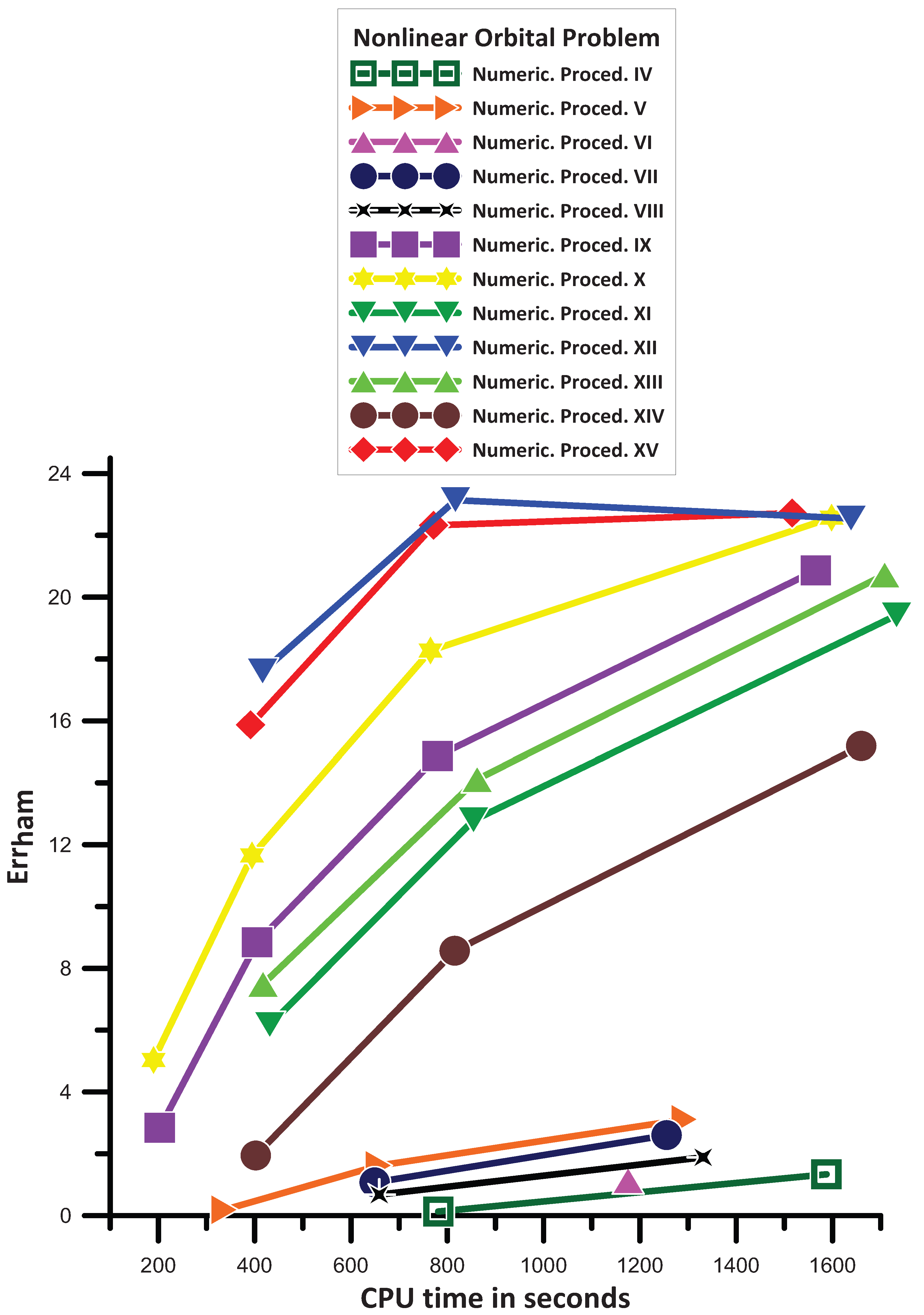
11.4. A Nonlinear Orbital Problem [37]

Simos in [37] investigated the following nonlinear orbital problem, which we take into consideration:

$$\begin{array}{ccc}\hfill {\mathrm{\Phi }}_1^{″}\left(t\right)& =& -{\phi }^2{\mathrm{\Phi }}_1\left(t\right)+{\displaystyle \frac{2{\mathrm{\Phi }}_1\left(t\right){\mathrm{\Phi }}_2\left(t\right)-sin\left(2\phi t\right)}{{\left({\mathrm{\Phi }}_1{\left(t\right)}^2+{\mathrm{\Phi }}_2{\left(t\right)}^2\right)}^{\frac{3}{2}}}},{\mathrm{\Phi }}_1\left(0\right)=1,{\mathrm{\Phi }}_1^{\prime }\left(0\right)=0,\hfill \\ \hfill {\mathrm{\Phi }}_2^{″}\left(t\right)& =& -{\phi }^2{\mathrm{\Phi }}_2\left(t\right)+{\displaystyle \frac{{\mathrm{\Phi }}_1{\left(t\right)}^2-{\mathrm{\Phi }}_2{\left(t\right)}^2-cos\left(2\phi t\right)}{{\left({\mathrm{\Phi }}_1{\left(t\right)}^2+{\mathrm{\Phi }}_2{\left(t\right)}^2\right)}^{\frac{3}{2}}}},{\mathrm{\Phi }}_2\left(0\right)=0,{\mathrm{\Phi }}_2^{\prime }\left(0\right)=\phi .\hfill \end{array}$$

(94)

The exact solution is

$${\mathrm{\Phi }}_1\left(t\right)=cos\left(\phi t\right),{\mathrm{\Phi }}_2\left(t\right)=sin\left(\phi t\right).$$

(95)

where $\phi =100$. For this problem, we use $\omega =100$.

Using the techniques outlined in Section 11.1, the numerical solution to the system of Equations (92) has been found for $0\le t\le 100,000$.

The information in Figure 11 allows us to see the following:

• Numeric. Proced. I, Numeric. Proced. II, and Numeric. Proced. III are divergent for the data of the specific problem;
• Numeric. Proced. VI gives the same accuracy as Numeric. Proced. IV in the one point of its convergence;
• Numeric. Proced. VIII is more efficient than Numeric. Proced. IV;
• Numeric. Proced. VII is more efficient than Numeric. Proced. VIII;
• Numeric. Proced. V is more efficient than Numeric. Proced. VII;
• Numeric. Proced. XIV is more efficient than Numeric. Proced. V;
• Numeric. Proced. XI is more efficient than Numeric. Proced. XIV;
• Numeric. Proced. XIII is more efficient than Numeric. Proced. XI;
• Numeric. Proced. IX is more efficient than Numeric. Proced. XIII;
• Numeric. Proced. X is more efficient than Numeric. Proced. IX;
• Numeric. Proced. XV and Numeric. Proced. XII give approximately the same accuracy;
• Finally, Numeric. Proced. XV and Numeric. Proced. XII are the most efficient.

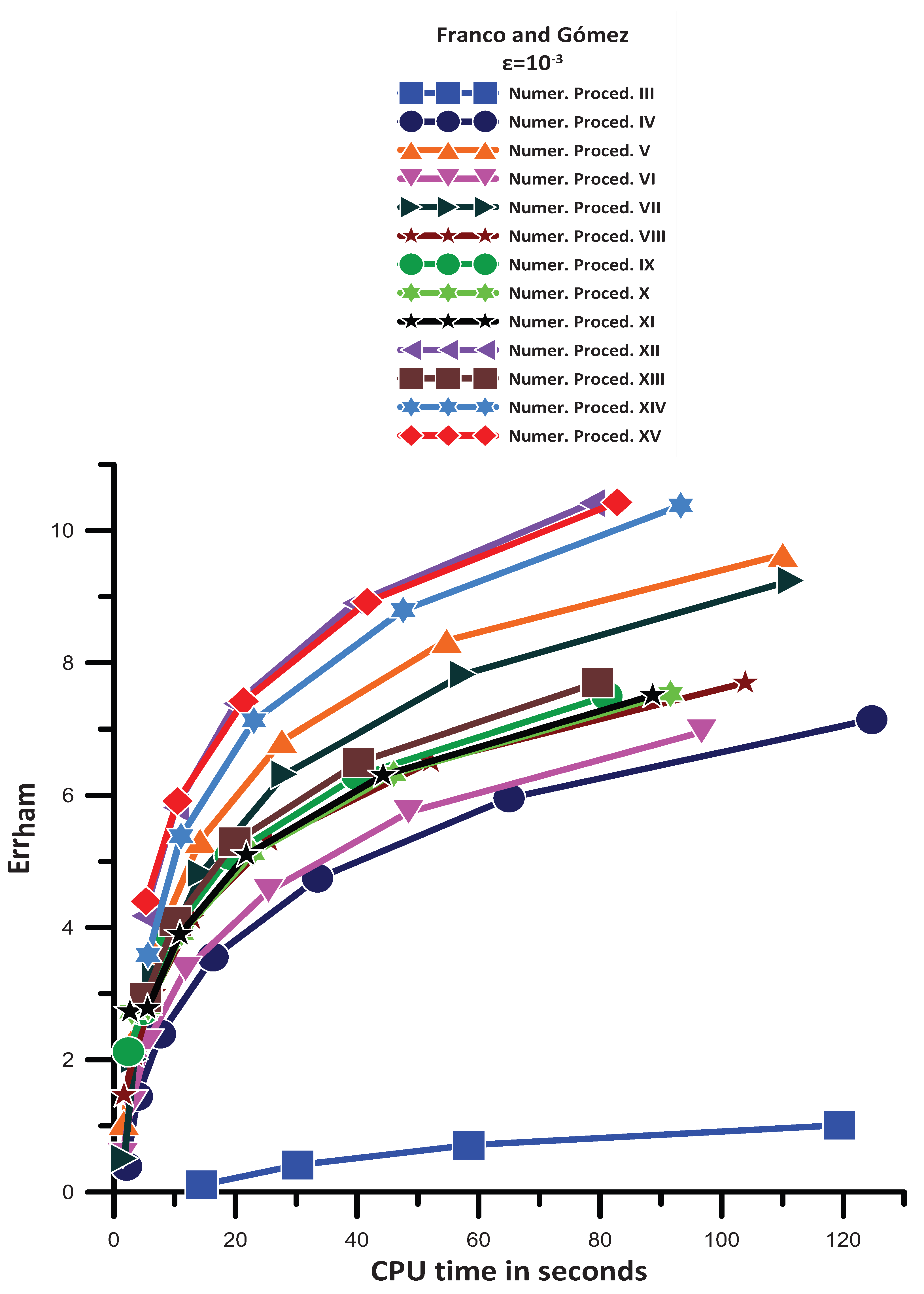
11.5. Problem of Franco and Gómez [38]

Franco and Gómez [38] investigated the following problem, which we take into consideration:

$$\begin{array}{ccc}\hfill {\mathrm{\Phi }}_1^{″}\left(t\right)& =& -199{\mathrm{\Phi }}_1\left(t\right)-198{\mathrm{\Phi }}_2\left(t\right)+{\left({\mathrm{\Phi }}_1\left(t\right)+{\mathrm{\Phi }}_2\left(t\right)\right)}^2+{sin}^2\left(10t\right)-1,\hfill \\ \hfill {\mathrm{\Phi }}_1\left(0\right)& =& 2,{\mathrm{\Phi }}_1^{\prime }\left(0\right)=-\epsilon ,\hfill \\ \hfill {\mathrm{\Phi }}_2^{″}\left(t\right)& =& 99{\mathrm{\Phi }}_1\left(t\right)+98{\mathrm{\Phi }}_2\left(t\right)+{\left({\mathrm{\Phi }}_1\left(t\right)+2{\mathrm{\Phi }}_2\left(t\right)\right)}^2+{\epsilon }^2{cos}^2\left(t\right)-{\epsilon }^2,\hfill \\ \hfill {\mathrm{\Phi }}_2\left(0\right)& =& -1,{\mathrm{\Phi }}_2^{\prime }\left(0\right)=\epsilon .\hfill \end{array}$$

(96)

The exact solution is

$$\begin{array}{c}\hfill {\mathrm{\Phi }}_1\left(t\right)=2cos\left(10t\right)-\epsilon sin\left(t\right),\\ \hfill {\mathrm{\Phi }}_2\left(t\right)=-cos\left(10t\right)+\epsilon sin\left(t\right).\end{array}$$

(97)

where $\epsilon ={10}^{-3}$. For this problem, we use $\omega =max\left(1,\left|\vartheta \right|\right)$.

Using the techniques outlined in Section 11.1, the numerical solution to the system of Equations (90) has been found for $0\le t\le 1,000,000$.

The information in Figure 12 allows us to see the following:

• Numeric. Proced. I and Numeric. Proced. II are divergent in the data of the specific problem;
• Numeric. Proced. IV is more efficient than Numeric. Proced. III;
• Numeric. Proced. VI is more efficient than Numeric. Proced. IV;
• Numeric. Proced. VIII is more efficient than Numeric. Proced. VI;
• Numeric. Proced. VIII, Numeric. Proced. X, and Numeric. Proced. XI give approximately the same accuracy;
• Numeric. Proced. IX is more efficient than Numeric. Proced. XI;
• Numeric. Proced. XIII is more efficient than Numeric. Proced. IX;
• Numeric. Proced. VII is more efficient than Numeric. Proced. XIII;
• Numeric. Proced. V is more efficient than Numeric. Proced. VII;
• Numeric. Proced. XIV is more efficient than Numeric. Proced. V;
• Numeric. Proced. XV is more efficient than Numeric. Proced. XIV;
• Numeric. Proced. XII and Numeric. Proced. XV give approximately the same accuracy, and they are the most efficient.

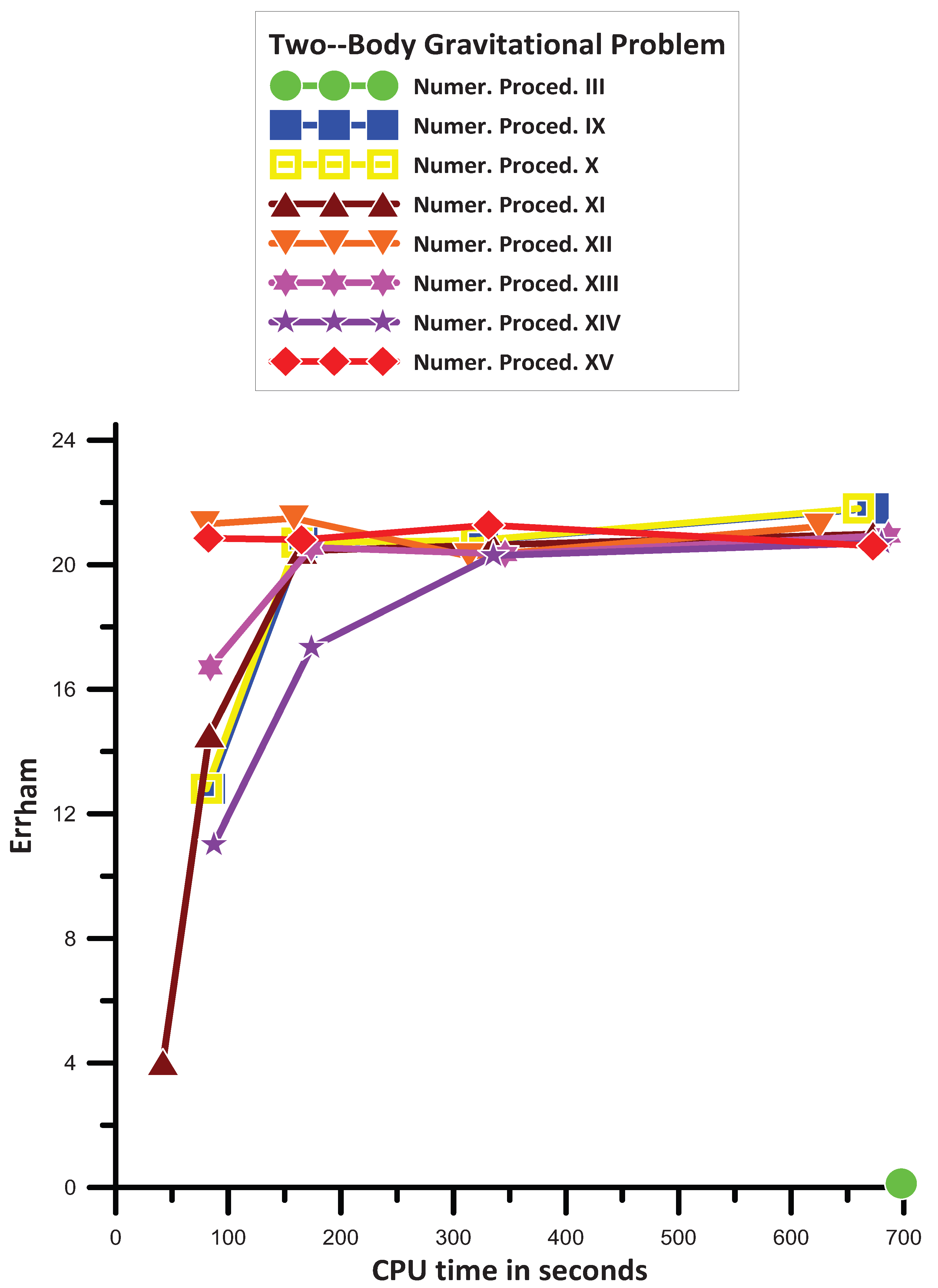
11.6. Two-Body Gravitational Problem

We take into consideration the two-body gravitational problem

$$\begin{array}{c}\hfill {\mathrm{\Phi }}_1^{″}\left(x\right)=-{\displaystyle \frac{{\mathrm{\Phi }}_1\left(x\right)}{{\left({\mathrm{\Phi }}_1{\left(x\right)}^2+{\mathrm{\Phi }}_2{\left(x\right)}^2\right)}^{\frac{3}{2}}}},{\mathrm{\Phi }}_1\left(0\right)=1,{\mathrm{\Phi }}_1^{\prime }\left(0\right)=0,\\ \hfill {\mathrm{\Phi }}_2^{″}\left(x\right)=-{\displaystyle \frac{{\mathrm{\Phi }}_2\left(x\right)}{{\left({\mathrm{\Phi }}_1{\left(x\right)}^2+{\mathrm{\Phi }}_2{\left(x\right)}^2\right)}^{\frac{3}{2}}}},{\mathrm{\Phi }}_2\left(0\right)=0,{\mathrm{\Phi }}_2^{\prime }\left(0\right)=1.\end{array}$$

(98)

The exact solution is

$$\begin{array}{c}\hfill {\mathrm{\Phi }}_1\left(x\right)=cos\left(x\right),\\ \hfill {\mathrm{\Phi }}_2\left(x\right)=sin\left(x\right).\end{array}$$

(99)

For this problem, we use $\omega ={\displaystyle \frac{1}{{\left({\mathrm{\Phi }}_1{\left(x\right)}^2+{\mathrm{\Phi }}_2{\left(x\right)}^2\right)}^{\frac{3}{4}}}}$.

Using the techniques outlined in Section 11.1, the numerical solution to the system of Equations (98) has been found for $0\le t\le 1,000,000$.

The information in Figure 13 allows us to see the following:

• Numeric. Proced. I, Numeric. Proced. II, Numeric. Proced. IV, Numeric. Proced. V, Numeric. Proced. VI, Numeric. Proced. VII, and Numeric. Proced. VIII are divergent in the data of the specific problem.
• Numeric. Proced. III is convergent but gives one result of low accuracy.
• Numeric. Proced. IX, Numeric. Proced. X, Numeric. Proced. XI, Numeric. Proced. XII, Numeric. Proced. XIII, Numeric. Proced. XIV, and Numeric. Proced. XV give approximately the same accuracy for small step sizes. The accuracy given by the above methods is high.
• For large step sizes, we have the following remarks:

  -

  Numeric. Proced. IX and Numeric. Proced. X are more efficient than Numeric. Proced. XIV;

  -

  Numeric. Proced. XI is more efficient than Numeric. Proced. IX and Numeric. Proced. X;

  -

  Numeric. Proced. XIII is more efficient than Numeric. Proced. XI;

  -

  Numeric. Proced. XV is more efficient than Numeric. Proced. XIII;

  -

  Numeric. Proced. XII is more efficient than Numeric. Proced. XV.

• Based on the above, Numeric. Proced. IX, Numeric. Proced. X, Numeric. Proced. XI, Numeric. Proced. XII, Numeric. Proced. XIII, Numeric. Proced. XIV, and Numeric. Proced. XV are the most efficient for small step sizes. For large step sizes Numeric. Proced. XII is the most efficient.

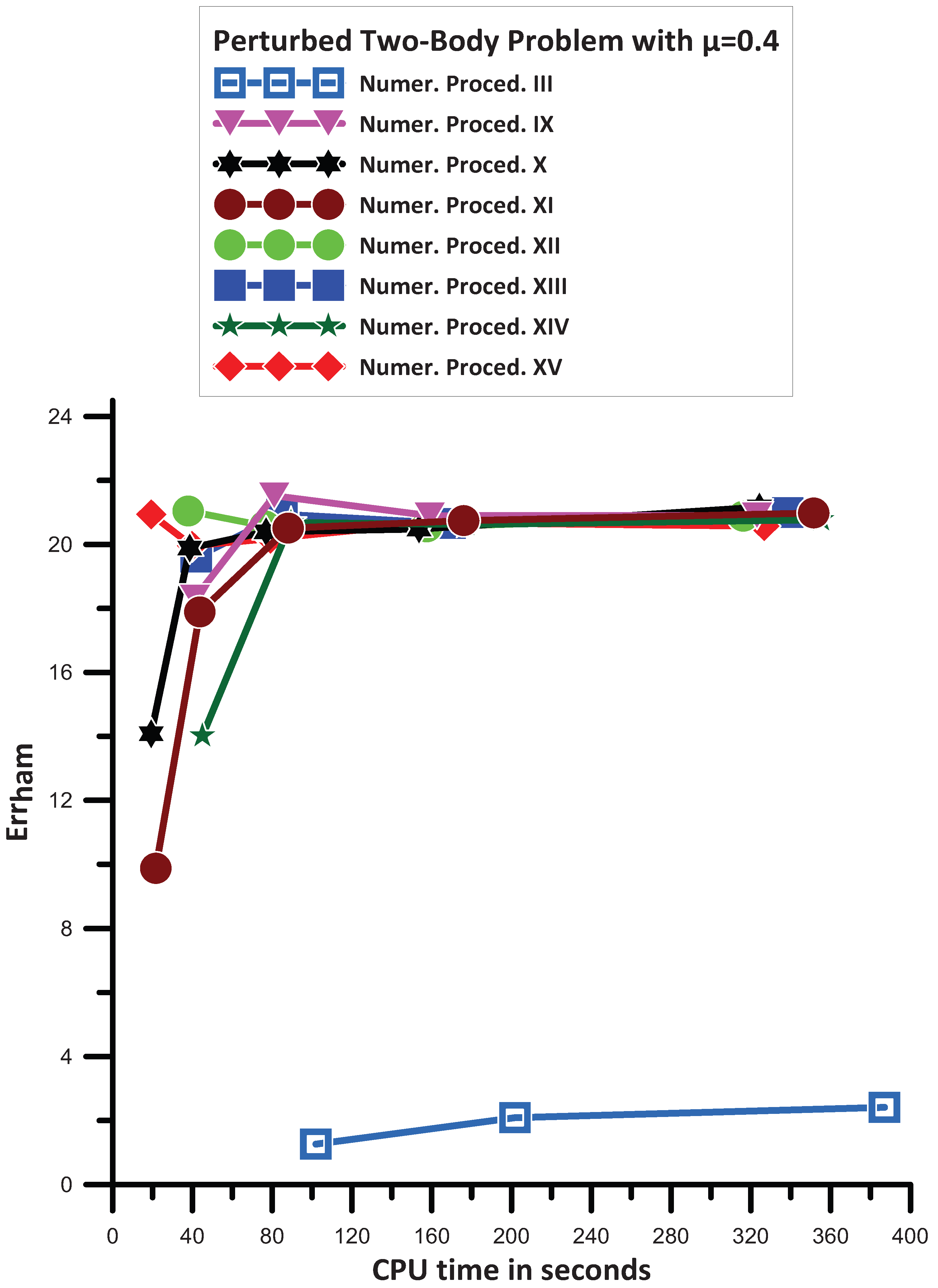
11.7. Perturbed Two–Body Gravitational Problem-Case $\mu =0.4$

The perturbed two–body Kepler’s problem is considered:

$$\begin{array}{c}\hfill {\mathrm{\Phi }}_1^{″}\left(x\right)=-{\displaystyle \frac{{\mathrm{\Phi }}_1\left(x\right)}{{\left({\mathrm{\Phi }}_1{\left(x\right)}^2+{\mathrm{\Phi }}_2{\left(x\right)}^2\right)}^{\frac{3}{2}}}}-\mu \left(\mu +2\right){\displaystyle \frac{{\mathrm{\Phi }}_1\left(x\right)}{{\left({\mathrm{\Phi }}_1{\left(x\right)}^2+{\mathrm{\Phi }}_2{\left(x\right)}^2\right)}^{\frac{5}{2}}}},\\ \hfill {\mathrm{\Phi }}_1\left(0\right)=1,{\mathrm{\Phi }}_1^{\prime }\left(0\right)=0\\ \hfill {\mathrm{\Phi }}_2^{″}\left(x\right)=-{\displaystyle \frac{{\mathrm{\Phi }}_2\left(x\right)}{{\left({\mathrm{\Phi }}_1{\left(x\right)}^2+{\mathrm{\Phi }}_2{\left(x\right)}^2\right)}^{\frac{3}{2}}}}-\mu \left(\mu +2\right){\displaystyle \frac{{\mathrm{\Phi }}_2\left(x\right)}{{\left({\mathrm{\Phi }}_1{\left(x\right)}^2+{\mathrm{\Phi }}_2{\left(x\right)}^2\right)}^{\frac{5}{2}}}},\\ \hfill {\mathrm{\Phi }}_2\left(0\right)=0,{\mathrm{\Phi }}_2^{\prime }\left(0\right)=1+\mu .\end{array}$$

(100)

The exact solution is

$$\begin{array}{c}\hfill {\mathrm{\Phi }}_1\left(x\right)=cos(x+\mu x),\\ \hfill {\mathrm{\Phi }}_2\left(x\right)=sin(x+\mu x).\end{array}$$

(101)

For this problem, we use $\omega ={\displaystyle \frac{\sqrt{1+\mu \left(\mu +2\right)}}{{\left({\mathrm{\Phi }}_1{\left(x\right)}^2+{\mathrm{\Phi }}_2{\left(x\right)}^2\right)}^{\frac{3}{4}}}}$.

Using the techniques outlined in Section 11.1, the numerical solution to the system of Equation (100) has been found for $0\le x\le 100,000$ with $\mu =0.4$

The information in Figure 14 allows us to see the following:

• Numeric. Proced. I, Numeric. Proced. II, Numeric. Proced. IV, Numeric. Proced. V, Numeric. Proced. VI, Numeric. Proced. VII, and Numeric. Proced. VIII are divergent for the data of the specific problem;
• Numeric. Proced. III is convergent, but the given results are of low accuracy;
• Numeric. Proced. IX, Numeric. Proced. X, Numeric. Proced. XI, Numeric. Proced. XII, Numeric. Proced. XIII, Numeric. Proced. XIV, and Numeric. Proced. XV give approximately the same accuracy. The accuracy given by the above methods is high, even for large step sizes.
• For large step sizes, we have the following remarks:

  -

  Numeric. Proced. XI is more efficient than Numeric. Proced. XIV;

  -

  Numeric. Proced. IX is more efficient than Numeric. Proced. XI;

  -

  Numeric. Proced. X is more efficient than Numeric. Proced. IX;

  -

  Numeric. Proced. XIII and Numeric. Proced. X give approximately the same accuracy;

  -

  Numeric. Proced. XII is more efficient than Numeric. Proced. XIII;

  -

  Numeric. Proced. XV is more efficient than Numeric. Proced. XII.

• Based on the above, Numeric. Proced. IX, Numeric. Proced. X, Numeric. Proced. XI, Numeric. Proced. XII, Numeric. Proced. XIII, Numeric. Proced. XIV, and Numeric. Proced. XV are the most efficient for small step sizes. For large step sizes, Numeric. Proced. XV is the most efficient.

Taking everything into consideration, the most effective methodologies shown here are:

• The methodology which is laid out in Section 9 that focuses on the vanishing of phase lag and amplification factor, as well as the eradication of their first derivatives.
• The methodology which is laid out in Section 6 that focuses on the vanishing of phase lag and amplification factor (the phase-fitted and amplification-fitted method).
• The methodology which is laid out in Section 7 that focuses on the vanishing of phase lag and amplification factor (the phase-fitted and amplification-fitted method) as well as the eradication of the first derivative of the phase lag.
• The methodology which is laid out in Section 8 that focuses on the vanishing of phase lag and amplification factor (the phase-fitted and amplification-fitted method) as well as the eradication of the first derivative of the amplification factor.

Finding the optimal value of the parameter v determines the efficacy of frequency-dependent algorithms, such as the recently proposed ones. Many problems have clear definitions for this decision in the problem model. There are methods in the literature for determining the parameter v that have been proposed for situations when this is not straightforward (see [39,40]).

11.8. High-Order Ordinary Differential Equations and Partial Differential Equations

When applying the recently introduced techniques to solve systems of high-order ordinary differential equations, it is important to remember that there are already established ways to simplify such systems into first-order differential equations. Some examples of such methods include substituting variables, adding new variables, rewriting the system with new variables for each derivative, and so on (refer to [41] for more information).

It should be noted that there are already established methods for reducing a system of partial differential equations to a system of first-order differential equations, such as the characteristics method (refer to [42]), which can be used to solve systems of partial differential equations using the newly introduced techniques mentioned earlier.

12. Conclusions

Our goal in this work was to examine how the numerical approaches’ efficiency is affected by the phase lag and amplification factor derivatives. In light of the above, we laid out a number of approaches to efficient method creation based on the phase lag and/or amplification factor derivatives.Particularly, we established procedures for the following:

• Methodology which includes the elimination of the derivatives of the phase lag;
• Methodology which includes the elimination of the derivatives of the amplification factor;
• Methodology which includes the elimination of the derivatives of the phase lag and the derivatives of the amplification factor.

Several multistep approaches were created using the methodologies stated above. The Adams–Bashforth fourth algebraic order method and the Adams-Bashforth fifth algebraic order method served as our foundational approaches.

In order to evaluate the efficacy of the aforementioned methodologies, they were applied to several problems involving oscillating solutions.

All our calculations adhered to the IEEE Standard 754 and were executed on a personal computer featuring an x$86--64$ compatible architecture and utilizing a quadruple precision arithmetic data type consisting of 64 bits.

References

1. Landau, L.D.; Lifshitz, F.M. Quantum Mechanics; Pergamon: New York, NY, USA, 1965. [Google Scholar]
2. Prigogine, I.; Rice, S.A. (Eds.) Advances in Chemical Physics Vol. 93: New Methods in Computational Quantum Mechanics; John Wiley & Sons: Hoboken, NJ, USA, 1997. [Google Scholar]
3. Simos, T.E. Numerical Solution of Ordinary Differential Equations with Periodical Solution. Ph.D. Dissertation, National Technical University of Athens, Athens, Greece, 1990. (In Greek). [Google Scholar]
4. Ixaru, L.G. Numerical Methods for Differential Equations and Applications; Book Series: Mathematics and Its Applications; Springer: Dordrecht, The Netherlands, 1984; ISBN 978-90-277-1597-5. [Google Scholar]
5. Quinlan, G.D.; Tremaine, S. Symmetric multistep methods for the numerical integration of planetary orbits. Astron. J. 1990, 100, 1694–1700. [Google Scholar] [CrossRef]
6. Lyche, T. Chebyshevian multistep methods for ordinary differential equations. Numer. Math. 1972, 10, 65–75. [Google Scholar] [CrossRef]
7. Konguetsof, A.; Simos, T.E. On the construction of Exponentially-Fitted Methods for the Numerical Solution of the Schrödinger Equation. J. Comput. Meth. Sci. Eng. 2001, 1, 143–165. [Google Scholar] [CrossRef]
8. Simos, T.E. Atomic Structure Computations in Chemical Modelling: Applications and Theory; Hinchliffe, A., UMIST, Eds.; The Royal Society of Chemistry: Washington, DC, USA, 2000; pp. 38–142. [Google Scholar]
9. Simos, T.E.; Vigo-Aguiar, J. On the construction of efficient methods for second order IVPs with oscillating solution. Int. J. Mod. Phys. C 2001, 10, 1453–1476. [Google Scholar] [CrossRef]
10. Dormand, J.R.; El-Mikkawy, M.E.A.; Prince, P.J. Families of Runge-Kutta-Nyström formulae. IMA J. Numer. Anal. 1987, 7, 235–250. [Google Scholar] [CrossRef]
11. Franco, J.M.; Gomez, I. Some procedures for the construction of high-order exponentially fitted Runge-Kutta-Nyström Methods of explicit type. Comput. Phys. Commun. 2013, 184, 1310–1321. [Google Scholar] [CrossRef]
12. Franco, J.M.; Gomez, I. Accuracy and linear Stability of RKN Methods for solving second-order stiff problems. Appl. Numer. Math. 2009, 59, 959–975. [Google Scholar] [CrossRef]
13. Chien, L.K.; Senu, N.; Ahmadian, A.; Ibrahim, S.N.I. Efficient Frequency-Dependent Coefficients of Explicit Improved Two-Derivative Runge-Kutta Type Methods for Solving Third- Order IVPs. Pertanika J. Sci. Technol. 2023, 31, 843–873. [Google Scholar] [CrossRef]
14. Zhai, W.J.; Fu, S.H.; Zhou, T.C.; Xiu, C. Exponentially-fitted and trigonometrically-fitted implicit RKN methods for solving y"=f(t,y). J. Appl. Math. Comput. 2022, 68, 1449–1466. [Google Scholar] [CrossRef]
15. Fang, Y.L.; Yang, Y.P.; You, X. An explicit trigonometrically fitted Runge-Kutta method for stiff and oscillatory problems with two frequencies. Int. J. Comput. Math. 2020, 97, 85–94. [Google Scholar] [CrossRef]
16. Dormand, J.R.; Prince, P.J. A family of embedded Runge-Kutta formulae. J. Comput. Appl. Math. 1980, 6, 19–26. [Google Scholar] [CrossRef]
17. Kalogiratou, Z.; Monovasilis, T.; Psihoyios, G.; Simos, T.E. Runge–Kutta type methods with special properties for the numerical integration of ordinary differential equations. Phys. Rep. 2014, 536, 75–146. [Google Scholar] [CrossRef]
18. Anastassi, Z.A.; Simos, T.E. Numerical multistep methods for the efficient solution of quantum mechanics and related problems. Phys. Rep. 2009, 482–483, 1–240. [Google Scholar] [CrossRef]
19. Chawla, M.M.; Rao, P.S. A Noumerov-Type Method with Minimal Phase-Lag for the Integration of 2nd Order Periodic Initial-Value Problems. J. Comput. Appl. Math. 1984, 11, 277–281. [Google Scholar] [CrossRef]
20. Gr, L. Ixaru and M. Rizea, A Numerov-like scheme for the numerical solution of the Schrödinger equation in the deep continuum spectrum of energies. Comput. Phys. Commun. 1980, 19, 23–27. [Google Scholar]
21. Raptis, A.D.; Allison, A.C. Exponential-fitting Methods for the numerical solution of the Schrödinger equation. Comput. Phys. Commun. 1978, 14, 1–5. [Google Scholar] [CrossRef]
22. Wang, Z.; Zhao, D.; Dai, Y.; Wu, D. An improved trigonometrically fitted P-stable Obrechkoff Method for periodic initial-value problems. Proc. R. Soc.-Math. Phys. Eng. Sci. 2005, 461, 1639–1658. [Google Scholar] [CrossRef]
23. Wang, C.; Wang, Z. A P-stable eighteenth-order six-Step Method for periodic initial value problems. Int. J. Mod. Phys. C 2007, 18, 419–431. [Google Scholar] [CrossRef]
24. Shokri, A.; Khalsaraei, M.M. A new family of explicit linear two-step singularly P-stable Obrechkoff methods for the numerical solution of second-order IVPs. Appl. Math. Comput. 2020, 376, 125116. [Google Scholar] [CrossRef]
25. Abdulganiy, R.I.; Ramos, H.; Okunuga, S.A.; Majid, Z.A. A trigonometrically fitted intra-step block Falkner method for the direct integration of second-order delay differential equations with oscillatory solutions. Afr. Mat. 2023, 34, 36. [Google Scholar] [CrossRef]
26. Lee, K.C.; Senu, N.; Ahmadian, A.; Ibrahim, S.N.I. High-order exponentially fitted and trigonometrically fitted explicit two-derivative Runge-Kutta-type methods for solving third-order oscillatory problems. Math. Sci. 2022, 16, 281–297. [Google Scholar] [CrossRef]
27. Fang, Y.L.; Huang, T.; You, X.; Zheng, J.; Wang, B. Two-frequency trigonometrically-fitted and symmetric linear multi-step methods for second-order oscillators. J. Comput. Appl. Math. 2021, 392, 113312. [Google Scholar] [CrossRef]
28. Chun, C.; Neta, B. Trigonometrically-Fitted Methods: A Review. Mathematics 2019, 7, 1197. [Google Scholar] [CrossRef]
29. Simos, T.E. A New Methodology for the Development of Efficient Multistep Methods for First–Order IVPs with Oscillating Solutions. Mathematics 2024, 12, 504. [Google Scholar] [CrossRef]
30. Simos, T.E. Efficient Multistep Algorithms for First–Order IVPs with Oscillating Solutions: II Implicit and Predictor—Corrector Algorithms. Symmetry 2024, 16, 508. [Google Scholar] [CrossRef]
31. Saadat, H.; Kiyadeh, S.H.H.; Karim, R.G.; Safaie, A. Family of phase fitted 3-step second-order BDF methods for solving periodic and orbital quantum chemistry problems. J. Math. Chem. 2024, 62, 1223–1250. [Google Scholar] [CrossRef]
32. Stiefel, E.; Bettis, D.G. Stabilization of Cowell’s method. Numer. Math. 1969, 13, 154–175. [Google Scholar] [CrossRef]
33. Fehlberg, E. Classical Fifth-, Sixth-, Seventh-, and Eighth-order Runge-Kutta Formulas with Stepsize Control. NASA Technical Report 287 (1968). Available online: https://ntrs.nasa.gov/api/citations/19680027281/downloads/19680027281.pdf (accessed on 12 December 2022).
34. Cash, J.R.; Karp, A.H. A variable order Runge–Kutta method for initial value problems with rapidly varying right-hand sides. ACM Trans. Math. Softw. 1990, 16, 201–222. [Google Scholar] [CrossRef]
35. Franco, J.M.; Palacios, M. High-order P-stable multistep methods. J. Comput. Appl. Math. 1990, 30, 1–10. [Google Scholar] [CrossRef]
36. Petzold, L.R. An efficient numerical method for highly oscillatory ordinary differential equations. SIAM J. Numer. Anal. 1981, 18, 455–479. [Google Scholar] [CrossRef]
37. Simos, T.E. New Open Modified Newton Cotes Type Formulae as Multilayer Symplectic Integrators. Appl. Math. Model. 2013, 37, 1983–1991. [Google Scholar] [CrossRef]
38. Franco, J.; Gómez, I. Trigonometrically–fitted nonuliear two–step methods for solving second order oscillatory IVPs. Appl. Math. Comput. 2014, 232, 643–657. [Google Scholar]
39. Ramos, H.; Vigo-Aguiar, J. On the frequency choice in trigonometrically fitted methods. Appl. Math. Lett. 2010, 23, 1378–1381. [Google Scholar] [CrossRef]
40. Ixaru, L.G.; Berghe, G.V.; De Meyer, H. Frequency evaluation in exponential fitting multistep algorithms for ODEs. J. Comput. Appl. Math. 2002, 140, 423–434. [Google Scholar] [CrossRef]
41. Boyce, W.E.; DiPrima, R.C.; Meade, D.B. Elementary Differential Equations and Boundary Value Problems, 11th ed.; John Wiley & Sons: Hoboken, NJ, USA, 2017; NJ07030-5774. [Google Scholar]
42. Evans, L.C. Partial Differential Equations, 2nd ed.; American Mathematical Society: Providence, RI, USA, 2010; Chapter 3; pp. 91–135. [Google Scholar]
Figure 1. Stability region for the Adams–Bashforth method developed in Section 4.
Axioms 13 00514 g001
Figure 2. Stability region for the Adams–Bashforth method developed in Section 5.
Axioms 13 00514 g002
Figure 3. Stability region for the classical fifth-order Adams–Bashforth method.
Axioms 13 00514 g003
Figure 4. Stability region for the Adams–Bashforth method developed in Section 6.
Axioms 13 00514 g004
Figure 5. Stability region for the Adams–Bashforth method developed in Section 7.
Axioms 13 00514 g005
Figure 6. Stability region for the Adams–Bashforth method developed in Section 8.
Axioms 13 00514 g006
Figure 7. Stability region for the Adams–Bashforth method developed in Section 9.
Axioms 13 00514 g007
Figure 8. Numerical results for the problem of Stiefel and Bettis [32].
Axioms 13 00514 g008
Figure 9. Numerical results for the problem of Franco and Palacios [35].
Axioms 13 00514 g009
Figure 10. Numerical results for the nonlinear problem of [36].
Axioms 13 00514 g010
Figure 11. Numerical results for the Nonlinear Orbital problem of [37].
Axioms 13 00514 g011
Figure 12. Numerical results for the semi−linear problem of Franco and Gómez [38].
Axioms 13 00514 g012
Figure 13. Numerical results for two-body gravitational problem (Kepler’s plane problem).
Axioms 13 00514 g013
Figure 14. Numerical results for perturbed two-body gravitational problem (perturbed Kepler’s problem) with μ = 0.4 .
Axioms 13 00514 g014
Disclaimer/Publisher’s Note: The statements, opinions and data contained in all publications are solely those of the individual author(s) and contributor(s) and not of MDPI and/or the editor(s). MDPI and/or the editor(s) disclaim responsibility for any injury to people or property resulting from any ideas, methods, instructions or products referred to in the content.