Abstract
In this paper, a parametric method for proving inequalities is described. The method is based on associating a considered inequality with the corresponding stratified family of functions. Many inequalities from the theory of analytic inequalities can be interpreted using families of functions that are stratified with respect to some parameter. By discussing the sign of the functions from the family by the parameter according to which the family is stratified, inequalities are obtained that contain the best possible constants, if they exist. The application of this method is demonstrated for four inequalities: the Cusa–Huygens inequality, the Wilker-type inequality and the two Mitrinović–Adamović-type inequalities. Significantly simpler proofs and improvements of all these inequalities are provided.
MSC:
26D05; 26D07
1. Introduction
In the theory of analytic inequalities, authors often give and prove improvements to some well-known inequalities. It has been shown in previous papers [1,2,3,4,5,6] that, in many cases, those inequalities can be considered through the concept of stratified families of functions [1].
In the following, we will specify the concept of the stratification of a family of functions over a real subset. We start with a family of functions defined for values of the argument for some () and parameter values for some (). The family of functions is increasingly stratified at a point if
and, conversely, the family of functions is decreasingly stratified at a point if
The family of functions is increasingly (decreasingly) stratified on a set if it is increasingly (decreasingly) stratified at every point in the set . Note that stratified families of functions appear in some mathematical problems in engineering [7,8,9,10].
The paper is divided into an introduction, three sections and a conclusion. Some new results are given within each section. In Section 2, we provide a brief overview of one method for proving mixed trigonometric polynomial inequalities over some interval [11]. This method is used in Section 4. The parametric method, based on the concept of stratification, is the subject of Section 3. Applications of the method in the theory of analytic inequalities are given in Section 4. In Section 3 and Section 4, specific choices of sets and for stratified families of functions are considered in accordance with the observed problems.
2. On a Sign of Mixed Trigonometric Polynomial Functions
In this section, we outline a method for proving mixed trigonometric polynomial (MTP) inequalities
where is an MTP function over a non-empty set given by
where , and . Note that these MTP functions are continuous on . Additionally, if is a set of the form , , , , where , then these MTP functions are differentiable any number of times on . Regarding MTP functions and inequalities, see [6,11,12,13,14,15,16,17].
In the following, we provide a brief description of the method for proving MTP inequalities according to [6,11]. As an application of this method, we will present methods for isolating zeros and extrema of MTP functions that have not been considered before.
2.1. A Positivity of MTP Functions
The MTP function (1), by applying substitutions from Table 1 [6,13] to each addend of the function , can be transformed into the equivalent form given by
where , , , or , and , for . Notice that the expression of an MTP function in terms of multiple angles (2) does not contain any powers or products of trigonometric functions.
For a real function , , a real polynomial is an upward polynomial approximation on , if it holds that
and, conversely, a real polynomial is a downward polynomial approximation on , if it holds that
A method for proving an MTP inequality
on is described in [11] for , . In that paper, the proof of the positivity of an MTP function is based on determining a downward polynomial approximation with respect to the observed MTP function such that
, where is a bounded interval.
Note that if the MTP inequality (3) is considered on the interval , an examination of the positivity of the sign of the MTP function can also be performed at the endpoints a and b. In this way, it is potentially possible to extend the inequality (3) to , or .
In [11], upper and lower bounds of the MTP functions were considered using Maclaurin approximations for the sine and cosine functions. Generally, for analytic functions, the problem of determining upper and lower bounds and approximation errors can be approached using some other methods as well (see for example [18,19,20,21,22]).
To obtain a downward polynomial approximation of the MTP function , according to [6,11], we approximate each addend of the function (2) using upward and downward Maclaurin approximations of the sine and cosine functions that are given in Lemmas 1.1 and 1.2 from [11]. Therefore, we obtain a real polynomial such that
, holds. If for a such polynomial , it holds that
, then
.
Note that in Section 4, we denote the Taylor expansion of order n of some analytic function in the neighbourhood of some point a by .
It is well known that Sturm’s theorem gives the number of zeros of a real polynomial function on a real segment, provided that the polynomial has no zeros at the endpoints of that segment ([23], Theorem 4.2 [24]). From a computational standpoint, the question arises regarding the effectiveness of the execution of Sturm’s algorithm. In [24], it has been shown that for a polynomial with rational coefficients on a segment with rational endpoints such that the polynomial does not have a zero at the endpoints of the segment, Sturm’s algorithm is executed effectively. In Section 4, the considered MTP functions and the corresponding polynomials have rational coefficients and are examined on a segment whose endpoints do not have to be rational numbers. If some endpoint is not a rational number, the proof is performed over an extended segment with rational endpoints.
2.2. Isolation Methods
In [25], a method for isolating intervals on which there are zeros of MTP functions is described and implemented. However, the computer implementation of this algorithm in Maple from [25] does not display all the steps that allow users to control and verify the proof. Therefore, in this subsection, we provide methods for isolating zeros and extrema of MTP functions based on the method for proving MTP inequalities from Section 2.1. The use of these methods allows the observation of all the steps in the proof process, i.e., verification.
2.2.1. A Method for Isolating Zeros of an MTP Function
Let us consider MTP functions on the segment , . The following assertion evidently holds:
Theorem 1
(A method for isolating zeros). If there exist points such that , satisfying the conditions:
- 1.
- f has a constant sign on and on under the condition that ;
- 2.
- has a constant sign on ;
then the MTP function has exactly one zero on the interval , more precisely, on the subinterval .
Remark 1.
The previous theorem holds for any differentiable function f over the segment . By choosing f to be an MTP function, we can verify conditions 1 and 2 using the method for proving MTP inequalities from Section 2.1.
Note that for the functions , we do not provide a selection procedure for and . If concrete values for and are determined that satisfy conditions 1 and 2 using the method for proving MTP inequalities, then we have proof of the existence of exactly one zero and the isolation of the subinterval where the zero is located.
This method cannot be applied to isolate double zeros, i.e., zeros of the even multiplicity. However, these zeros also represent local extrema of the functions. Therefore, it is possible to isolate them using the method for isolating extrema (Section 2.2.2).
If an MTP function is a non-zero function, then on a bounded interval, it has finitely many zeros. Thus, it is possible to consider a method for isolating all zeros on some bounded interval on which there is more than one zero in a similar manner.
2.2.2. A Method for Isolating Extrema of an MTP Function
Let us consider MTP functions on the segment , . The following assertion evidently holds:
Theorem 2
(A method for isolating extrema). If there exist points such that , satisfying the conditions:
- 1.
- has a constant sign on and on under the condition that ;
- 2.
- has a constant sign on ;
then the MTP function has exactly one extremum on the interval , more precisely, on the subinterval .
Remark 2.
The previous theorem holds for any two times differentiable function f over the segment . By choosing f to be an MTP function, we can verify conditions 1 and 2 using the method for proving MTP inequalities from Section 2.1.
If has a constant sign on , then, to establish the existence of exactly one extremum and isolate the subinterval where it lies, it is sufficient to prove that there exist points such that and that .
If in the condition 2, it holds that on , then the function has a minimum, whereas if holds on , the function has a maximum. For the functions , we do not provide a selection procedure for and . If concrete values for and are determined that satisfy conditions 1 and 2 using the method for proving MTP inequalities, then we have proof of the existence of exactly one extremum and the isolation of the subinterval where the extremum is located.
Note that the described method for isolating an extremum of an MTP function is identical to the method for isolating a zero of the odd multiplicity of the MTP function .
If an MTP function is not constant, then on a bounded interval, it has finitely many extrema. Thus, it is possible to consider a method for isolating all extrema on some bounded interval on which there is more than one extremum in a similar manner.
3. On the Parametric Method
In this section, the parametric method for proving inequalities will be described. Let be a family of functions that takes real values for the argument () and the parameter (). Let us observe for fixed the equation
with respect to the parameter p. In the general case, this equation may have no solution with respect to . For us, it is of particular interest to identify families for which there exists a solution with respect to , for each , especially those where the solution is unique.
With the following assertion, we provide some sufficient conditions such that for a family of functions , the equation has a solution with respect to p.
Theorem 3.
Let be a family of functions with the argument , , such that for , . If:
- (a)
- and for each , , ;
- (b)
- the functions are continuous with respect to for each ;
then for each , the equation has a solution with respect to .
Proof.
The conditions (a) and (b) ensure that for each , there will be at least one solution to the equation with respect to . If , the assumption ensures that there is a solution at point a. If , the assumption ensures that there is a solution at point b. □
A family of functions , , that satisfies the conditions of the previous theorem, we denote compressed at the point a. For such a family, the following assertion holds:
Theorem 4.
A family of functions with the argument , , that is compressed at the point a and stratified on has the property that the equation has exactly one solution with respect to , , for each .
Proof.
Theorem 3 ensures the existence of a solution to the equation for each . If there were two solutions, the family of functions would not be stratified. □
Note that the solvability of the equation with respect to the parameter p, under proper conditions for the family, is also considered with the well-known Implicit Function Theorem [26].
We further consider families of functions with the argument , , and the parameter () such that there exists a continuous function for which
In the theory of analytic inequalities, there exist numerous examples of trigonometric inequalities that can be connected to families of functions that are compressed at a point such that for them there exists a continuous function g such that (4) holds over the base interval , for example [1,2,3,5,6,27,28,29,30,31,32,33,34,35,36,37,38,39,40,41].
The function g itself, such that (4) holds, may or may not be given by some specific symbolic expression. In the applications discussed in this paper, cases where g can be determined symbolically are considered.
In the following, we examine cases of stratified families of functions when g is a monotonic function and when g is not a monotonic function. The function g determines the values of the parameter p for which the functions have zeros on the observed interval. The stratification of the family provides the order of functions in that family which is used in the following.
We first consider the case when g is a monotonic function. The following assertions hold:
Theorem 5.
Let be a family of functions for and let , satisfying the following conditions:
- 1.
- the family of functions is increasingly (decreasingly) stratified on the interval ;
- 2.
- there exists a continuous monotonically increasing function that satisfies (4);
- 3.
- there exist limits and in such that .
Then, it holds:
- (i)
- If , then
- (ii)
- If , then the equality has a unique solution and it holds thatand
- (iii)
- If , then
Proof.
The function g determines the values of the parameter p for which the functions from the family have zeros on the observed interval. Based on the properties of stratified families of functions, the corresponding inequalities from and follow. The assertion is a direct consequence of the stratification and the monotonicity of the function g. □
Theorem 6.
Let be a family of functions for and let , satisfying the following conditions:
- 1.
- the family of functions is increasingly (decreasingly) stratified on the interval ;
- 2.
- there exists a continuous monotonically decreasing function that satisfies (4);
- 3.
- there exist limits and in such that .
Then, it holds:
- (i)
- If , then
- (ii)
- If , then the equality has a unique solution and it holds thatand
- (iii)
- If , then
Proof.
It is analogous to the proof of Theorem 5. □
Remark 3.
In Theorems 5 and 6, if , the case is not possible, and if , the case is not possible.
The previous two theorems can also be considered, with minor modifications, in cases when the family of functions is defined at a or b.
Next, we consider the case when g is not a monotonic function. Let us consider a function that has exactly one local minimum on the observed interval . For such a function, the following theorem holds:
Theorem 7.
Let be a family of functions for and let , satisfying the following conditions:
- 1.
- the family of functions is increasingly (decreasingly) stratified on the interval ;
- 2.
- there exists a continuous function that satisfies (4) and that is monotonically decreasing on and monotonically increasing on for some ;
- 3.
- there exist limits and in such that for:it holds that .
Then, it holds:
- (i)
- If , then
- (ii)
- If , then the equality has exactly two solutions such that , and it holds thatand
- (iii)
- If , then the equality has a unique solution .If , thenandIf , thenand
- (iv)
- If , then
Proof.
It is analogous to the proof of Theorem 5. □
Remark 4.
In Theorem 7, if , the case is not possible, and if , the cases and are not possible.
Theorem 7 considers the case when the continuous function g that satisfies (4) has exactly one local minimum on the observed interval. Analogously, it is possible to consider the case when this function has exactly one local maximum. Moreover, it is possible to analogously consider cases when this function has more than one local extremum.
4. Applications
In this section, applications of the parametric method in the theory of analytic inequalities will be demonstrated on the examples of the Cusa–Huygens inequality from [1], the Wilker-type inequality from [39,40], and the two Mitrinović–Adamović-type inequalities from [41].
All symbolic and numerical calculations in this section were performed in computer algebra system Maple 2019.
4.1. Application 1 (Cusa–Huygens Inequality)
The Cusa–Huygens inequality is given by:
Theorem 8
([1]). Let . Then, it holds that
Many authors have studied the Cusa–Huygens inequality and generalized it [1,6,27,42,43,44,45,46,47,48,49,50,51,52,53,54,55,56,57,58,59,60,61,62]. In [1], this inequality is considered using the stratified family of functions , where
for the argument .
It has been proven that the family of functions is increasingly stratified on the interval [1]. Note that the family is defined for and for , where and . Moreover, the following assertion holds:
Lemma 1.
The families of functions and are increasingly stratified on the interval .
Proof.
It holds that on the interval for or . □
Remark 5.
Note that the family of functions , , is not stratified on the interval .
We further consider the families and for . By applying Theorem 6, as the first application of the parametric method, we provide the proof of the following statement:
Statement 1.
has a unique solution and it holds that
and
Let:
Then, it holds:
- (i)
- If , then
- (ii)
- If , then the equality
- (iii)
- If , then
Proof.
The following equivalence holds:
through which we introduce the continuous function on the interval . Let us examine the monotonicity of the function on that domain. The first derivative of the function is
For the MTP function
we prove that on the interval by applying the method for proving MTP inequalities.
The MTP function in terms of multiple angles is given by
By approximating the functions and with the Maclaurin polynomials of degrees 4 and 9, respectively, and the function with the Maclaurin polynomial of degree 5 in the addend and of degree 7 in the addend , we obtain the upward polynomial approximation
of the function on the interval . It is evident that
on the interval . Hence, on ; thus, the function is decreasing on the observed interval.
Based on Lemma 1, the family of functions is increasingly stratified on the interval .
Notice that
Note that . Hence, the family of functions satisfies all the conditions of Theorem 6. Therefore, for the considered family, everything stated in , , and for of this statement holds. Let us note that
for each . Considering that the family of functions is increasingly stratified on the interval based on Lemma 1, the assertion stated in is proven for parameter values as well. □
Note that for the families of functions and , there exist values at the endpoints and . These families are compressed at the point 0. Figure 1 illustrates these families of functions and the corresponding g function for the family of functions .
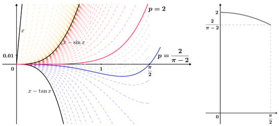
Figure 1.
Stratified families of functions from Lemma 1 with the corresponding g function; see (7).
Let us emphasize that the value was determined for the first time in [62], while the value is given by the Cusa–Huygens inequality (5). By utilizing the stratification, cases for other values of the parameter were examined and are visually depicted in Figure 1.
4.2. Application 2 (Wilker-Type Inequality)
In this paper, by the Wilker inequality, we consider the inequality from the following theorem:
Theorem 9
([63]). Let . Then, it holds that
Extensions and refinements of the Wilker inequalities have been considered in many papers [6,27,39,40,52,53,54,55,56,57,64,65,66,67,68,69,70,71,72,73,74,75,76,77,78,79,80,81,82,83,84]. In [39], the author L. Zhu proved the following statement:
Theorem 10.
Let . Then, it holds that
A new proof of Theorem 10 was given by R. Shinde, C. Chesneau, N. Darkunde, S. Ghodechor and A. Lagad in [40]. In this paper, we provide a significantly simpler proof of the previous theorem using the parametric method.
In order to provide a new proof and refine the previous theorem, we will introduce the family of functions , , where
for the argument .
The following assertion holds:
Lemma 2.
The family of functions is decreasingly stratified on the interval .
Proof.
It holds that on the interval for . □
By applying Theorem 5, we provide the proof of the following statement:
Statement 2.
has a unique solution and it holds that
and
Let:
Then, it holds:
- (i)
- If , then
- (ii)
- If , then the equality
Proof.
The following equivalence holds:
through which we introduce the continuous function on the interval . Let us examine the monotonicity of the function on that domain. The first derivative of the function is
where is the MTP function given by
Let us prove that on the interval by applying the method for proving MTP inequalities.
The MTP function in terms of multiple angles is given by
By approximating cosine functions with the Maclaurin polynomials of degree 20 in negative addends and degree 18 in positive addends, and sine functions with the Maclaurin polynomials of degree 21 in negative addends and degree 19 in positive addends, we obtain the downward polynomial approximation
of the function on the interval . By applying Sturm’s theorem to the polynomial over the extended segment with rational endpoints , it can be concluded that the polynomial has exactly one zero on that segment, which is evidently attained at the point . On the interval , the polynomial is positive since . Thus, it holds that
on the interval . Hence, on ; thus, the function is increasing on the observed interval.
Based on Lemma 2, the family of functions is decreasingly stratified on the interval .
Notice that
Note that . Hence, the family of functions satisfies all the conditions for the application of Theorem 5, which concludes the proof. □
Figure 2 illustrates the stratified family of functions from Lemma 2. Cases for some values of the real parameter p are shown, and the known constant , obtained in Theorem 10, is highlighted.
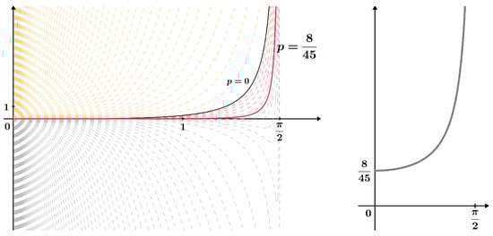
Figure 2.
Stratified family of functions from Lemma 2 with the corresponding g function; see (11).
4.3. Applications 3 and 4 (Mitrinović–Adamović-Type Inequalities)
The Mitrinović–Adamović inequality is given by:
Theorem 11
([85]). Let . Then, it holds that
Extensions and refinements of the Mitrinović–Adamović inequality have been considered in many papers [35,41,56,57,58,59,60,61,82,83,84,86,87,88,89,90,91]. In [41], the authors L. Zhu and R. Zhang gave the two following extensions:
Theorem 12.
Let . Then, it holds that
and the constants and are the best possible.
Theorem 13.
Let . Then, it holds that
and the constants and are the best possible.
Theorems 12 and 13 were proved in [41] in a manner similar to the parametric method described in this paper. However, the authors did not introduce stratified families of functions, nor did they use the method for proving MTP inequalities. In the following, we will prove Theorems 12 and 13 using the parametric method and show that this proof is simpler than the original proof from [41]. Additionally, by applying this method, we will obtain further refinements of Theorems 12 and 13 for parameter values for which these inequalities have not been previously considered.
4.3.1. Application 3
In this part, we provide new proof and refinement of Theorem 12. For this purpose, we will introduce the family of functions , , where
for the argument .
The following assertion holds:
Lemma 3.
The family of functions is decreasingly stratified on the interval .
Proof.
It holds that on the interval for . □
By applying Theorem 7, we provide the proof of the following statement:
Statement 3.
has exactly two solutions and , and it holds that
and
has a unique solution and it holds that
and
Let:
The value is the unique minimum of the function on the interval .
Then, it holds:
- (i)
- If , then
- (ii)
- If , then the equality
- (iii)
- If , then the equality
- (iv)
- If , then
Proof.
of the function on the interval . By applying Sturm’s theorem to the polynomial over the extended segment with rational endpoints , it can be concluded that the polynomial has exactly one zero on that segment, which is evidently attained at the point . On the interval , the polynomial is negative since . Thus, it holds that
on the interval .
of the function on the interval . By applying Sturm’s theorem to the polynomial over the extended segment with rational endpoints , it can be concluded that the polynomial has no zeros on that segment. On the interval , the polynomial is positive since . Thus, it holds that
on the interval .
Let us apply the method for proving MTP inequalities. The MTP function in terms of multiple angles is given by
By approximating the functions , and with the Maclaurin polynomials of degrees 16, 14 and 15, respectively, and the function with the Maclaurin polynomial of degree 15 in the addend and with the Maclaurin polynomial of degree 17 in the addend , we obtain the downward polynomial approximation
of the function on the interval . By applying Sturm’s theorem to the polynomial over the segment with rational endpoints , it can be concluded that the polynomial has no zeros on that segment. On the interval , the polynomial is positive since . Thus, it holds that
on the interval .
The following equivalence holds:
through which we introduce the continuous function on the interval . We will show that the function g has exactly one minimum on that domain. For this purpose, let us consider the first derivative of the function
where is the MTP function given by
The MTP function in terms of multiple angles is given by
Let us apply the method for isolating the zeros of the MTP function by selecting the points and on the interval such that Theorem 1 can be applied.
- 1. We prove that for and that for by applying the method for proving MTP inequalities.
- 1.1.
- By approximating the functions , , and with the Maclaurin polynomials of degrees 18, 16, 15 and 13, respectively, we obtain the downward polynomial approximation
- 1.2.
- By approximating the functions , , and with the Maclaurin polynomials of degrees 16, 14, 17 and 15, respectively, we obtain the downward polynomial approximation
- 2. We prove that for .
- It holds that
According to Theorem 1, there exists exactly one zero of the function . Given that and , the zero of the function is numerically determined as
Considering that on the interval and that on the interval , it also holds that on the interval and on the interval . Based on this, we conclude that at the point , the function g has a minimum
Based on Lemma 3, the family of functions is decreasingly stratified on the interval .
Notice that
Note that . Hence, the family of functions satisfies all the conditions for the application of Theorem 7, which concludes the proof. □
Remark 6.
It was also possible to localize the zero using the method from [25]. By using the Maple library implemented within the scope of [25], we obtain when choosing , where δ represents the maximal length of isolating intervals, without displaying all steps in the proof.
Figure 3 illustrates the stratified family of functions from Lemma 3. Cases for some values of the real parameter p are shown, and the known constants , and , obtained in Theorem 12 and Statement 3, are highlighted.
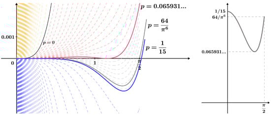
Figure 3.
Stratified family of functions from Lemma 3 with the corresponding g function; see (16).
4.3.2. Application 4
In this part, we provide new proof and refinement of Theorem 13. For this purpose, we will introduce the family of functions , , where
for the argument .
The following assertion holds:
Lemma 4.
The family of functions is decreasingly stratified on the interval .
Proof.
It holds that on the interval for . □
By applying Theorem 5, we provide the proof of the following statement:
Statement 4.
has a unique solution and it holds that
and
Let:
Then, it holds:
- (i)
- If , then
- (ii)
- If , then the equality
- (iii)
- If , then
Proof.
The following equivalence holds:
through which we introduce the continuous function on the interval . Let us examine the monotonicity of the function on that domain. The first derivative of the function is
where is the MTP function given by
Let us prove that on the interval . The MTP function in terms of multiple angles is given by
Based on the evaluation of individual addends, it is evident that
on the interval . Hence, on ; thus, the function is increasing on the observed interval.
Based on Lemma 4, the family of functions is decreasingly stratified on the interval .
Notice that
Note that . Hence, the family of functions satisfies all the conditions for the application of Theorem 5, which concludes the proof. □
Figure 4 illustrates the stratified family of functions from Lemma 4. Cases for some values of the real parameter p are shown, and the known constants and , obtained in Theorem 13, are highlighted.
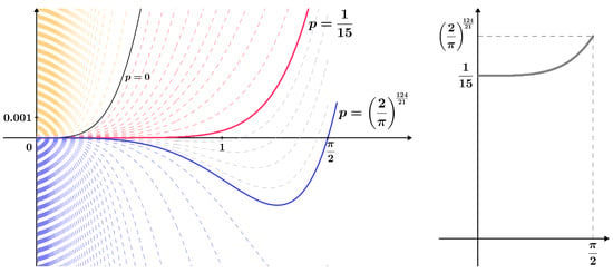
Figure 4.
Stratified family of functions from Lemma 4 with the corresponding g function; see (19).
5. Conclusions
In this paper, a method for proving inequalities via a function g, when the equivalence (4) holds and when the function g is continuous, is described. The cases when the function g is not explicitly given or when g is discontinuous will be discussed in following papers.
Let us especially emphasize that, in this paper, the concept of stratification is specified compared to [1], where it was originally introduced. With the aim of examining the monotonicity of the function g, methods for isolating zeros and extrema of MTP functions, which are based on a method for proving MTP inequalities from [11], have been described. These methods allow verification of steps as given in the proofs of the statements in this paper. The described method from [11] is also computer-implemented [92]. Therefore, it can be said that proof of inequality, in cases where examining the monotonicity of the function g is reduced to examining the positivity of MTP functions, is an algorithmically solvable problem using the parametric method as described in this paper.
Connecting inequalities with the corresponding stratified family of functions and then obtaining the corresponding g function is applicable to an exceptionally large number of inequalities in the theory of analytic inequalities [93,94,95,96,97,98,99,100]. It is particularly noteworthy to emphasize that by applying this method, additional refinements of inequalities for various parameter values can be obtained.
Author Contributions
Conceptualization, B.M. (Branko Malešević), M.M. and B.M. (Bojana Mihailović); methodology, B.M. (Branko Malešević), M.M. and B.M. (Bojana Mihailović); software, B.M. (Branko Malešević), M.M. and B.M. (Bojana Mihailović); validation, B.M. (Branko Malešević), M.M. and B.M. (Bojana Mihailović); formal analysis, B.M. (Branko Malešević), M.M. and B.M. (Bojana Mihailović); investigation, B.M. (Branko Malešević), M.M. and B.M. (Bojana Mihailović); data curation, B.M. (Branko Malešević), M.M. and B.M. (Bojana Mihailović); writing—original draft preparation, B.M. (Branko Malešević), M.M. and B.M. (Bojana Mihailović); writing—review and editing, B.M. (Branko Malešević), M.M. and B.M. (Bojana Mihailović); visualization, B.M. (Branko Malešević), M.M. and B.M. (Bojana Mihailović). All authors have read and agreed to the published version of the manuscript.
Funding
This work was financially supported by the Ministry of Science, Technological Development and Innovation of the Republic of Serbia under contract numbers: 451-03-65/2024-03/200103 (for the first and third authors) and 451-03-66/2024-03/200103 (for the second author).
Data Availability Statement
Data are contained within the article.
Acknowledgments
The authors wish to express their gratitude to the referees for their thorough reading of the paper and their valuable suggestions and comments.
Conflicts of Interest
The authors declare no conflicts of interest.
Abbreviation
The following abbreviation is used in this manuscript:
| MTP | Mixed Trigonometric Polynomial |
References
- Malešević, B.; Mihailović, B. A minimax approximant in the theory of analytic inequalities. Appl. Anal. Discret. Math. 2021, 15, 486–509. [Google Scholar] [CrossRef]
- Malešević, B.; Mihailović, B.; Nenezić Jović, M.; Mićović, M.; Milinković, L. Some generalisations and minimax approximants of D’Aurizio trigonometric inequalities. HAL 2024, hal-03550277v2. [Google Scholar]
- Malešević, B.; Jovanović, D. Frame’s Types of Inequalities and Stratification. Cubo 2024, 26, 1–19. [Google Scholar] [CrossRef]
- Malešević, B.; Mićović, M. Exponential Polynomials and Stratification in the Theory of Analytic Inequalities. J. Sci. Arts 2023, 23, 659–670. [Google Scholar] [CrossRef]
- Mićović, M.; Malešević, B. Jordan-Type Inequalities and Stratification. Axioms 2024, 13, 262. [Google Scholar] [CrossRef]
- Banjac, B.; Malešević, B.; Mićović, M.; Mihailović, B.; Savatović, M. The best possible constants approach for Wilker-Cusa-Huygens inequalities via stratification. Appl. Anal. Discret. Math. 2024, 18, 244–288. [Google Scholar] [CrossRef]
- Rahmatollahi, G.; Abreu, G. Closed-Form Hop-Count Distributions in Random Networks with Arbitrary Routing. IEEE Trans. Commun. 2012, 60, 429–444. [Google Scholar] [CrossRef]
- De Abreu, G.T.F. Jensen-Cotes Upper and Lower Bounds on the Gaussian Q-Function and Related Functions. IEEE Trans. Commun. 2009, 57, 3328–3338. [Google Scholar] [CrossRef]
- De Abreu, G.T.F. Arbitrarily Tight Upper and Lower Bounds on the Gaussian Q-Function and Related Functions. In Proceedings of the 2009 IEEE International Conference on Communications, Dresden, Germany, 14–18 June 2009. [Google Scholar]
- Ali, F.; Zahid, M.; Hou, Y.; Manafian, J.; Rana, M.A.; Hajar, A. A Theoretical Study of Reverse Roll Coating for a Non-Isothermal Third-Grade Fluid under Lubrication Approximation Theory. Math. Probl. Eng. 2022, 2022, 1–18. [Google Scholar] [CrossRef]
- Malešević, B.; Makragić, M. A Method for Proving Some Inequalities on Mixed Trigonometric Polynomial Functions. J. Math. Inequal. 2016, 10, 849–876. [Google Scholar] [CrossRef]
- Malešević, B.; Banjac, B. One method for proving polynomial inequalities with real coefficients. In Proceedings of the 28th TELFOR Conference, Belgrade, Serbia, 24–25 November 2020. [Google Scholar]
- Malešević, B.; Banjac, B. Automated Proving Mixed Trigonometric Polynomial Inequalities. In Proceedings of the 27th TELFOR Conference, Belgrade, Serbia, 26–27 November 2019. [Google Scholar]
- Yu, B.; Dong, B. A Hybrid Polynomial System Solving Method for Mixed Trigonometric Polynomial Systems. SIAM J. Numer. Anal. 2008, 46, 1503–1518. [Google Scholar] [CrossRef]
- Chen, S.; Liu, Z. Automated proving of trigonometric function inequalities using Taylor expansion. J. Syst. Sci. Math. Sci. 2016, 36, 1339–1348. (In Chinese) [Google Scholar]
- Chen, S.; Liu, Z. Automated proof of mixed trigonometric-polynomial inequalities. J. Symbolic Comput. 2020, 101, 318–329. [Google Scholar] [CrossRef]
- Chen, S.; Ge, X. Square-free factorization of mixed trigonometric-polynomials. J. Class. Anal. 2023, 22, 45–53. [Google Scholar] [CrossRef]
- Guessab, A.; Schmeisser, G. Sharp integral inequalities of the Hermite-Hadamard type. J. Approx. Theory 2002, 115, 260–288. [Google Scholar] [CrossRef]
- Dell’Accio, F.; Di Tommaso, F.; Guessab, A.; Nudo, F. A unified enrichment approach of the standard three-node triangular element. Appl. Numer. Math. 2023, 187, 1–23. [Google Scholar] [CrossRef]
- Alzer, H.; Guessab, A. An integral inequality for cosine polynomials. Appl. Math. Comput. 2014, 249, 532–534. [Google Scholar] [CrossRef]
- Chen, X.-D.; Shi, J.; Wang, Y.; Xiang, P. A New Method for Sharpening the Bounds of Several Special Functions. Results Math. 2017, 72, 695–702. [Google Scholar] [CrossRef]
- Chen, X.-D.; Wang, L.-Q.; Wang, Y.-G. A constructive method for approximating trigonometric functions and their integrals. Appl. Math. J. Chin. Univ. 2020, 35, 293–307. [Google Scholar] [CrossRef]
- Sturm, J.C.F. Mémoire sur la résolution des équations numériques. Bull. Des Sci. Ferussac 1829, 11, 419–425. [Google Scholar]
- Cutland, N. Computability: An Introduction to Recursive Function Theory; Cambridge University Press: Cambridge, UK, 1980. [Google Scholar]
- Chen, R.; Li, H.; Xia, B.; Zhao, T.; Zheng, T. Isolating all the real roots of a mixed trigonometric-polynomial. J. Symb. Comput. 2024, 121, 102250. [Google Scholar] [CrossRef]
- Rudin, W. Principles of Mathematical Analysis, 3rd ed.; McGraw-Hill: Singapore, 1976. [Google Scholar]
- Mortici, C. The natural approach of Wilker-Cusa-Huygens inequalities. Math. Inequal. Appl. 2011, 14, 535–541. [Google Scholar] [CrossRef]
- Qi, F.; Niu, D.-W.; Guo, B.-N. Refinements, Generalizations, and Applications of Jordan’s Inequality and Related Problems. J. Inequal. Appl. 2009, 2009, 271923. [Google Scholar] [CrossRef]
- Qi, F.; Guo, B.-N. On generalizations of Jordan’s inequality. Coal High. Educ. Suppl. 1993, 32–33. (In Chinese) [Google Scholar]
- Qi, F. Extensions and sharpenings of Jordan’s and Kober’s inequality. J. Math. Technol. 1996, 12, 98–102. (In Chinese) [Google Scholar]
- Deng, K. The noted Jordan’s inequality and its extensions. J. Xiangtan Min. Inst. 1995, 10, 60–63. (In Chinese) [Google Scholar]
- Jiang, W.D.; Yun, H. Sharpening of Jordan’s inequality and its applications. J. Inequalities Pure Appl. Math. 2006, 7, 1–4. [Google Scholar]
- Li, J.-L.; Li, Y.-L. On the Strengthened Jordan’s Inequality. J. Inequal. Appl. 2008, 2007, 074328. [Google Scholar] [CrossRef][Green Version]
- Huy, D.Q.; Hieu, P.T.; Van, D.T.T. New sharp bounds for sinc and hyperbolic sinc functions via cos and cosh functions. Afr. Mat. 2024, 35, 1–13. [Google Scholar] [CrossRef]
- Jiang, W.-D. New sharp inequalities of Mitrinović-Adamović type. Appl. Anal. Discret. Math. 2023, 17, 76–91. [Google Scholar] [CrossRef]
- Hung, L.-C.; Li, P.-Y. On generalization of D’Aurizio-Sándor inequalities involving a parameter. J. Math. Inequal. 2018, 12, 853–860. [Google Scholar] [CrossRef]
- Sándor, J. Extensions of D’Aurizio’s trigonometric inequality. Notes Number Theory Discret. Math. 2017, 23, 81–83. [Google Scholar]
- Li, W.-H.; Guo, B.-N. Several inequalities for bounding sums of two (hyperbolic) sine cardinal functions. Filomat 2024, 38, 3937–3943. [Google Scholar]
- Zhu, L. New inequalities of Wilker’s type for circular functions. AIMS Math. 2020, 5, 4874–4888. [Google Scholar] [CrossRef]
- Shinde, R.; Chesneau, C.; Darkunde, N.; Ghodechor, S.; Lagad, A. Revisit of an Improved Wilker Type Inequality. Pan-Am. J. Math. 2023, 2, 13. [Google Scholar] [CrossRef]
- Zhu, L.; Zhang, R. New inequalities of Mitrinović-Adamović type. Rev. R. Acad. Cienc. Exactas Fís. Nat. Ser. A Math. RACSAM 2022, 116, 1–15. [Google Scholar] [CrossRef]
- Malešević, B.; Nenezić, M.; Zhu, L.; Banjac, B.; Petrović, M. Some new estimates of precision of Cusa-Huygens and Huygens approximations. Appl. Anal. Discret. Math. 2021, 15, 243–259. [Google Scholar] [CrossRef]
- Bagul, Y.J.; Banjac, B.; Chesneau, C.; Kostić, M.; Malešević, B. New Refinements of Cusa-Huygens Inequality. Results Math. 2021, 76, 107. [Google Scholar] [CrossRef]
- Bagul, Y.J.; Chesneau, C.; Kostić, M. On the Cusa-Huygens inequality. Rev. R. Acad. Cienc. Exactas Fís. Nat. Ser. A Math. RACSAM 2021, 115, 29. [Google Scholar] [CrossRef]
- Chouikha, A.R.; Chesneau, C.; Bagul, Y.J. Some refinements of well-known inequalities involving trigonometric functions. J. Ramanujan Math. Soc. 2021, 36, 193–202. [Google Scholar]
- Bagul, Y.J.; Chesneau, C. Refined forms of Oppenheim and Cusa-Huygens type inequalities. Acta Comment. Univ. Tartu. Math. 2020, 24, 183–194. [Google Scholar] [CrossRef]
- Bagul, Y.J.; Chesneau, C.; Kostić, M. The Cusa-Huygens inequality revisited. Novi Sad J. Math. 2020, 50, 149–159. [Google Scholar]
- Dhaigude, R.M.; Chesneau, C.; Bagul, Y.J. About Trigonometric-polynomial Bounds of Sinc Function. Math. Sci. Appl. E-Notes 2020, 8, 100–104. [Google Scholar] [CrossRef]
- Zhu, L. New Inequalities of Cusa-Huygens Type. Mathematics 2021, 9, 2101. [Google Scholar] [CrossRef]
- Sándor, J.; Oláh-Gál, R. On Cusa-Huygens type trigonometric and hyperbolic inequalities. Acta Univ. Sapientiae Math. 2012, 4, 145–153. [Google Scholar]
- Wu, Y.; Bercu, G. New refinements of Becker-Stark and Cusa-Huygens inequalities via trigonometric polynomials method. Rev. R. Acad. Cienc. Exactas Fís. Nat. Ser. A Math. RACSAM 2021, 115, 87. [Google Scholar] [CrossRef]
- Chen, C.-P.; Mortici, C. The relationship between Huygens’ and Wilker’s inequalities and further remarks. Appl. Anal. Discret. Math. 2023, 17, 92–100. [Google Scholar] [CrossRef]
- Malešević, B.; Lutovac, T.; Rašajski, M.; Mortici, C. Extensions of the natural approach to refinements and generalizations of some trigonometric inequalities. Adv. Differ. Equ. 2018, 2018, 90. [Google Scholar] [CrossRef]
- Chouikha, A.R. Global approaches of trigonometric and hyperbolic inequalities. HAL 2024, hal-04637327. [Google Scholar]
- Yang, Z.-H.; Chu, Y.-M.; Song, Y.-Q.; Li, Y.-M. A Sharp Double Inequality for Trigonometric Functions and Its Applications. Abstr. Appl. Anal. 2014, 2014, 1–9. [Google Scholar] [CrossRef]
- Chen, C.-P.; Malešević, B. Sharp inequalities related to the Adamović-Mitrinović, Cusa, Wilker and Huygens results. Filomat 2023, 37, 6319–6334. [Google Scholar] [CrossRef]
- Chouikha, A.R. On natural approaches related to classical trigonometric inequalities. Open J. Math. Sci. 2023, 7, 299–320. [Google Scholar] [CrossRef]
- Chouikha, A.R. New sharp inequalities related to classical trigonometric inequalities. J. Inequal. Spec. Funct. 2020, 11, 27–35. [Google Scholar]
- Zhu, L. An unity of Mitrinovic–Adamovic and Cusa–Huygens inequalities and the analogue for hyperbolic functions. Rev. R. Acad. Cienc. Exactas Fís. Nat. Ser. A Math. RACSAM 2019, 113, 3399–3412. [Google Scholar] [CrossRef]
- Yang, Z.-H.; Chu, Y.-M. A Note on Jordan, Adamović-Mitrinović, and Cusa Inequalities. Abstr. Appl. Anal. 2014, 2014, 1–12. [Google Scholar] [CrossRef]
- Yang, Z.-H. Refinements of a two-sided inequality for trigonometric functions. J. Math. Inequal. 2013, 7, 601–615. [Google Scholar] [CrossRef]
- Malešević, B. Application of lambda method on Shafer-Fink’s inequality. Publ. Elektrotehničkog Fak.-Ser. Mat. 1997, 8, 90–92. [Google Scholar]
- Wilker, J.B. Problem E3306. Am. Math. Mon. 1989, 96, 55. [Google Scholar]
- Chen, S.; Ge, X. A solution to an open problem for Wilker-type inequalities. J. Math. Inequal. 2021, 15, 59–65. [Google Scholar] [CrossRef]
- Bercu, G. Refinements of Huygens-Wilker-Lazarović inequalities via the hyperbolic cosine polynomials. Appl. Anal. Discrete Math. 2022, 16, 91–110. [Google Scholar] [CrossRef]
- Nenezić, M.; Malešević, B.; Mortici, C. New approximations of some expressions involving trigonometric functions. Appl. Math. Comput. 2016, 283, 299–315. [Google Scholar] [CrossRef]
- Chouikha, A.R. Sharp inequalities related to Wilker results. Open J. Math. Sci. 2023, 7, 19–34. [Google Scholar] [CrossRef]
- Chouikha, A.R. On the 1-parameter trigonometric and hyperbolic inequalities chains. HAL 2024, hal-04435124. [Google Scholar]
- Zhang, B.; Chen, C.-P. Sharp Wilker and Huygens type inequalities for trigonometric and inverse trigonometric functions. J. Math. Inequal. 2020, 14, 673–684. [Google Scholar] [CrossRef]
- Chen, C.-P.; Paris, R.B. On the Wilker and Huygens-type inequalities. J. Math. Inequal. 2020, 14, 685–705. [Google Scholar] [CrossRef]
- Jiang, W.-D.; Luo, Q.-M.; Qi, F. Refinements and Sharpening of some Huygens and Wilker Type Inequalities. Turk. J. Anal. Number Theory 2014, 2, 134–139. [Google Scholar] [CrossRef][Green Version]
- Bercu, G. Refinements of Wilker-Huygens-Type Inequalities via Trigonometric Series. Symmetry 2021, 13, 1323. [Google Scholar] [CrossRef]
- Zhu, L.; Sun, Z. Refinements of Huygens- and Wilker- type inequalities. AIMS Math. 2020, 5, 2967–2978. [Google Scholar] [CrossRef]
- Guo, B.-N.; Qiao, B.-M.; Qi, F.; Li, W. On new proofs of Wilker’s inequalities involving trigonometric functions. Math. Inequal. Appl. 2003, 6, 19–22. [Google Scholar] [CrossRef]
- Zhu, L. Some New Wilker-Type Inequalities for Circular and Hyperbolic Functions. Abstr. Appl. Anal. 2009, 2009, 1–9. [Google Scholar] [CrossRef]
- Sun, Z.; Zhu, L. On New Wilker-Type Inequalities. ISRN Math. Anal. 2011, 2011, 1–7. [Google Scholar] [CrossRef][Green Version]
- Zhu, L. Wilker inequalities of exponential type for circular functions. Rev. R. Acad. Cienc. Exactas Fís. Nat. Ser. A Math. RACSAM 2021, 115, 35. [Google Scholar] [CrossRef]
- Mortici, C. A subtly analysis of Wilker inequality. Appl. Math. Comput. 2014, 231, 516–520. [Google Scholar] [CrossRef]
- Wu, S.-H.; Srivastava, H.M. A weighted and exponential generalization of Wilker’s inequality and its applications. Integral Transforms Spec. Funct. 2007, 18, 529–535. [Google Scholar] [CrossRef]
- Wu, S.-H.; Srivastava, H.M. A further refinement of Wilker’s inequality. Integral Transforms Spec. Funct. 2008, 19, 757–765. [Google Scholar] [CrossRef]
- Rašajski, M.; Lutovac, T.; Malešević, B. Sharpening and generalizations of Shafer-Fink and Wilker type inequalities: A new approach. J. Nonlinear Sci. Appl. 2018, 11, 885–893. [Google Scholar] [CrossRef][Green Version]
- Chouikha, A.R.; Chesneau, C. Contributions to trigonometric 1-parameter inequalities. HAL 2024, hal-04500965. [Google Scholar]
- Wu, S.-H.; Yue, H.-P.; Deng, Y.-P.; Chu, Y.-M. Several improvements of Mitrinović-Adamović and Lazarević’s inequalities with applications to the sharpening of Wilker-type inequalities. J. Nonlinear Sci. Appl. 2016, 9, 1755–1765. [Google Scholar] [CrossRef]
- Wu, S.-H.; Li, S.-G.; Bencze, M. Sharpened versions of Mitrinović-Adamović, Lazarević and Wilker’s inequalities for trigonometric and hyperbolic functions. J. Nonlinear Sci. Appl. 2016, 9, 2688–2696. [Google Scholar] [CrossRef]
- Mitrinović, D.S.; Adamović, D.D. Sur une inégalité élémentaire où interviennent des fonctions trigonométriques. Publ. Elektrotehničkog Fak. Ser. Mat. Fiz. 1965, 149, 23–34. [Google Scholar]
- Zhu, L.; Nenezić, M. New approximation inequalities for circular functions. J. Inequal. Appl. 2018, 2018, 313. [Google Scholar] [CrossRef] [PubMed]
- Zhu, L. New Mitrinović-Adamović type inequalities. Rev. R. Acad. Cienc. Exactas Fís. Nat. Ser. A Math. RACSAM 2020, 114, 119. [Google Scholar] [CrossRef]
- Qian, G.; Chen, X.-D. Improved bounds of Mitrinović-Adamović-type inequalities by using two-parameter functions. J. Inequal. Appl. 2023, 2023, 25. [Google Scholar] [CrossRef]
- Sándor, J. Refinements of the Mitrinović-Adamović inequality, with application. Notes Number Theory Discret. Math. 2017, 23, 4–6. [Google Scholar]
- Wu, S.; Baricz, Á. Generalizations of Mitrinović, Adamović and Lazarević’s inequalities and their applications. Publ. Math. Debr. 2009, 75, 447–458. [Google Scholar] [CrossRef]
- Zhu, L. Sharp inequalities of Mitrinovic-Adamovic type. Rev. R. Acad. Cienc. Exactas Fís. Nat. Ser. A Math. RACSAM 2019, 113, 957–968. [Google Scholar] [CrossRef]
- Banjac, B. System for Automatic Proving of Some Classes of Analytic Inequalities. Ph.D. Thesis, School of Electrical Engineering, University of Belgrade, Belgrade, Serbia, 2019. (In Serbian). [Google Scholar]
- Nenezić Jović, M. Stratified Families of Functions in the Theory of Analytical Inequalities with Applications. Ph.D. Thesis, School of Electrical Engineering, University of Belgrade, Belgrade, Serbia, 2023. (In Serbian). [Google Scholar]
- Mitrinović, D. Analytic Inequalities; Springer: Berlin, Germany, 1970. [Google Scholar]
- Anderson, G.D.; Vuorinen, M.; Zhang, X. Topics in Special Functions III. In Analytic Number Theory, Approximation Theory and Special Functions; Milovanović, G., Rassias, M., Eds.; Springer: New York, NY, USA, 2014; pp. 297–345. [Google Scholar]
- Cloud, M.J.; Drachman, B.C.; Lebedev, L.P. Inequalities with Applications to Engineering; Springer: Cham, Switzerland, 2014. [Google Scholar]
- Pachpatte, B.G. Analytic Inequalities: Recent Advances; Atlantis Press: Paris, France, 2012. [Google Scholar]
- Anastassiou, G.A. Intelligent Comparisons: Analytic Inequalities; Springer: Cham, Switzerland, 2016. [Google Scholar]
- Kazarinoff, N.D. Analytic Inequalities; Holt, Rinehart and Winston: New York, NY, USA, 1961. [Google Scholar]
- Qin, Y. Analytic Inequalities and Their Applications in PDEs; Birkhäuser: Cham, Switzerland, 2017. [Google Scholar]


Disclaimer/Publisher’s Note: The statements, opinions and data contained in all publications are solely those of the individual author(s) and contributor(s) and not of MDPI and/or the editor(s). MDPI and/or the editor(s) disclaim responsibility for any injury to people or property resulting from any ideas, methods, instructions or products referred to in the content. |
© 2024 by the authors. Licensee MDPI, Basel, Switzerland. This article is an open access article distributed under the terms and conditions of the Creative Commons Attribution (CC BY) license (https://creativecommons.org/licenses/by/4.0/).