Analysis of a Normalized Structure of a Complex Fractal–Fractional Integral Transform Using Special Functions

Abstract

By using the most generalized gamma function (parametric gamma function, or p-gamma function), we present the most generalized Rabotnov function, called the p-Rabotnov function. Consequently, new fractal–fractional differential and integral operators of a complex variable in an open unit disk are defined and investigated analytically and geometrically. We address some inequalities involving the generalized fractal–fractional integral operator in some spaces of analytic functions. A novel complex fractal–fractional integral transform (CFFIT) is presented. A normalization of the proposed CFFIT is observed in the open unit disk. Examples are illustrated for power series of analytic functions.

1. Introduction

The phrase “complex integral transform” encompasses a wide range of mathematical methods that include complex integrals. In physics and engineering, the Laplace transform is one of the greatest commonly utilized instances of a complicated integral transform. Recently, a number of studies that have made use of methods originally developed in a physical setting have concentrated on offering comprehensive accounts of social and environmental phenomena. Researchers’ ability to devise strategies has led to structures like these [1]. Such methods are used in movement theory, hyperactive complicated processes, complex fluid systems, chaotic complex systems, complex Lorenz-like patterns seen in optical physics, and the study of the nonclinical instability of the meteorological processes in the surrounding atmosphere [2]. Most of these complex transformations are structured by using the gamma function or are reduced by it. Numerous fields in science, mathematics, and industry use the gamma function, including integration, probability, and complex analysis. It has links to many mathematical ideas and functions, including the beta function and the digamma function, and is an important instrument in the exploration of special functions. As seen in [3], the p-gamma function (generalized gamma or parametric gamma function), also referred to as the modified gamma function, can be observed as follows:

$${\Gamma }_p\left(z\right)=\underset{m\to \infty }{\lim }{\displaystyle \frac{m!p^m{\left(mp\right)}^{\frac{z}{p}-1}}{{\left(z\right)}_{m,p}}},p>0$$

$${\left(z\right)}_{m,p}:={\displaystyle \frac{{\Gamma }_p(z+mp)}{{\Gamma }_p\left(z\right)}}.$$

and also satisfies the following properties

$$\Gamma \left(z\right)=\underset{p\to 1}{\lim }{\Gamma }_p\left(z\right);{\Gamma }_p\left(z\right)=p^{{\displaystyle \frac{z}{p}}-1}\Gamma \left({\displaystyle \frac{z}{p}}\right);{\Gamma }_p(z+p)=z{\Gamma }_p\left(z\right);{\Gamma }_p\left(p\right)=1.$$

We proceed to define the p-Rabotnov function by using ${\Gamma }_p$ as follows:

$$\begin{array}{cc}\hfill {\left[{\mathrm{R}}_{\kappa }\right]}_p\left(\lambda z^{\kappa /p}\right)& =\sum _{n=0}^{\infty }\left({\displaystyle \frac{{\lambda }^n{z}^{\frac{(n+1)(\kappa /p+1)}{p}-1}}{{\Gamma }_p\left[(n+1)(\kappa /p+1)\right]}}\right),\lambda ,\kappa \in \mathbb{R},p>0\hfill \\ \hfill & =\sum _{n=0}^{\infty }\left({\displaystyle \frac{{\lambda }^n{z}^{\frac{(n+1)(\kappa /p+1)}{p}-1}}{p^{\frac{(n+1)(\kappa /p+1)}{p}-1}\Gamma \left[\frac{(n+1)(\kappa /p+1)}{p}\right]}}\right)\hfill \\ \hfill & ={\left({\displaystyle \frac{z}{p}}\right)}^{(\kappa /p+1)/p-1}\sum _{n=0}^{\infty }\left({\displaystyle \frac{{\left[\lambda {(z/p)}^{\frac{\kappa /p+1}{p}}\right]}^n}{\Gamma \left[\frac{n(\kappa /p+1)+(\kappa /p+1)}{p}\right]}}\right)\hfill \\ \hfill & ={\left({\displaystyle \frac{z}{p}}\right)}^{(\kappa /p+1)/p-1}{\Xi }_{\left({\displaystyle \frac{1+\kappa /p}{p}},{\displaystyle \frac{1+\kappa /p}{p}}\right)}\left({\displaystyle \frac{\lambda z^{(1+\kappa /p)/p}}{p^{(1+\kappa /p)/p}}}\right),\hfill \end{array}$$

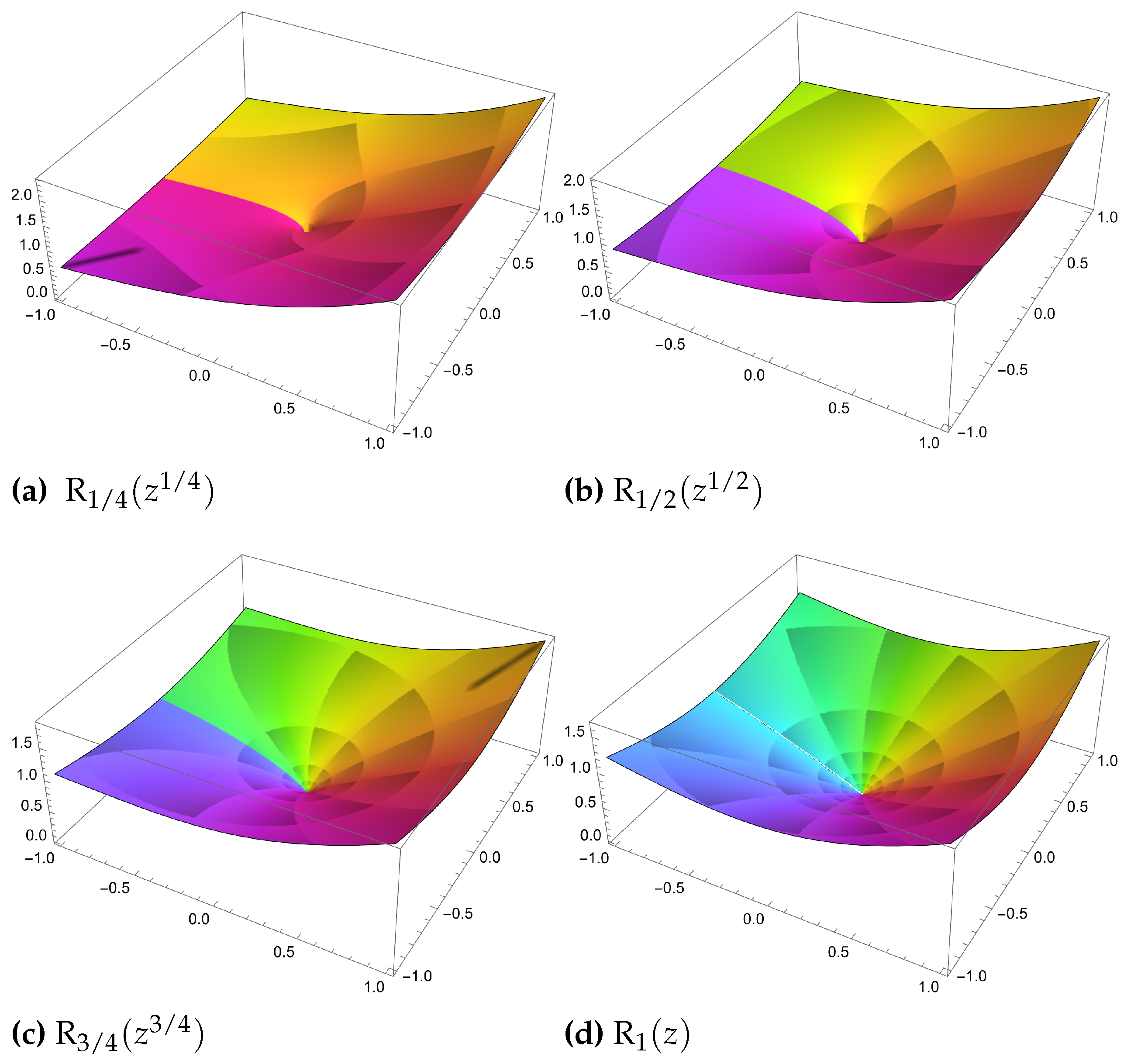
where the Mittag-Leffler function is denoted by $\Xi (.)$. Figure 1 shows a plot of the p-Rabotnov function for different values of its parameters. It is evident that we acquire the regular Rabotnov function for $p=1$ (see [4]).

Figure 1. A complex plot of the Rabotnov function for some values of $\kappa ,$ when $\lambda =1$ and $p=1$.

By using the above generalized special function, we present a set of fractal–fractional operators of a complex variable.

2. p-Fractal–Fractional Operators

The subsequent new p-fractal–fractional operators are required.

Definition 1.

The complex p-Riemann–Liouville fractal–fractional differential operator is developed for the analytic function $g\left(z\right),z\in \mathcal{I}:=\{z\in \mathbb{C}:|z|<1\}$ as follows:

$$\begin{array}{c}\hfill {}_{p\hspace{1em}}{}^{\mathcal{RL}}\Delta _z^{\kappa ,\nu }g\left(z\right)={\displaystyle \frac{d}{d{z}^{\frac{\nu }{p}}}}{\int }_0^{z}g\left(\zeta \right){\left[{\mathrm{R}}_{\kappa }\right]}_p(-\lambda {(z-\zeta )}^{{\displaystyle \frac{\kappa }{p}}})d\zeta \end{array}$$

where

$${\displaystyle \frac{dg\left(z\right)}{d{z}^{\nu /p}}}=\underset{z\to \zeta }{\lim }{\displaystyle \frac{g\left(z\right)-g\left(\zeta \right)}{z^{\nu /p}-{\zeta }^{\nu /p}}}.$$

Moreover, the Caputo formula is defined as follows:

$$\begin{array}{c}\hfill {}_p{}^{\mathcal{C}}\Delta _z^{\kappa ,\nu }g\left(z\right)={\int }_0^z{\displaystyle \frac{dg\left(\zeta \right)}{d{\zeta }^{\frac{\nu }{p}}}}{\left[{\mathrm{R}}_{\kappa }\right]}_p(-\lambda {(z-\zeta )}^{{\displaystyle \frac{\kappa }{p}}})d\zeta .\end{array}$$

Correspondingly, we define the following integral:

$${}_p\mathcal{J}_z^{\kappa ,\nu }g\left(z\right):=\nu {\int }_0^{z}g\left(\zeta \right){\left[{\mathrm{R}}_{\kappa }\right]}_p(-\lambda {(z-\zeta )}^{{\displaystyle \frac{\kappa }{p}}})d\zeta .$$

Note that when $p=1$ and $\nu =1$, the above operators are reduced [5].

Example 1.

Let $g\left(z\right)=z^q,q\in \mathbb{R}.$ Since

$$\begin{array}{c}\hfill {\left[{\mathrm{R}}_{\kappa }\right]}_p(-\lambda {(z-\zeta )}^{{\displaystyle \frac{\kappa }{p}}})={\left({\displaystyle \frac{(z-\zeta )}{p}}\right)}^{(\kappa /p+1)/p-1}{\Xi }_{\left({\displaystyle \frac{1+\kappa /p}{p}},{\displaystyle \frac{1+\kappa /p}{p}}\right)}\left({\displaystyle \frac{-\lambda {(z-\zeta )}^{(1+\kappa /p)/p}}{p^{(1+\kappa /p)/p}}}\right),\end{array}$$

where ${\left[{\Xi }_{.,.}\right]}_p$ is the p-Mittag-Leffler function, where

$$\begin{array}{c}\hfill {\left[{\Xi }_{\alpha ,\beta }\right]}_p\left(z\right)=\sum _{n=0}^{\infty }\left({\displaystyle \frac{z^n}{{\Gamma }_p(n\alpha +\beta )}}\right)=\sum _{n=0}^{\infty }\left({\displaystyle \frac{z^n}{p^{\frac{n\alpha +\beta }{p}-1}\Gamma \left(\frac{n\alpha +\beta }{p}\right)}}\right),\end{array}$$

clearly,

$${\displaystyle \frac{d\left(z^n\right)}{d{z}^{\nu /p}}}=\underset{z\to \zeta }{\lim }{\displaystyle \frac{\left(z^n\right)-\left({\zeta }^n\right)}{z^{\nu /p}-{\zeta }^{\nu /p}}}={\displaystyle \frac{p(n+1-\kappa ){\zeta }^{1-\nu /p-\kappa +n}}{\nu }}.$$

As a consequence, based on the definition of ${}_{p\hspace{1em}}{}^{\mathcal{RL}}\Delta _z^{\kappa ,\nu }$, with

$$\beta :=(\kappa /p+1)/p>0,q:=\varsigma -1>0,\rho :=\varsigma +\beta -1,$$

we obtain

$$\begin{array}{cc}\hfill & {}_{p\hspace{1em}}{}^{\mathcal{RL}}\Delta _z^{\kappa ,\nu }\left(z^q\right)\hfill \\ \hfill & ={\displaystyle \frac{d}{d{z}^{\frac{\nu }{p}}}}{\int }_0^z\left({\zeta }^q\right){\left({\displaystyle \frac{(z-\zeta )}{p}}\right)}^{(\kappa /p+1)/p-1}{\Xi }_{\left({\displaystyle \frac{1+\kappa /p}{p}},{\displaystyle \frac{1+\kappa /p}{p}}\right)}\left({\displaystyle \frac{-\lambda {(z-\zeta )}^{(1+\kappa /p)/p}}{p^{(1+\kappa /p)/p}}}\right)d\zeta \hfill \\ \hfill & ={\displaystyle \frac{1}{p^{\beta -1}}}{\displaystyle \frac{d}{d{z}^{\frac{\nu }{p}}}}{\int }_0^z\left({\zeta }^{\varsigma -1}\right){\left(z-\zeta \right)}^{\beta -1}{\Xi }_{\left(\beta ,\beta \right)}\left({\displaystyle \frac{-\lambda {(z-\zeta )}^{\beta }}{p^{\beta }}}\right)d\zeta \hfill \\ \hfill & ={\displaystyle \frac{1}{p^{\beta -1}}}{\displaystyle \frac{d}{d{z}^{\frac{\nu }{p}}}}\left(z^{\varsigma +\beta -1}{\Xi }_{\left(\beta ,\beta +\varsigma \right)}\left({\displaystyle \frac{-\lambda {\left(z\right)}^{\beta }}{p^{\beta }}}\right)\right)\hfill \\ \hfill & ={\displaystyle \frac{1}{\nu }}{\left({\displaystyle \frac{1}{p}}\right)}^{\beta -1}\left(p{z}^{\rho -{\displaystyle \frac{\nu }{p}}}\left(\rho {\Xi }_{(\beta ,\beta +\varsigma )}\left(-\lambda {\left({\displaystyle \frac{z}{p}}\right)}^{\beta }\right)-\lambda {\left({\displaystyle \frac{z}{p}}\right)}^{\beta }\left({\Xi }_{(\beta ,2\beta +\varsigma -1)}\left(-\lambda {\left({\displaystyle \frac{z}{p}}\right)}^{\beta }\right)\right.\right.\right.\hfill \\ \hfill & \left.\left.\left.-\rho {\Xi }_{(\beta ,2\beta +\varsigma )}\left(-\lambda {\left({\displaystyle \frac{z}{p}}\right)}^{\beta }\right)\right)\right)\right).\hfill \end{array}$$

Meanwhile, for $♭:=2-\nu /p-\kappa +q>0,$$\beta :=(\kappa /p+1)/p>0,$ we obtain

$$\begin{array}{cc}\hfill & {}_p{}^{\mathcal{C}}\Delta _z^{\kappa ,\nu }\left(z^q\right)\hfill \\ & ={\int }_0^z{\displaystyle \frac{d\left({\zeta }^q\right)}{d{\zeta }^{\nu /p}}}{\left({\displaystyle \frac{(z-\zeta )}{p}}\right)}^{(\kappa /p+1)/p-1}{\Xi }_{\left({\displaystyle \frac{1+\kappa /p}{p}},{\displaystyle \frac{1+\kappa /p}{p}}\right)}\left({\displaystyle \frac{-\lambda {(z-\zeta )}^{(1+\kappa /p)/p}}{p^{(1+\kappa /p)/p}}}\right)d\zeta \hfill \\ \hfill & =\left({\displaystyle \frac{p^{1-\beta }(q+1-\kappa )}{\nu }}\right){\int }_0^z{\zeta }^{♭-1}{\left(z-\zeta \right)}^{\beta -1}{\Xi }_{\left(\beta ,\beta \right)}\left({\displaystyle \frac{-\lambda {(z-\zeta )}^{\beta }}{p^{\beta }}}\right)d\zeta \hfill \\ \hfill & =\left({\displaystyle \frac{p^{1-\beta }(q+1-\kappa )}{\nu }}\right)\left({\Xi }_{\left(\beta ,\beta +♭\right)}\left({\displaystyle \frac{-\lambda {\left(z\right)}^{\beta }}{p^{\beta }}}\right)z^{♭+\beta -1}\right).\hfill \end{array}$$

With the following presumptions, if we use the fractal–fractional integral operator

$$\beta :=(\kappa /b+1)/b>0,q:=\varsigma -1>0,$$

we obtain

$$\begin{array}{cc}\hfill {}_p\mathcal{J}_z^{\kappa ,\nu }\left(z^q\right)& =\nu {\int }_0^z\left({\zeta }^q\right){\left[{\mathrm{R}}_{\kappa }\right]}_p(-\lambda {(z-\zeta )}^{{\displaystyle \frac{\kappa }{p}}}d\zeta \hfill \\ \hfill & =\nu {\left({\displaystyle \frac{1}{p}}\right)}^{(\kappa /p+1)/p-1}{\int }_0^z\left({\zeta }^q\right){\left(z-\zeta \right)}^{(\kappa /p+1)/p-1}{\Xi }_{\left({\displaystyle \frac{1+\kappa /p}{p}},{\displaystyle \frac{1+\kappa /p}{p}}\right)}\left({\displaystyle \frac{-\lambda {(z-\zeta )}^{(1+\kappa /p)/p}}{p^{(1+\kappa /p)/p}}}\right)d\zeta \hfill \\ \hfill & =\nu {\left({\displaystyle \frac{1}{p}}\right)}^{(\kappa /p+1)/p-1}{\int }_0^z\left({\zeta }^{\varsigma -1}\right){\left(z-\zeta \right)}^{\beta -1}{\Xi }_{\left(\beta ,\beta \right)}\left({\displaystyle \frac{-\lambda {(z-\zeta )}^{\beta }}{p^{\beta }}}\right)d\zeta \hfill \\ \hfill & =\nu {\left({\displaystyle \frac{1}{p}}\right)}^{(\kappa /p+1)/p-1}{\Xi }_{\left(\beta ,\beta +\varsigma \right)}\left({\displaystyle \frac{-\lambda {\left(z\right)}^{\beta }}{p^{\beta }}}\right)z^{\beta +\varsigma -1}\hfill \\ \hfill & =\nu {\left({\displaystyle \frac{1}{p}}\right)}^{(\kappa /p+1)/p-1}{\Xi }_{\left(\beta ,\beta +\varsigma \right)}\left({\displaystyle \frac{-\lambda {\left(z\right)}^{\beta }}{p^{\beta }}}\right)z^{\beta +q}.\hfill \end{array}$$

Integral Inequalities

This part deals with some inequalities involving ${}_p\mathcal{J}_z^{\kappa ,\nu }$.

Definition 2.

Let $\rho \ge 1.$ The Bergman space ${\mathbb{B}}^{\rho }$ is the set of all analytic functions g in the open unit disk $\mathcal{I}$ satisfying the norm

$$\begin{array}{c}\hfill {\parallel g\parallel }_{{\mathbb{B}}^{\rho }}^{\rho }={\displaystyle \frac{1}{\pi }}{\int }_{\mathcal{I}}{\left|g\right|}^{\rho }d\Lambda <\infty .\end{array}$$

Proposition 1.

Let $g\in {\mathbb{B}}^{\rho }$. If

$$\underset{z\in \mathcal{I}}{\max }\nu {\int }_0^z\left|{\left[{\mathrm{R}}_{\kappa }\right]}_p(-\lambda {(z-\zeta )}^{{\displaystyle \frac{\kappa }{p}}}\right|d\zeta \le C_{\nu ,\kappa ,p,\lambda },C_{\nu ,\kappa ,p,\lambda }\in (0,\infty )$$

then ${}_p\mathcal{J}_z^{\kappa ,\nu }g\left(z\right)\in {\mathbb{B}}^{\rho }.$

Proof. 

Our proof is based on Young’s inequality concerning integral operators.

$$\begin{array}{cc}\hfill {\parallel }_p{\mathcal{J}}_z^{\kappa ,\nu }{g\left(z\right)\parallel }_{{\mathbb{B}}^{\rho }}^{\rho }& ={\displaystyle \frac{1}{\pi }}{\int }_{\mathcal{I}}{\left|{}_p\mathcal{J}_z^{\kappa ,\nu }g\left(z\right)\right|}^{\rho }d\Lambda \hfill \\ \hfill & ={\displaystyle \frac{1}{\pi }}{\int }_{\mathcal{I}}{\left|\nu {\int }_0^{z}g\left(\zeta \right){\left[{\mathrm{R}}_{\kappa }\right]}_p(-\lambda {(z-\zeta )}^{{\displaystyle \frac{\kappa }{p}}})d\zeta \right|}^{\rho }d\Lambda \hfill \\ \hfill & ={\displaystyle \frac{\nu }{\pi }}{\int }_{\mathcal{I}}{\left|{\int }_0^{z}g\left(\zeta \right){\left[{\mathrm{R}}_{\kappa }\right]}_p(-\lambda {(z-\zeta )}^{{\displaystyle \frac{\kappa }{p}}})d\zeta \right|}^{\rho }d\Lambda \hfill \\ \hfill & \le \left(\underset{z\in \mathcal{I}}{\max }{\int }_0^z\left|{\left[{\mathrm{R}}_{\kappa }\right]}_p(-\lambda {(z-\zeta )}^{{\displaystyle \frac{\kappa }{p}}}\right|d\zeta \right)\left({\displaystyle \frac{1}{\pi }}{\int }_{\mathcal{I}}{\left|g\right|}^{\rho }d\Lambda \right)\hfill \\ \hfill & \le C_{\nu ,\kappa ,p,\lambda }{\parallel g\parallel }_{{\mathbb{B}}^{\rho }}^{\rho }.\hfill \end{array}$$

Hence, ${}_p\mathcal{J}_z^{\kappa ,\nu }g\left(z\right)\in {\mathbb{B}}^{\rho }.$ □

Definition 3.

The analytic function g in the open unit disk $\mathcal{I}$ is called in the space of the bounded analytic function ${\mathbb{L}}^{\infty },$ if it satisfies the norm

$$\begin{array}{c}\hfill {\parallel g\parallel }_{{\mathbb{L}}^{\infty }}=\underset{z\in \mathcal{I}}{\sup }\left|g\left(z\right)\right|<\infty .\end{array}$$

Proposition 2.

Let $g\in {\mathbb{L}}^{\infty }$. If

$$\underset{z\in \mathcal{I}}{\sup }\nu {\int }_0^z\left|{\left[{\mathrm{R}}_{\kappa }\right]}_p(-\lambda {(z-\zeta )}^{{\displaystyle \frac{\kappa }{p}}}\right|d\zeta \le K_{\nu ,\kappa ,p,\lambda },K_{\nu ,\kappa ,p,\lambda }\in (0,\infty )$$

then ${}_p\mathcal{J}_z^{\kappa ,\nu }g\left(z\right)\in {\mathbb{L}}^{\infty }.$

Proof. 

A computation yields

$$\begin{array}{cc}\hfill {\parallel }_p{\mathcal{J}}_z^{\kappa ,\nu }{g\left(z\right)\parallel }_{{\mathbb{L}}^{\infty }}& =\underset{z\in \mathcal{I}}{\sup }\left|{[}_p{\mathcal{J}}_z^{\kappa ,\nu }g\left(z\right)]\right|\hfill \\ \hfill & =\underset{z\in \mathcal{I}}{\sup }\left|\left[\nu {\int }_0^{z}g\left(\zeta \right){\left[{\mathrm{R}}_{\kappa }\right]}_p(-\lambda {(z-\zeta )}^{{\displaystyle \frac{\kappa }{p}}})d\zeta \right]\right|\hfill \\ \hfill & \le \left(\underset{z\in \mathcal{I}}{\sup }\left|g\left(z\right)\right|\right)\left(\underset{z\in \mathcal{I}}{\sup }\nu \left|\left[{\int }_0^z{\left[{\mathrm{R}}_{\kappa }\right]}_p(-\lambda {(z-\zeta )}^{{\displaystyle \frac{\kappa }{p}}})d\zeta \right]\right|\right)\hfill \\ \hfill & \le {\parallel g\parallel }_{{\mathbb{L}}^{\infty }}\left(\underset{z\in \mathcal{I}}{\sup }\nu \left[{\int }_0^z\left|{\left[{\mathrm{R}}_{\kappa }\right]}_p(-\lambda {(z-\zeta )}^{{\displaystyle \frac{\kappa }{p}}})\right]\right|d\zeta \right)\hfill \\ \hfill & \le K_{\nu ,\kappa ,p,\lambda }{\parallel g\parallel }_{{\mathbb{L}}^{\infty }}.\hfill \end{array}$$

Hence, ${}_p\mathcal{J}_z^{\kappa ,\nu }g\left(z\right)\in {\mathbb{L}}^{\infty }.$ □

Definition 4.

The analytic function g in the open unit disk $\mathcal{I}$ is called in the Bloch space of the analytic function $\mathbb{O},$ if it satisfies the norm

$$\begin{array}{c}\hfill {\parallel g\parallel }_{\mathbb{O}}=\underset{z\in \mathcal{I}}{\sup }{(1-|z|}^2\left)\right|g^{\prime }\left(z\right)|<\infty .\end{array}$$

Proposition 3.

Let $g\in {\mathbb{L}}^{\infty }$. If

$$\underset{z\in \mathcal{I}}{\sup }{\nu (1-|z|}^2)\left|{\left[{\mathrm{R}}_{\kappa }\right]}_p(-\lambda {(z-\zeta )}^{{\displaystyle \frac{\kappa }{p}}}\right|\le W_{\nu ,\kappa ,p,\lambda },W_{\nu ,\kappa ,p,\lambda }\in (0,\infty )$$

then ${}_p\mathcal{J}_z^{\kappa ,\nu }g\left(z\right)\in \mathbb{O}.$

Proof. 

A computation yields

$$\begin{array}{cc}\hfill {\parallel }_p{\mathcal{J}}_z^{\kappa ,\nu }{g\left(z\right)\parallel }_{\mathbb{O}}& =\underset{z\in \mathcal{I}}{\sup }{(1-|z|}^2)\left|{{[}_p{\mathcal{J}}_z^{\kappa ,\nu }g\left(z\right)]}^{\prime }\right|\hfill \\ \hfill & =\underset{z\in \mathcal{I}}{\sup }{(1-|z|}^2)\left|{\left[\nu {\int }_0^{z}g\left(\zeta \right){\left[{\mathrm{R}}_{\kappa }\right]}_p(-\lambda {(z-\zeta )}^{{\displaystyle \frac{\kappa }{p}}})d\zeta \right]}^{\prime }\right|\hfill \\ \hfill & \le \left(\underset{z\in \mathcal{I}}{\sup }\left|g\left(z\right)\right|\right)\left(\underset{z\in \mathcal{I}}{\sup }{\nu (1-|z|}^2)\left|\left[{\left[{\mathrm{R}}_{\kappa }\right]}_p(-\lambda {(z-\zeta )}^{{\displaystyle \frac{\kappa }{p}}})\right]\right|\right)\hfill \\ \hfill & \le W_{\nu ,\kappa ,p,\lambda }{\parallel g\parallel }_{{\mathbb{L}}^{\infty }}<\infty .\hfill \end{array}$$

Hence, ${}_p\mathcal{J}_z^{\kappa ,\nu }g\left(z\right)\in \mathbb{O}.$ □

3. Complex Fractal–Fractional Integral Transform (CFFIT)

Numerous fields of science and engineering use complex integral transformations, which are strong mathematical instruments. These examples demonstrate how complicated integral transforms may be applied to solve a wide range of issues in a variety of domains, offering insights into a range of phenomena and assisting in mathematical modeling and analysis.

From this perspective, we define the following CFFIT.

Definition 5.

An equivalent generator of order $\kappa ,\nu >0$, the p-fractal–fractional integral operator is created via the following structure:

$${}_p\top _z^{\kappa ,\nu }g\left(z\right):={\displaystyle \frac{\nu \lambda }{1+\frac{\lambda }{p{\Gamma }_p\left(\kappa \right)}}}{\int }_0^z{\zeta }^{{\displaystyle \frac{\kappa }{p}}-1}g\left(\zeta \right){(z-\zeta )}^{{\displaystyle \frac{\kappa }{p}}-1}d\zeta +{\displaystyle \frac{\nu \lambda z^{\frac{\nu }{p}-1}g\left(z\right)}{1+\frac{\lambda }{p{\Gamma }_p\left(\kappa \right)}}}.$$

$$\left(\lambda >0,p\ge 1,\kappa ,\nu >0,{\Gamma }_p\left(\kappa \right)=p^{{\displaystyle \frac{\kappa }{p}}-1}\Gamma ({\displaystyle \frac{\kappa }{p}}),\mathrm{Re}({(z-\zeta )}^{{\displaystyle \frac{\kappa }{p}}-1})>0\right)$$

Proposition 4.

Assume that $\mathtt{H}$ is a complex Hilbert space of analytic functions. If $g\in L^2(\mathcal{I},\mathtt{H})$ with $\mathrm{Re}\left(g\right(z\left)\right)>0$ then ${}_p\top _z^{\kappa ,\nu }g\left(z\right)$ is is accretive operator, i.e.,

$$\mathrm{Re}{\left({}_p\top _z^{\kappa ,\nu }g\left(z\right),g\left(z\right)\right)}_{L^2(\mathcal{I},\mathtt{H})}>0,\mathrm{Re}\left(z\right)>0.$$

Proof. 

Based on the assumptions of this proposition, we obtain

$$\begin{array}{cc}\hfill & \mathtt{Re}{\left({}_p\top _z^{\kappa ,\nu }g\left(z\right),g\left(z\right)\right)}_{L^2(\mathcal{I},\mathtt{H})}\hfill \\ & =\mathtt{Re}{\left({\displaystyle \frac{\nu \lambda }{1+\frac{\lambda }{p{\Gamma }_p\left(\kappa \right)}}}{\int }_0^z{\zeta }^{{\displaystyle \frac{\kappa }{p}}-1}g\left(\zeta \right){(z-\zeta )}^{{\displaystyle \frac{\kappa }{p}}-1}d\zeta +{\displaystyle \frac{\nu \lambda z^{\frac{\nu }{p}-1}g\left(z\right)}{1+\frac{\lambda }{p{\Gamma }_p\left(\kappa \right)}}},g\left(z\right)\right)}_{L^2(\mathcal{I},\mathtt{H})}\hfill \\ \hfill & ={\left({\displaystyle \frac{\nu \lambda }{1+\frac{\lambda }{p{\Gamma }_p\left(\kappa \right)}}}\mathtt{Re}\left({\int }_0^z{\zeta }^{{\displaystyle \frac{\kappa }{p}}-1}g\left(\zeta \right){(z-\zeta )}^{{\displaystyle \frac{\kappa }{p}}-1}d\zeta +{\displaystyle \frac{\nu \lambda z^{\frac{\nu }{p}-1}g\left(z\right)}{1+\frac{\lambda }{p{\Gamma }_p\left(\kappa \right)}}}\right),\mathtt{Re}\left(g\left(z\right)\right)\right)}_{L^2(\mathcal{I},\mathtt{H})}\hfill \\ \hfill & >0.\hfill \end{array}$$

where ${}_p\top _z^{\kappa ,\nu }g\left(z\right)$ is an accretive operator. □

Normalization Form

The p-fractal–fractional integral transform yields the following observation:

$$\begin{array}{cc}\hfill {}_p\top _z^{\kappa ,\nu }\left(z^q\right)& ={\displaystyle \frac{\nu \lambda }{1+\frac{\lambda }{p^{\frac{\kappa }{p}-1}\Gamma \left(\frac{\kappa }{p}\right)}}}\left({\int }_0^z{\zeta }^{{\displaystyle \frac{\kappa }{p}}-1+q}{(z-\zeta )}^{{\displaystyle \frac{\kappa }{p}}-1}d\zeta +z^{{\displaystyle \frac{\nu }{p}}-1+q}\right)\hfill \\ \hfill & ={\displaystyle \frac{\nu \lambda }{1+\frac{\lambda }{p^{\frac{\kappa }{p}-1}\Gamma \left(\frac{\kappa }{p}\right)}}}\left({\displaystyle \frac{\Gamma \left(\frac{\kappa }{p}\right)\Gamma \left(\frac{\kappa }{p}+q\right)z^{\frac{2\kappa }{p}+q-1}}{\Gamma \left(\frac{2\kappa }{p}+q\right)}}+z^{{\displaystyle \frac{\nu }{p}}-1+q}\right).\hfill \end{array}$$

Let

$$\Lambda :={\displaystyle \frac{\nu \lambda }{1+\frac{\lambda }{p^{\frac{\kappa }{p}-1}\Gamma \left(\frac{\kappa }{p}\right)}}},{\omega }_n:={\displaystyle \frac{\Gamma \left(\frac{\kappa }{p}\right)\Gamma \left(\frac{\kappa }{p}+n\right)}{\Gamma \left(\frac{2\kappa }{p}+n\right)}}.$$

Then, by setting ${}_p\top _z^{\kappa ,\nu },$ where $z\in \mathcal{I}$ in the analytic function $g\left(z\right)={\sum }_{n=0}^{\infty }{a}_n{z}^n$, we calculate the CFFIT as follows:

$$\begin{array}{cc}\hfill & {}_p\top _z^{\kappa ,\nu }g\left(z\right)=z^{2\kappa /p-1}\Lambda \sum _{n=0}^{\infty }{a}_n(1+{\omega }_n)z^n,a_0=0,\hfill \end{array}$$

where $\nu =2\kappa .$ If $g\left(z\right)$ is normalized by $g\left(0\right)=0,g^{\prime }\left(0\right)=1,$${}_p\top _z^{\kappa ,\nu }g\left(z\right)$ can be normalized as follows:

$$\begin{array}{cc}\hfill {}_p\mathbb{T}_z^{\kappa ,2\kappa }g\left(z\right)& :={\displaystyle \frac{{}_p\top _z^{\kappa ,2\kappa }\left(z+{\sum }_{n=2}^{\infty }{a}_n{z}^n\right)}{\Lambda z^{2\kappa /p-1}({\omega }_1+1)}}\hfill \\ \hfill & =z+\sum _{n=2}^{\infty }{a}_n\left({\displaystyle \frac{{\omega }_n+1}{{\omega }_1+1}}\right)z^n,\left|z\right|<1.\hfill \end{array}$$

Here, we denote the class of normalized analytic functions in $\mathcal{I}$ using $\mathcal{N}.$

Proposition 5.

Consider the operator ${}_p\mathbb{T}_z^{\kappa ,2\kappa }g\left(z\right),$ where $g\left(z\right)=z+{\sum }_{n=2}^{\infty }{a}_n{z}^n,\left|z\right|<1/2.$ If $|a_n|<{\displaystyle \frac{{\omega }_1+1}{{\omega }_n+1}}$, then ${}_p\mathbb{T}_z^{\kappa ,2\kappa }g\left(z\right)$ is convex. In addition, if $|a_n|<{\displaystyle \frac{2}{\sqrt{5}}}\left({\displaystyle \frac{{\omega }_1+1}{{\omega }_n+1}}\right)$, then ${}_p\mathbb{T}_z^{\kappa ,2\kappa }g\left(z\right)$ is starlike.

Proof. 

It is well known that [6,7]

$$\begin{array}{cc}\hfill & \left|g^{\prime }\left(z\right)-1\right|<1\Rightarrow gisconvexin\left|z\right|<{\displaystyle \frac{1}{2}}\hfill \end{array}$$

$$\begin{array}{cc}\hfill & \left|g^{\prime }\left(z\right)-1\right|<{\displaystyle \frac{2}{\sqrt{5}}}\Rightarrow gisstarlikein\left|z\right|<{\displaystyle \frac{1}{2}}.\hfill \end{array}$$

A computation implies that

$$\begin{array}{cc}\hfill \left|{\left({}_p\mathbb{T}_z^{\kappa ,2\kappa }g\left(z\right)\right)}^{\prime }-1\right|& \le \sum _{n=2}^{\infty }|a_n|\left({\displaystyle \frac{{\omega }_n+1}{{\omega }_1+1}}\right){\left|z\right|}^{n-1}\hfill \\ \hfill & \le \sum _{n=2}^{\infty }\left|a_n\right|\left({\displaystyle \frac{{\omega }_n+1}{{\omega }_1+1}}\right){\left({\displaystyle \frac{1}{2}}\right)}^{n-1}\hfill \\ \hfill & <\sum _{n=2}^{\infty }{\displaystyle \frac{1}{2^{n-1}}}=1.\hfill \end{array}$$

Thus, ${}_p\mathbb{T}_z^{\kappa ,2\kappa }g\left(z\right)$ is convex. The same is true for the second part. □

The next proposition shows the upper bound of the CFFIT in the open unit disk, when g achieves some special geometric properties. We prove that the suggested normalized operator is bounded in the open unit disk by the special generalized $\Psi -$Fox–Wright function for some geometric functions $g\left(z\right)$.

Proposition 6.

Consider the operator ${}_p\mathbb{T}_z^{\kappa ,2\kappa }g\left(z\right),$ where

$$g\left(z\right)=z+\sum _{n=2}^{\infty }{a}_n{z}^n,\left|z\right|<1.$$

If g is convex, then

$$\begin{array}{c}\hfill \left|{}_p\mathbb{T}_z^{\kappa ,2\kappa }g\left(z\right)\right|\le \left({\displaystyle \frac{r}{{\omega }_1+1}}\right)\left({}_3\Psi _1\left[\begin{array}{ccc}({\displaystyle \frac{\kappa }{p}},0)& ({\displaystyle \frac{\kappa }{p}}+1,1)& (1,1)\\ ({\displaystyle \frac{2\kappa }{p}}+1,1)\end{array};r\right]+{}_1\Psi _1\left[\begin{array}{c}(1,1)\\ (1,0)\end{array};r\right]\right).\end{array}$$

Proof. 

Since g is convex, $|a_n|<1$ for all n (see [8]). Based on the definition of ${}_p\mathbb{T}_z^{\kappa ,2\kappa }g\left(z\right),$ we obtain

$$\begin{array}{cc}\hfill \left|{}_p\mathbb{T}_z^{\kappa ,2\kappa }g\left(z\right)\right|& =\left|\sum _{n=1}^{\infty }{a}_n\left({\displaystyle \frac{{\omega }_n+1}{{\omega }_1+1}}\right)z^n\right|\hfill \\ \hfill & =\left({\displaystyle \frac{1}{{\omega }_1+1}}\right)\left|\sum _{n=1}^{\infty }{a}_n\left({\displaystyle \frac{\Gamma \left(\frac{\kappa }{p}\right)\Gamma \left(\frac{\kappa }{p}+n\right)+\Gamma \left(\frac{2\kappa }{p}+n\right)}{\Gamma \left(\frac{2\kappa }{p}+n\right)}}\right)z^n\right|\hfill \\ \hfill & \le \left({\displaystyle \frac{1}{{\omega }_1+1}}\right)\sum _{n=1}^{\infty }\left({\displaystyle \frac{\Gamma \left(\frac{\kappa }{p}\right)\Gamma \left(\frac{\kappa }{p}+n\right)+\Gamma \left(\frac{2\kappa }{p}+n\right)}{\Gamma \left(\frac{2\kappa }{p}+n\right)}}\right)\left|z^n\right|\hfill \\ \hfill & \le \left({\displaystyle \frac{1}{{\omega }_1+1}}\right)\left(\sum _{n=1}^{\infty }\left({\displaystyle \frac{\Gamma \left(\frac{\kappa }{p}\right)\Gamma \left(\frac{\kappa }{p}+n\right)\Gamma (n+1)}{\Gamma \left(\frac{2\kappa }{p}+n\right)}}\right){\displaystyle \frac{r^n}{n!}}+\sum _{n=1}^{\infty }\Gamma \left(n+1\right){\displaystyle \frac{r^n}{n!}}\right)\hfill \\ \hfill & =\left({\displaystyle \frac{r}{{\omega }_1+1}}\right)\left(\sum _{n=0}^{\infty }{\displaystyle \frac{\Gamma \left(\frac{\kappa }{p}\right)\Gamma \left(\frac{\kappa }{p}+n+1\right){\displaystyle \frac{\Gamma (n+2)}{n+1}}}{\Gamma \left(\frac{2\kappa }{p}+n+1\right)}}{\displaystyle \frac{r^n}{n!}}+\sum _{n=0}^{\infty }{\displaystyle \frac{\Gamma \left(n+2\right)}{n+1}}{\displaystyle \frac{r^n}{n!}}\right)\hfill \\ \hfill & =\left({\displaystyle \frac{r}{{\omega }_1+1}}\right)\left(\sum _{n=0}^{\infty }{\displaystyle \frac{\Gamma \left(\frac{\kappa }{p}\right)\Gamma \left(\frac{\kappa }{p}+n+1\right)\Gamma (n+1)}{\Gamma \left(\frac{2\kappa }{p}+n+1\right)}}{\displaystyle \frac{r^n}{n!}}+\sum _{n=0}^{\infty }\Gamma (n+1){\displaystyle \frac{r^n}{n!}}\right)\hfill \\ \hfill & =\left({\displaystyle \frac{r}{{\omega }_1+1}}\right)\left({}_3\Psi _1\left[\begin{array}{ccc}({\displaystyle \frac{\kappa }{p}},0)& ({\displaystyle \frac{\kappa }{p}}+1,1)& (1,1)\\ ({\displaystyle \frac{2\kappa }{p}}+1,1)\end{array};r\right]+{}_1\Psi _1\left[\begin{array}{c}(1,1)\\ (1,0)\end{array};r\right]\right)\hfill \end{array}$$

□

Proposition 7.

Consider the operator ${}_p\mathbb{T}_z^{\kappa ,2\kappa }g\left(z\right),$ where

$$g\left(z\right)=z+\sum _{n=2}^{\infty }{a}_n{z}^n,\left|z\right|<1.$$

If g is starlike, then

$$\begin{array}{c}\hfill \left|{}_p\mathbb{T}_z^{\kappa ,2\kappa }g\left(z\right)\right|\le \left({\displaystyle \frac{r}{{\omega }_1+1}}\right)\left({}_3\Psi _1\left[\begin{array}{ccc}({\displaystyle \frac{\kappa }{p}},0)& ({\displaystyle \frac{\kappa }{p}}+1,1)& (2,1)\\ ({\displaystyle \frac{2\kappa }{p}}+1,1)\end{array};r\right]+{}_1\Psi _1\left[\begin{array}{c}(2,1)\\ (1,0)\end{array};r\right]\right).\end{array}$$

Proof. 

Since g is starlike, $|a_n|<n$ for all n (see [8]). Based on the definition of ${}_p\mathbb{T}_z^{\kappa ,2\kappa }g\left(z\right),$ we obtain

$$\begin{array}{cc}\hfill \left|{}_p\mathbb{T}_z^{\kappa ,2\kappa }g\left(z\right)\right|& \le \left({\displaystyle \frac{1}{{\omega }_1+1}}\right)\sum _{n=1}^{\infty }n\left({\displaystyle \frac{\Gamma \left(\frac{\kappa }{p}\right)\Gamma \left(\frac{\kappa }{p}+n\right)+\Gamma \left(\frac{2\kappa }{p}+n\right)}{\Gamma \left(\frac{2\kappa }{p}+n\right)}}\right)\left|z^n\right|\hfill \\ \hfill & \le \left({\displaystyle \frac{1}{{\omega }_1+1}}\right)\left(\sum _{n=1}^{\infty }n\left({\displaystyle \frac{\Gamma \left(\frac{\kappa }{p}\right)\Gamma \left(\frac{\kappa }{p}+n\right)\Gamma (n+1)}{\Gamma \left(\frac{2\kappa }{p}+n\right)}}\right){\displaystyle \frac{r^n}{n!}}+\sum _{n=1}^{\infty }n\Gamma \left(n+1\right){\displaystyle \frac{r^n}{n!}}\right)\hfill \\ \hfill & =\left({\displaystyle \frac{r}{{\omega }_1+1}}\right)\left(\sum _{n=0}^{\infty }{\displaystyle \frac{\Gamma \left(\frac{\kappa }{p}\right)\Gamma \left(\frac{\kappa }{p}+n+1\right)\Gamma (n+2)}{\Gamma \left(\frac{2\kappa }{p}+n+1\right)}}{\displaystyle \frac{r^n}{n!}}+\sum _{n=0}^{\infty }\Gamma \left(n+2\right){\displaystyle \frac{r^n}{n!}}\right)\hfill \\ \hfill & =\left({\displaystyle \frac{r}{{\omega }_1+1}}\right)\left({}_3\Psi _1\left[\begin{array}{ccc}({\displaystyle \frac{\kappa }{p}},0)& ({\displaystyle \frac{\kappa }{p}}+1,1)& (2,1)\\ ({\displaystyle \frac{2\kappa }{p}}+1,1)\end{array};r\right]+{}_1\Psi _1\left[\begin{array}{c}(2,1)\\ (1,0)\end{array};r\right]\right).\hfill \end{array}$$

□

4. Special Formulas Involving CFFIT

In this section, we deal with a list of special formulas that contain the suggested CFFIT. These formulas belong to a class of analytic functions in the open unit disk (see [8]). For $ϵ>0,$ the class of analytic functions $\psi \left(z\right)$ satisfies the main conditions $\psi \left(0\right)=1$ and $\Re \left(\psi \right)>ϵ$. This class is denoted by $\Psi \left(ϵ\right).$ This class achieves the inclusion property $\Psi \left({ϵ}_m\right)\subset \cdots \subset \Psi \left({ϵ}_1\right)\subset \Psi \left(0\right)\equiv \Psi ,$ whenever $0<{ϵ}_1,\cdots <{ϵ}_m.$ Obviously, the subclasses of starlike and convex functions are in $\Psi \left(0\right).$ Moreover, two analytic functions, $\varphi$ and $\phi \in \mathcal{I}$, are subordinated, denoted by $\varphi \prec \phi$, if $\varphi \left(\mathcal{I}\right)\subset \phi \left(\mathcal{I}\right)$ and $\phi \left(0\right)=\varphi \left(0\right).$

To prove our results, we need the following preliminary [9]

Lemma 1.

For $c\in \mathbb{C}$ and positive integer n, let $\mathbb{A}[c,n]=\{h:h\left(z\right)=c+c_n{z}^n+c_{n+1}{z}^{n+1}+...\}.$

i. 

For $\wp \in \mathbb{R},$ the following relation is satisfied $\Re \left(h\left(z\right)+\wp z{h}^{\prime }\left(z\right)\right)>0⟹\Re \left(h\left(z\right)\right)>0.$ In addition, for $\wp >0$ and $h\in \mathbb{A}[1,n]$, there are two constants, ${\ell }_1>0$ and ${\ell }_2>0$, with ${\ell }_2={\ell }_2(\wp ,{\ell }_1,n)$ satisfying the relation

$$h\left(z\right)+\wp z{h}^{\prime }\left(z\right)\prec {\left[{\displaystyle \frac{1+z}{1-z}}\right]}^{{\ell }_2}\Rightarrow h\left(z\right)\prec {\left[{\displaystyle \frac{1+z}{1-z}}\right]}^{{\ell }_1}.$$

ii. 

For $\wp \in [0,1)$ and $h\in \mathbb{A}[1,n]$, there is a constant $\ell >0$ with $\ell =\ell (\wp ,n)$ such that

$$\Re \left(h^2\left(z\right)+2h\left(z\right).z{h}^{\prime }\left(z\right)\right)>\wp \Rightarrow \Re \left(h\left(z\right)\right)>\ell .$$

iii. 

If $h\in \mathbb{A}[c,n]$ with $\Re c>0$, then $\Re \left(h\left(z\right)+z{h}^{\prime }\left(z\right)+z^2{h}^{″}\left(z\right)\right)>0$; then, $\Re \left(h\right(z\left)\right)>0.$ Moreover, if $\hslash :\mathcal{I}\to \mathbb{R}$ and $\Re \left(h\left(z\right)+\hslash \left(z\right){\displaystyle \frac{z{h}^{\prime }\left(z\right)}{h\left(z\right)}}\right)>0$, then $\Re \left(h\right(z\left)\right)>0.$

Lemma 2.

Let h be a convex function with $h\left(0\right)=c,$ and let $\chi \in \mathbb{C}\setminus \left\{0\right\}$ be a complex number with $\Re \left(\chi \right)\ge 0.$ If $v\in \mathbb{A}[c,n],$ and $v\left(z\right)+{\displaystyle \frac{z}{\chi }}{v}^{\prime }\left(z\right)\prec h\left(z\right),z\in \mathcal{I},$ then $v\left(z\right)\prec L\left(z\right)\prec h\left(z\right),$ where

$$L\left(z\right)={\displaystyle \frac{1+\chi }{n{z}^{\chi /n}}}{\int }_0^{z}h\left(\tau \right){\tau }^{{\displaystyle \frac{\chi }{n}}-1}d\tau ,z\in \mathcal{I}.$$

Theorem 1.

For $g\in \mathcal{N}$, if one of the following relations is satisfied

• $\Re {\left({}_p\mathbb{T}_z^{\kappa ,2\kappa }g\left(z\right)\right)}^{\prime }>0$;
• ${{(}_p{\mathbb{T}}_z^{\kappa ,2\kappa }g\left(z\right))}^{\prime }\prec {\left({\displaystyle \frac{1+z}{1-z}}\right)}^{{\ell }_1},{\ell }_1>0,z\in \mathcal{I};$
• $\Re \left({{[}_p{\mathbb{T}}_z^{\kappa ,2\kappa }g\left(z\right)]}^{\prime }{\displaystyle \frac{{}_p\mathbb{T}_z^{\kappa ,2\kappa }g\left(z\right)}{z}}\right)>{\displaystyle \frac{\wp }{2}},\wp \in [0,1),z\in \mathcal{I};$
• $\Re \left({\displaystyle \frac{z{{[}_p{\mathbb{T}}_z^{\kappa ,2\kappa }g\left(z\right)]}^{″}}{2}}-{\displaystyle \frac{{{[}_p{\mathbb{T}}_z^{\kappa ,2\kappa }g\left(z\right)]}^{\prime }}{2}}+{\displaystyle \frac{{}_p\mathbb{T}_z^{\kappa ,2\kappa }g\left(z\right)}{z}}\right)>0,$
• $\Re \left({\displaystyle \frac{z{{[}_p{\mathbb{T}}_z^{\kappa ,2\kappa }g\left(z\right)]}^{\prime }}{2{[}_p{\mathbb{T}}_z^{\kappa ,2\kappa }g\left(z\right)]}}+{\displaystyle \frac{{[}_p{\mathbb{T}}_z^{\kappa ,2\kappa }g\left(z\right)]}{z}}\right)>{\displaystyle \frac{1}{2}}$

then ${\displaystyle \frac{{[}_p{\mathbb{T}}_z^{\kappa ,2\kappa }g\left(z\right)]}{z}}\in \Psi \left(ϵ\right)$ for the indicated $ϵ\in [0,1)$.

Proof. 

Define the following analytic function

$$v\left(z\right)={\displaystyle \frac{{[}_p{\mathbb{T}}_z^{\kappa ,2\kappa }g\left(z\right)]}{z}}\Rightarrow z{v}^{\prime }\left(z\right)+v\left(z\right)={{[}_p{\mathbb{T}}_z^{\kappa ,2\kappa }g\left(z\right)]}^{\prime }.$$

(1)

The first condition implies that $\Re (z{v}^{\prime }\left(z\right)+v\left(z\right))>0.$ Thus, according to Lemma 1.i, where $\wp =1,$ we obtain $\Re ({\displaystyle \frac{{[}_p{\mathbb{T}}_z^{\kappa ,2\kappa }g\left(z\right)]}{z}})>0$, which concludes that ${\displaystyle \frac{{[}_p{\mathbb{T}}_z^{\kappa ,2\kappa }g\left(z\right)]}{z}}\in \Psi \left(0\right)$.

The next subordination states that

$${{[}_p{\mathbb{T}}_z^{\kappa ,2\kappa }g\left(z\right)]}^{\prime }=z{v}^{\prime }\left(z\right)+v\left(z\right)\prec {\left[{\displaystyle \frac{1+z}{1-z}}\right]}^{{\ell }_1}.$$

Again according to Lemma 1.i, there is a constant $\wp >0$ with ${\ell }_2={\ell }_2(\wp )$ with

$${\displaystyle \frac{{[}_p{\mathbb{T}}_z^{\kappa ,2\kappa }g\left(z\right)]}{z}}\prec {\left({\displaystyle \frac{1+z}{1-z}}\right)}^{{\ell }_2}.$$

This implies that ${\displaystyle \frac{{[}_p{\mathbb{T}}_z^{\kappa ,2\kappa }g\left(z\right)]}{z}}\in \Psi \left(ϵ\right),ϵ\in (0,1).$

We proceed with the third relation, which yields

$$\Re \left(v^2\left(z\right)+2v\left(z\right).z{v}^{\prime }\left(z\right)\right)=2\Re \left({{[}_p{\mathbb{T}}_z^{\kappa ,2\kappa }g\left(z\right)]}^{\prime }{\displaystyle \frac{{[}_p{\mathbb{T}}_z^{\kappa ,2\kappa }g\left(z\right)]}{z}}\right)>\wp .$$

(2)

According to Lemma 1.ii, there is a constant $\ell >0$ satisfying $\Re \left(v\right(z\left)\right)>\ell$ such that $v\left(z\right)={\displaystyle \frac{{[}_p{\mathbb{T}}_z^{\kappa ,2\kappa }g\left(z\right)]}{z}}\in \Psi \left(ϵ\right)$ for some $ϵ\in (0,1).$ It follows from (2) that $\Re \left({{[}_p{\mathbb{T}}_z^{\kappa ,2\kappa }g\left(z\right)]}^{\prime }\right)>0;$ therefore, the Noshiro–Warschawski and Kaplan Theorems imply that ${[}_p{\mathbb{T}}_z^{\kappa ,2\kappa }g\left(z\right)]$ is univalent and of bounded boundary rotation in $\mathcal{I}$. By differentiating (1) and calculating the real number, we obtain

$$\begin{array}{cc}\hfill \Re \left(v\left(z\right)+z{v}^{\prime }\left(z\right)+z^2{v}^{″}\left(z\right)\right)& =\Re \left(z{{[}_p{\mathbb{T}}_z^{\kappa ,2\kappa }g\left(z\right)]}^{″}-{{[}_p{\mathbb{T}}_z^{\kappa ,2\kappa }g\left(z\right)]}^{\prime }+2{\displaystyle \frac{{[}_p{\mathbb{T}}_z^{\kappa ,2\kappa }g\left(z\right)]}{z}}\right)>0.\hfill \end{array}$$

According to Lemma 1.ii, we confirm that $\Re ({\displaystyle \frac{{[}_p{\mathbb{T}}_z^{\kappa ,2\kappa }g\left(z\right)]}{z}})>0.$

Lastly, based on logarithmic differentiation (1) and considering the real number, we observe that

$$\begin{array}{cc}\hfill \Re \left(v\left(z\right)+{\displaystyle \frac{z{v}^{\prime }\left(z\right)}{v\left(z\right)}}+z^2{v}^{″}\left(z\right)\right)& =\Re \left({\displaystyle \frac{z{{[}_p{\mathbb{T}}_z^{\kappa ,2\kappa }g\left(z\right)]}^{\prime }}{{[}_p{\mathbb{T}}_z^{\kappa ,2\kappa }g\left(z\right)]}}+2{\displaystyle \frac{{[}_p{\mathbb{T}}_z^{\kappa ,2\kappa }g\left(z\right)]}{z}}-1\right)>0.\hfill \end{array}$$

Hence, Lemma 1.iii states that $\Re \left({\displaystyle \frac{{[}_p{\mathbb{T}}_z^{\kappa ,2\kappa }g\left(z\right)]}{z}}\right)>0.$ That is,

$${\displaystyle \frac{{[}_p{\mathbb{T}}_z^{\kappa ,2\kappa }g\left(z\right)]}{z}}\in \Psi \left(ϵ\right)$$

for some $ϵ\in (0,1)$. □

Theorem 2.

Assume that f is convex such that $f\left(0\right)=1$. If

$${{[}_p{\mathbb{T}}_z^{\kappa ,2\kappa }g\left(z\right)]}^{\prime }\prec f\left(z\right)+z{f}^{\prime }\left(z\right),z\in \mathcal{I},$$

then

$${\displaystyle \frac{{[}_p{\mathbb{T}}_z^{\kappa ,2\kappa }g\left(z\right)]}{z}}\prec f\left(z\right),$$

and this outcome is sharp.

Proof. 

Applying Lemma 1 is our goal. Formulate the next function:

$$v\left(z\right):={\displaystyle \frac{{[}_p{\mathbb{T}}_z^{\kappa ,2\kappa }g\left(z\right)]}{z}}\in \mathbb{A}[1,1]$$

(3)

This concludes that

$${[}_p{\mathbb{T}}_z^{\kappa ,2\kappa }g\left(z\right)]=zv\left(z\right)⟹{{[}_p{\mathbb{T}}_z^{\kappa ,2\kappa }g\left(z\right)]}^{\prime }=v\left(z\right)+z{v}^{\prime }\left(z\right).$$

As a result, we infer the subsequent subordination:

$$v\left(z\right)+z{v}^{\prime }\left(z\right)\prec f\left(z\right)+z{f}^{\prime }\left(z\right).$$

Considering Lemma 1, we obtain

$${\displaystyle \frac{{[}_p{\mathbb{T}}_z^{\kappa ,2\kappa }g\left(z\right)]}{z}}\prec f\left(z\right),$$

and f is the best dominant.   □

Theorem 3.

Consider the operator ${[}_p{\mathbb{T}}_z^{\kappa ,2\kappa }g\left(z\right)].$ If

$$\Re \left({{[}_p{\mathbb{T}}_z^{\kappa ,2\kappa }g\left(z\right)]}^{\prime }{\displaystyle \frac{{[}_p{\mathbb{T}}_z^{\kappa ,2\kappa }g\left(z\right)]}{z}}\right)>{\displaystyle \frac{\wp }{2}},z\in \mathcal{I},\wp \in [0,1)$$

then $\Re {{[}_p{\mathbb{T}}_z^{\kappa ,2\kappa }g\left(z\right)]}^{\prime }>ϵ$ for specific $ϵ\in [0,1).$ Additionally, it is univalent and of bounded boundary rotation in $\mathcal{I}$.

Proof. 

Formulate the analytic function v as in (3). A calculation indicates that

$$\Re \left(v^2\left(z\right)+2v\left(z\right).z{v}^{\prime }\left(z\right)\right)=2\Re \left({{[}_p{\mathbb{T}}_z^{\kappa ,2\kappa }g\left(z\right)]}^{\prime }{\displaystyle \frac{{[}_p{\mathbb{T}}_z^{\kappa ,2\kappa }g\left(z\right)]}{z}}\right)>\wp .$$

(4)

Lemma 1.ii shows that there is a constant ℓ depending on ℘ with $\Re \left(v\right(z\left)\right)>\ell ,\ell \in [0,1)$. By letting $\ell =ϵ,$ we have $\Re \left(v\right(z\left)\right)>ϵ$ for some $ϵ\in [0,1).$ It appears from (4) that $\Re \left({{[}_p{\mathbb{T}}_z^{\kappa ,2\kappa }g\left(z\right)]}^{\prime }\right)>ϵ$; as a consequence, and in view of the Noshiro–Warschawski and Kaplan Theorems, ${[}_p{\mathbb{T}}_z^{\kappa ,2\kappa }g\left(z\right)]$ is univalent and of bounded boundary rotation in $\mathcal{I}$. □

Theorem 4.

Assume that for a function g with $\Re \left(g^{\prime }\left(z\right)\right)>ϵ,\in [0,1).$ And the convex analytic function ς with $\varsigma \left(0\right)=1$. Then, for the function

$$\Theta \left(z\right)={\displaystyle \frac{a+2}{z^{a+1}}}{\int }_0^z{\tau }^a\sigma \left(\tau \right)d\tau ,z\in \mathcal{I}$$

the subordination

$${{[}_p{\mathbb{T}}_z^{\kappa ,2\kappa }g\left(z\right)]}^{\prime }\prec \varsigma \left(z\right)+{\displaystyle \frac{\left(z{\varsigma }^{\prime }\left(z\right)\right)}{2+a}},a>0,$$

brings

$${{[}_p{\mathbb{T}}_z^{\kappa ,2\kappa }\Theta \left(z\right)]}^{\prime }\prec \varsigma \left(z\right),$$

and this result is sharp.

Proof. 

Our proof is based on Lemma 2. In view of $\Theta \left(z\right),$ we obtain

$${{[}_p{\mathbb{T}}_z^{\kappa ,2\kappa }\Theta \left(z\right)]}^{\prime }+{\displaystyle \frac{{{[}_p{\mathbb{T}}_z^{\kappa ,2\kappa }\Theta \left(z\right)]}^{″}}{2+a}}={{[}_p{\mathbb{T}}_z^{\kappa ,2\kappa }g\left(z\right)]}^{\prime }.$$

Based on this assumption, we obtain

$${{[}_p{\mathbb{T}}_z^{\kappa ,2\kappa }\Theta \left(z\right)]}^{\prime }+{\displaystyle \frac{{{[}_p{\mathbb{T}}_z^{\kappa ,2\kappa }\Theta \left(z\right)]}^{″}}{2+a}}\prec \varsigma \left(z\right)+{\displaystyle \frac{\left(z{\varsigma }^{\prime }\left(z\right)\right)}{2+a}}.$$

Consider

$$w\left(z\right):={{[}_p{\mathbb{T}}_z^{\kappa ,2\kappa }\Theta \left(z\right)]}^{\prime },$$

One can observe that

$$w\left(z\right)+{\displaystyle \frac{\left(z{w}^{\prime }\left(z\right)\right)}{2+a}}\prec \varsigma \left(z\right)+{\displaystyle \frac{\left(z{\varsigma }^{\prime }\left(z\right)\right)}{2+a}}.$$

Lemma 2 yields that

$${{[}_p{\mathbb{T}}_z^{\kappa ,2\kappa }\Theta \left(z\right)]}^{\prime }\prec \varsigma \left(z\right),$$

and $\varsigma$ is the best dominant. □

5. Conclusions

The above investigation consists of two parts. The first one presents the generalized p-fractal–fractional operators using the Rabotnov function. Some properties are presented for these operators. In the second part, a complex integral transform is defined under the definition of the generalized p-fractal–fractional calculus. Under some conditions, we showed that the transform is accretive in a complex Hilbert space. To discuss its geometric conduct in the open unit disk, the normalization formula is presented. Sufficient conditions for these properties are computed by introducing a list of coefficient inequalities.

References

- Ibrahim, R.W. Fractional complex transforms for fractional differential equations. Adv. Differ. Equations 2012, 2012, 192. [Google Scholar] [CrossRef]
- Ibrahim, R.W. Operator inequalities involved Wiener-Hopf problems in the open unit disk. In Differential and Integral Inequalities; Springer: Cham, Switzerland, 2019; pp. 423–433. [Google Scholar]
- Diaz, R.; Pariguan, E. On Hypergeometric Functions and Pochhammer K-symbol. Divulg. Matemticas 2007, 15, 179–192. [Google Scholar]
- Rabotnov, Y. Equilibrium of an elastic medium with after-effect. Fract. Calc. Appl. Anal. 2014, 17, 684–696. [Google Scholar] [CrossRef]
- Yavuz, M.; Sene, N. Fundamental calculus of the fractional derivative defined with Rabotnov exponential kernel and application to nonlinear dispersive wave model. J. Ocean Eng. Sci. 2021, 6, 196–205. [Google Scholar] [CrossRef]
- MacGregor, T.H. A class of univalent functions. Proc. Am. Math. Soc. 1964, 15, 311–317. [Google Scholar] [CrossRef]
- Mocanu, P. Some starlikeness conditions for analytic functions. Rev. Roumanie Math. Pures Appl. 1988, 33, 117–124. [Google Scholar]
- Duren, P.L. Univalent Functions; Springer Science & Business Media: Berlin, Germany, 2001; Volume 259. [Google Scholar]
- Miller, S.S.; Mocanu, P.T. Differential Subordinations: Theory and Applications; CRC Press: Boca Raton, FL, USA, 2000. [Google Scholar]
Disclaimer/Publisher’s Note: The statements, opinions and data contained in all publications are solely those of the individual author(s) and contributor(s) and not of MDPI and/or the editor(s). MDPI and/or the editor(s) disclaim responsibility for any injury to people or property resulting from any ideas, methods, instructions or products referred to in the content. |
© 2024 by the authors. Licensee MDPI, Basel, Switzerland. This article is an open access article distributed under the terms and conditions of the Creative Commons Attribution (CC BY) license (https://creativecommons.org/licenses/by/4.0/).