Abstract
In this paper, we implement the finite detail technique primarily based on T-Splines for approximating solutions to the linear elasticity equations in the connected and bounded Lipschitz domain. Both theoretical and numerical analyses of the Dirichlet and Neumann boundary problems are presented. The Reissner–Mindlin (RM) hypothesis is considered for the investigation of the mechanical performance of a 3D cylindrical shell pipe without and with preformed hole problems under concentrated and compression loading in the linear elastic behavior for trimmed and untrimmed surfaces in structural engineering problems. Bézier extraction from T-Splines is integrated for an isogeometric analysis (IGA) approach. The numerical results obtained, particularly for the displacement and von Mises stress, are compared with and validated against the literature results, particularly with those for Non-Uniform Rational B-Spline (NURBS) IGA and the finite element method (FEM) Abaqus methods. The obtained results show that the computation time of the IGA based on the T-Spline method is shorter than that of the IGA NURBS and FEM Abaqus/CAE (computer-aided engineering) methods. Furthermore, the highlighted results confirm that the IGA approach based on the T-Spline method shows more success than numerical reference methods. We observed that the NURBS IGA method is very limited for studying trimmed surfaces. The T-Spline method shows its power and capability in computing trimmed and untrimmed surfaces.
Keywords:
isogeometric analysis; Reissner–Mindlin theory; NURBS; T-splines; Bézier extraction; linear elasticity; Abaqus/computer-aided engineering; MATLAB MSC:
82C27; 65K15
1. Introduction
Isogeometric analysis (IGA) is a recently developed computational technique. This approach was supported by a study conducted by Hughes et al. [1] aiming to link computer-aided design (CAD) and finite element analysis (FEA). The IGA approach is primarily based on the isogeometric paradigm, approximating the unknown response of the partial differential equation using equal foundation features to symbolize the considered geometry. The IGA approach has been used to numerically approximate quite a few problems and has proved to be correct and environmentally friendly. A detailed discussion of the use of the IGA approach to solve linear and nonlinear equations for elastic or hydrodynamic problems can be found in [2,3].
In addition, the IGA approach optionally allows for the use of globally smooth basis functions. This gives benefits in the numerical approximation of higher-order PDEs inside the widespread Galerkin formulation. Due to the extensive use of NURBSs (Non-Uniform Rational B-Splines) [4] in CAD technology, we explicitly point out that IGA is primarily based on NURBSs, considering the mathematical properties of these basis functions.
One of the major capabilities of NURBSs that enables the numerical approximation of higher-order partial differential equations in the context of the Galerkin approach is the fact that the basic capability of NURBSs can be globally Ck non-stopping for k inside the computational domain. This property makes it possible to solve the problem with a weak form of direct discretization without resorting to mixed formulations, such as FEA [5,6]. In [7], the hull structure problem was solved using IGA, especially the Kirchhoff–Love model. In [8], a high-order formula, the stream function, was used to solve the plane elasticity problem in the IGA context, and an estimation of the error convergence rate with respect to the spot size was performed numerically.
T-Splines were developed by Sederberg et al. Introduced in [9] (2004), they have been extensively studied over the last decade by Y. Bazilevs et al. (2010) [1]. T-Splines are generalizations of NURBS surfaces, of which their mesh management permits for T-connections. T-Splines substantially lessen the range of needless manage factors in NURBS surfaces, permitting treasured operations that are inclusive of neighborhood refinement and merge a couple of B-Spline surfaces into a steady framework [10].
CAD-derived T-Splines triumph over the restrictions of tensor products inherent in NURBSs [11]. In fact, NURBSs shape a constrained subset of T-Splines. Additionally, T-Splines may be regionally refined [12] to generate fashions appropriate for studying topological complexity [13]. This makes T-Splines an excellent foundation for isogeometric evaluations. The extension of the isogeometric framework to superior T-Spline configurations was initiated in [14,15]. T-Spline discretization has been correctly implemented for fractures and injuries [16]. Efficient nearby refinement performs a key function in such applications. Early paintings extending the use of T-Splines have been primarily based on the isogeometric evaluation of arbitrary topological frameworks associated with hull structures and have been promising.
The widespread concept of Bézier extraction involves the creation of a linear map of the T-Spline foundation features and nearby Bernstein foundation features based on Bézier elements. Using Bézier extraction operators, preferred FEA applications may be reused in IGA by editing the most effective form feature subroutine [17].
IGA based on NUBRSs is limited to the evaluation of trimmed surfaces; it requires specific adjustments in terms of the interpolation domain, especially the B-Spline or NUBRS interpolation functions in order to consider the trimmed geometry [18]. Alternatively, MultiPatch specifically relies on Kirchhoff–Love shell theory for trimmed surfaces, as outlined by Reichle et al. [19]. The isogeometric analysis approach based on the use of T-Splines is designed to mitigate the limitations of NURBSs. T-Splines provide a high level of flexibility in 3D surface shaping, and they are often used in conjunction with subdivision surfaces. This combination allows for the creation of highly detailed models with smooth surfaces.
According to the literature review, several researchers are interested in investigating cylindrical shell structures (for example, aircraft fuselages, cooling towers, and reactor vessels) in the field of linear elasticity and elastoplastic behavior. These studies are based on experimental and numerical analyses employing the finite element method or the IGA approach, which are appropriate choices for modeling curved structures. One of the advantages of the IGA approach is that it allows us to approximate the exact geometry using NURBS functions. This provides better displacement and stress calculation results when compared to the finite element method. Du et al. [20] employed an IGA approach within MATLAB to investigate several benchmark examples in both 2D and 3D cases. In another work [21], the author developed the IGA method for thin-walled structures based on Bézier extraction in linear and nonlinear frameworks.
Pipes have been integrated into cylindrical shell structures. Used in various fields (naval, aeronautical, and mechanical structures), these structures are subjected to many mechanical [22,23], thermal [24], and earthquake [25] loads. These loadings reduce their performance. Due to the importance of these structures, several researchers and engineers have studied them in order to preserve their integrity and understand their mechanical behavior under various loads. Zhang et al. [26] studied the mechanical behavior of a pipeline buried under soil under traffic loads generated by the movement of vehicles above. The findings showed that the effects and impacts of vehicles are reduced when increasing the thickness and diameter of the pipelines. On the other hand, EL Fakkoussi et al. [27,28] investigated a cracked pipeline using the FEM and eXtended Finite Element Method (XFEM) to calculate the stress intensity factor (KI) in mode I. They also developed a method to calculate KI according to extended isogeometric analysis (XIGA), which is based on exact geometric modeling. Hussain et al. [29] predicted stress corrosion cracking in gas transportation pipelines using artificial intelligence, especially machine learning. These methods are based on several input data such as corrosion, cracking mechanisms, mechanical damage, and maintenance activities. These works contribute to investigating pipelines for potential issues and provide valuable input data for future studies utilizing machine learning and artificial intelligence methodologies.
The new IGA approach has become the most powerful numerical method in the field of computational modeling and simulation. Unlike the finite element method, the results of the IGA approach are not sensitive to mesh quality or local refinement. This gives us some confidence in terms of numerical stability and convergence. The mechanical performance analysis of 3D cylindrical shell pipes with and without preformed holes using the T-Spline approach for isogeometric analysis has been investigated little, as evidenced in the literature review.
This study investigated 3D cylindrical shell pipes with and without preformed holes under concentrated compression loading in relation to their linear elastic behavior, while also using the T-Spline approach for isogeometric analysis in the case of trimmed surfaces. Problems relating to cylinders that have preformed holes have never been studied using the T-Spline method, and this work will provide additional theoretical and numerical value to the literature, especially in terms of evaluating the mechanical performance of cylindrical shell pipes as well as evaluating and exploiting the robustness of the T-Spline method for the study of curved structures with untrimmed and trimmed surfaces. The results obtained were compared and validated with results found in the literature, especially those relating to the use of the NURBS IGA and Abaqus methods.
This paper is organized into three parts. The first section examines the mathematical equations, including the modified linear elasticity equation, the weak formulation, the Bézier extraction of T-Splines, and the parameters of the mechanical damage criterion. The following section explains the steps used to model a 3D cylindrical shell pipe subjected to a concentrated compressive load using the FEM based on Abaqus/computer-aided engineering (CAE), the IGA approach based on NURBS, and the T-Spline methods implemented in the MATLAB R2021a environment. The last section presents the results, focusing on the numerical results of displacement and stress in the cylindrical shell pipe subjected to a concentered compressive elastic load benchmark. The obtained results were compared and validated with the literature results, especially those relating to the use of NURBS IGA and FEM Abaqus/CAE methods. Additionally, we evaluated issues concerning a 3D cylindrical shell or pipe that has preformed holes.
2. Materials and Methods
In this paper, we present a comprehensive investigation of the Dirichlet boundary problem for linear elasticity systems in bounded Lipschitz domains with connected boundaries. This leads to the formulation of the following model:
Let represent an elastic solid subjected to a surface or volume force . Denote its boundary by Γ = ∂Ω = . represents the Dirichlet boundary condition, represents the Neumann boundary condition, represents a material property, and represents a material parameter.
The solid body is under the small deformation assumption. The displacement field u is, therefore, the solution of the following system [30]:
where n is the normal vector directed toward the outside of the solid body, and t is the traction force applied to the surface of the solid body.
- Weak formulation
We assume that we have and that it represents non-homogeneous Dirichlet boundary conditions for the displacement field. Then, we look for weak solutions to the Navier Lamé equation in the space
Then, we look to the solution in the space if :
For all ,
We obtain that for all ,
- Bilinear and linear forms:
Let us introduce the following bilinear forms:
Furthermore, we define the following linear form:
Given find such that :
Applying non-homogeneous Dirichlet boundary conditions in the weak formulation of a problem using Lagrange multipliers is an elegant technique for systematically integrating these conditions. We construct an augmented formulation by adding a Lagrange term to impose on ; the Formulation (10) become:
where L is the matrix associated with the Lagrange multipliers, and imposes Dirichlet conditions. The solution of this system allows us to find the displacements. u and the multipliers λ ensure that the boundary conditions are respected.
2.1. Bézier Extraction of T-Spline Basis
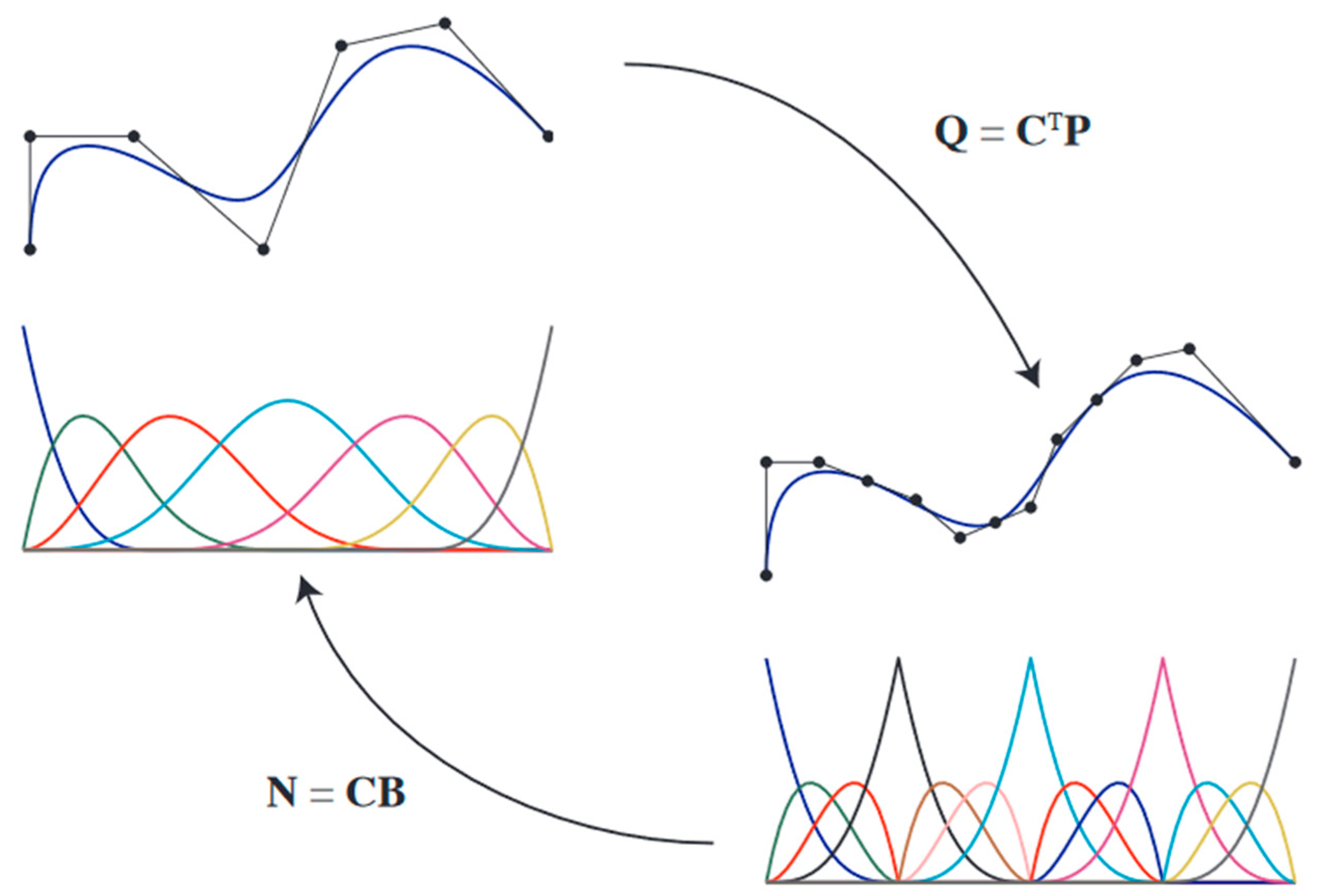
Like conventional finite detail analysis, the extracted Bezier factors of T-Splines are described as shown in Figure 1. A set of constant phrases in a polynomial foundation feature are referred to as a Bernstein foundation. Bezier factors may be processed in an identical manner as applied to widespread finite detail computer programs using identical information processing tables. In fact, it is convenient that only the form feature subprogram requires a change, as all of the different components relevant to the application of finite detail remain identical. A by-product of the extraction method is a detail extraction operator. This operator identifies detail-stage topology facts and worldwide smoothing facts and represents the canonical processing of T-joints. T-joints, referred to as “placing nodes” in finite detail analysis, are an essential characteristic of T-Splines.
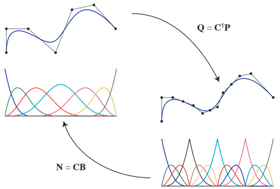
Figure 1.
See [31] for a Bézier extraction diagram of the B-Spline curve. The basic capabilities and control points of the B-Spline are denoted as N and P, respectively. The Bernstein polynomial and the control points are denoted as B and Q, respectively.
The idea of Bezier extraction is to reduce the number of control points while respecting the geometry without modifying the domain we would like to study. Further, Bezier extraction applies a local refinement to some parts of the domain (in which there will be major displacements). This technique improves the resolution of the FEM and generates precise results since the number of degrees of freedom is reduced. Note that the geometry must not change when inserting nodes.
Bezier extraction is fundamentally based on knot insertion, which will be briefly outlined for the univariate case below. A new knot can be inserted into the open node vector, resulting in the modified knot vector , and is the number of the basis function of order , where p < i < n + 1.
This insertion produces a new set of basis functions. To preserve the geometry or approximation while altering the parametrization of the basis, new control point values, , must be calculated from the original control points, , according to
If we are able to convert the T-Spline basis functions of N to Bernstein polynomials B, this permits the replacement of the T-Spline surface with a series of Bézier patches utilizing the conventional parametric domain. According to the Cox–de Boor formula, this can be expressed as follows.
The new set of so-called Bézier control points is computed from B-Spline control points, resulting in the following: . In remembering that the geometry must remain unchanged during the insertion of the nodes,
where is the coordinate in the standard domain of an individual Bézier patch, and is a T-Spline vector of the basis functions that are non-zero over the Bézier surface. However, is a vector of the tensor product of the basis functions of Bernstein polynomials associated with the Bézier surface. is the extraction operator.
For each localized T-Spline over an element, it can be explained as a linear combination of these Bernstein polynomials. In fact, there exists a coefficient , such that , where the convention is typical in finite element analysis, is the degree of the Bernstein polynomial, and is the dimension of the domain; for example, for the surfaces, .
We propose that univariate Bernstein polynomials form the basis of the Bézier surface, which are defined over the biunit interval [−1, 1], =, with , and : binomial coefficient.
We can define the multivariate Bernstein basis functions of degree as , with representing a pair of variables, and is a mapping from a pair of indices (i,j) to a single index. .
The calculation of the element extraction operators is conducted function-by-function, each basis function adding a line to each extraction operator corresponding to the Bézier elements in its support.
In 3D cases, the T-Spline volume in the parametric domain can be defined as follows:
Weights are scalar weights associated with each control point and T-Spline basis functions corresponding to control point :
2.2. Incorporating Bézier Extraction of T-Splines into Finite Element Method
The Bezier extraction of T-Splines produces a fixed set of Bezier elements (defined using Bernstein terminology) and the corresponding element extraction operators C and IEN (index element node) arrays. This shape is equivalent to that derived for NURBSs in [31] and can be incorporated into the finite detail components in a similar way. We construct the functional subspace of finite dim from the T-Spline functions, forming the specified geometry. From problem (14), the approximate problem is written as follows: given find such that :
where = , = , and is a bilinear form that often arises from integrating the product of the derivatives of the trial function and the test function over the domain. represents the right-hand side of the weak formulation.
With these combinations, problem (14) can be written in the form of a matrix problem:
We proceed as in the case of classical finite elements, with the global stiffness matrix A and the force vector F, which can be produced by performing an integration of the Bézier elements.
On each Bézier element, , we have , such as in the following: , where the elementary stiffness matrix and the vector force are assembled in the global matrix A and the vector F, respectively.
By taking into consideration the non-homogeneous Dirichlet boundary conditions and with the insertion of the Lagrange parameter, we obtain the following matrix problem that we wish to solve: =.
We use the element extraction operators, and the T-Spline function is defined as follows:
where , and represents the weight vector corresponding to the T-Spline control points. is the diagonal matrix form of vector .
We calculate the derivatives of the T-Splines with respect to the coordinates of the physical domain :
The approximation of the Bezier element is defined using a transformation to a reference element, which is the e The Jacobian determinant is defined as .
To solve linear system (18), we must calculate the elements of the rigidity matrix corresponding to any Bezier element in order to assemble them in a global matrix.
such as:
is the unit vector directed toward the outside of the domain, with the vector written as follows:
The matrix transforms the surface of the lateral domain to the reference surface .
To calculate all the elements of matrices, we use Gaussian quadrature.
2.3. Theoretically Stress Lateral Loading
The FEM analysis results are confirmed via comparison with the theoretically predicted tensile stress results and are presented according to the following equation [32,33]:
with
- ;
- P: the concentered load (N);
- X: the impact position;
- S: the section modulus of a circular hollow section;
- : the outer diameter;
- : the inner diameters of the pipe.
2.4. Mechanical Failure Criteria
In the literature, several failure criteria can be found that are used to analyze the performance of structures. The von Mises stress criterion is more commonly used in the field of linear elasticity to determine whether failure will occur by comparing the failure limits of materials. Due to this criterion, it is possible to know whether the structure under study can function normally under load. The equation is expressed as follows:
where , , and are the first, second, and third principal stresses.
3. Computational Modeling and Simulation
This section explains the steps used to model a 3D cylindrical shell pipe subjected to a concentrated and compressive load using the classic finite element method based on Abaqus/CAE and the IGA approach based on the NURBS and the T-Spline methods.
3.1. Cylindrical Shell 3D Pipe Geometry
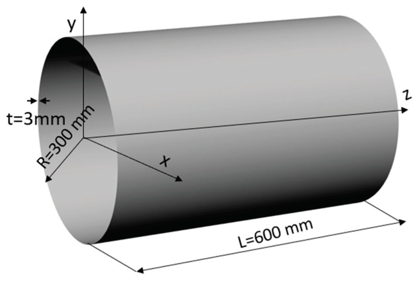
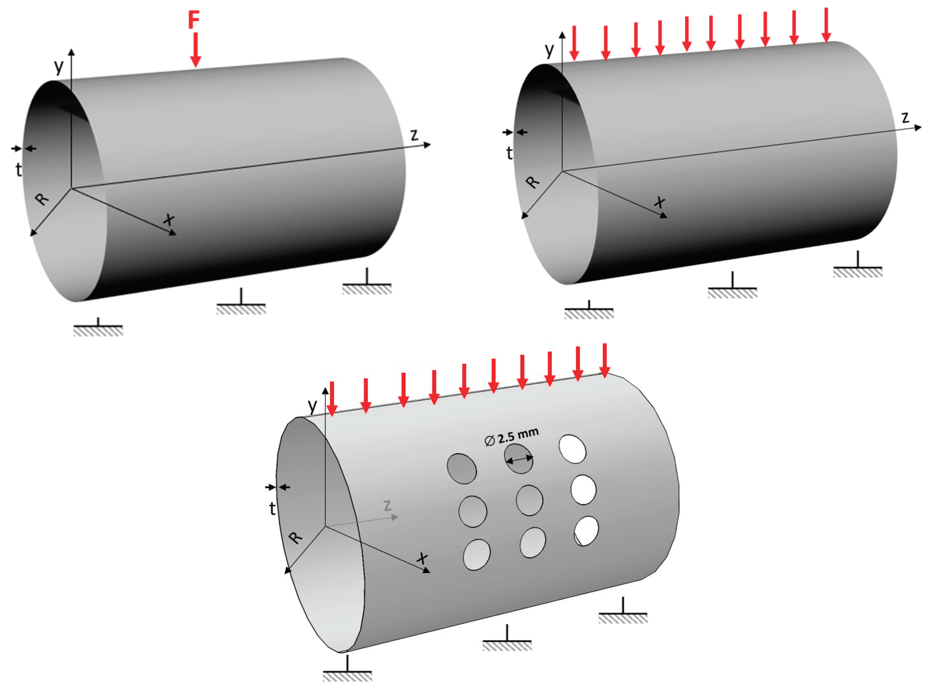
The geometry of the 3D cylindrical shell pipe studied is shown in Figure 2.
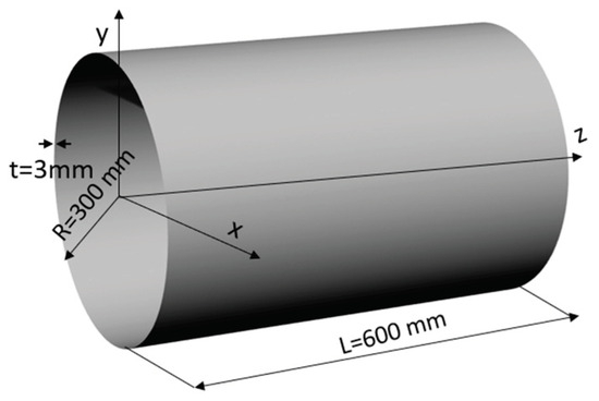
Figure 2.
The geometry of the 3D cylindrical shell pipe.
3.2. Material
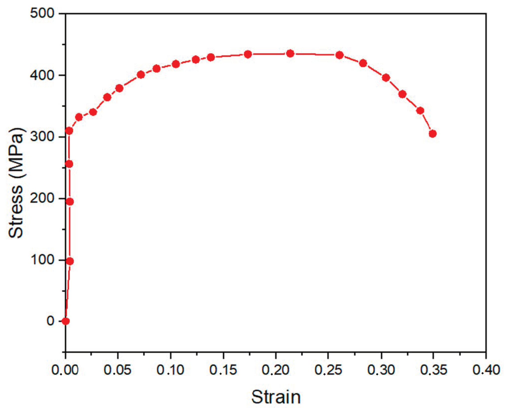
P264GH steel material [34] (Table 1) was used in this study. The stress–strain curve of the mechanical test is shown in Figure 3. The behavior of this material follows the Ramberg–Osgood law, which is described as follows:
where

Table 1.
Mechanical properties of P264GH steel.

Figure 3.
Stress–strain curve of P264GH steel.
The stress–strain curve of the P264GH steel is illustrated in Figure 3:
3.3. Meshing, Loadings, and Boundary Conditions
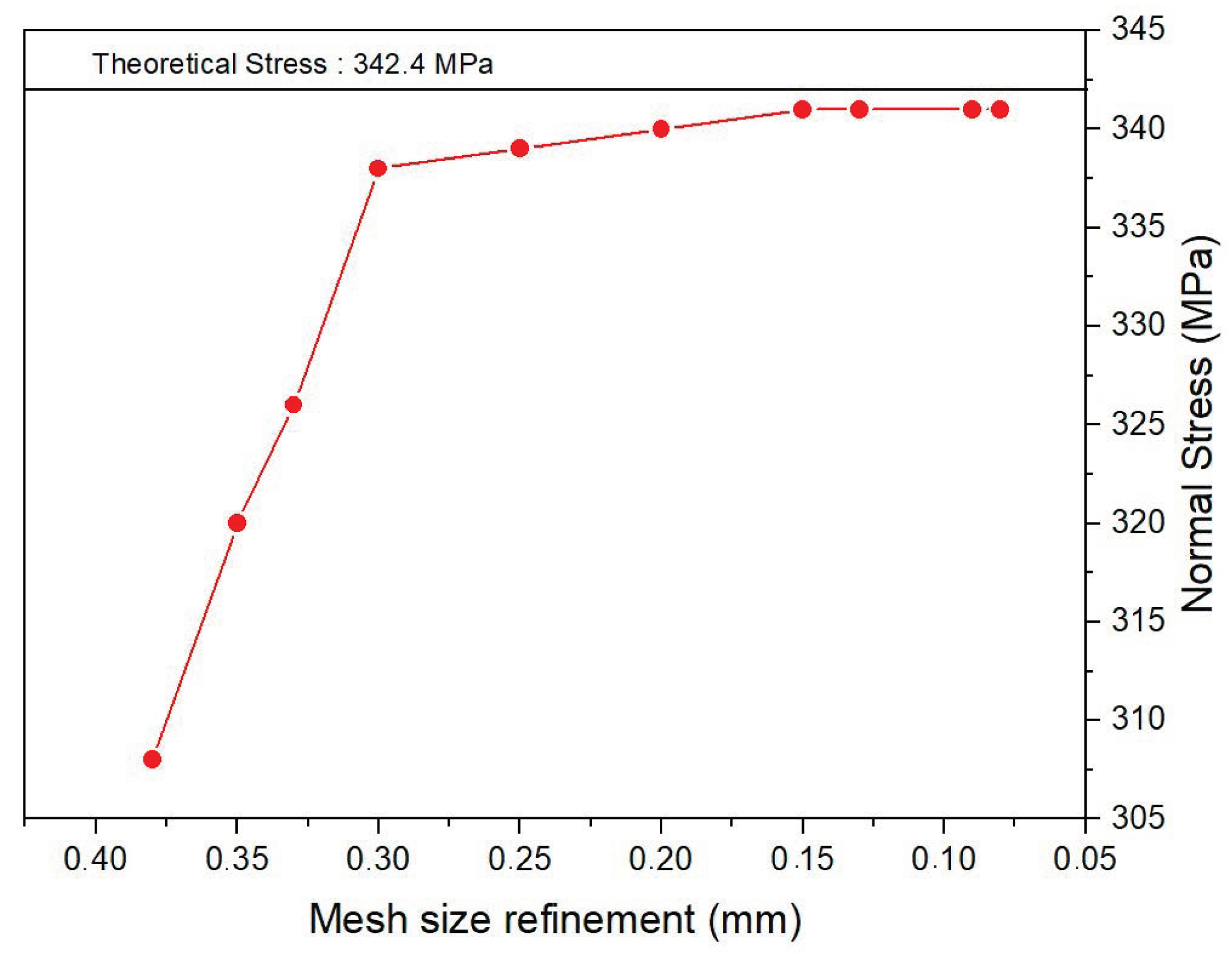
To ensure a robust convergence of results in Abaqus/CAE and facilitate pertinent comparisons with the IGA approach based on the NURBS and T-Spline results, we performed a mesh convergence study for the proposed refinements. We established that a mesh size ranging from 0.15 mm to 0.09 mm for the calculation of stress is robust and consistent (Figure 4). Additionally, for an efficient computation time ratio, we used a mesh size of 0.15 mm for this investigation.
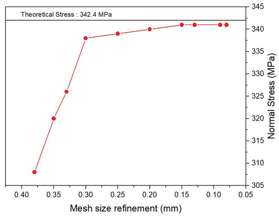
Figure 4.
Mesh size convergence (finite element method (FEM) Abaqus/computer-aided engineering (CAE)).
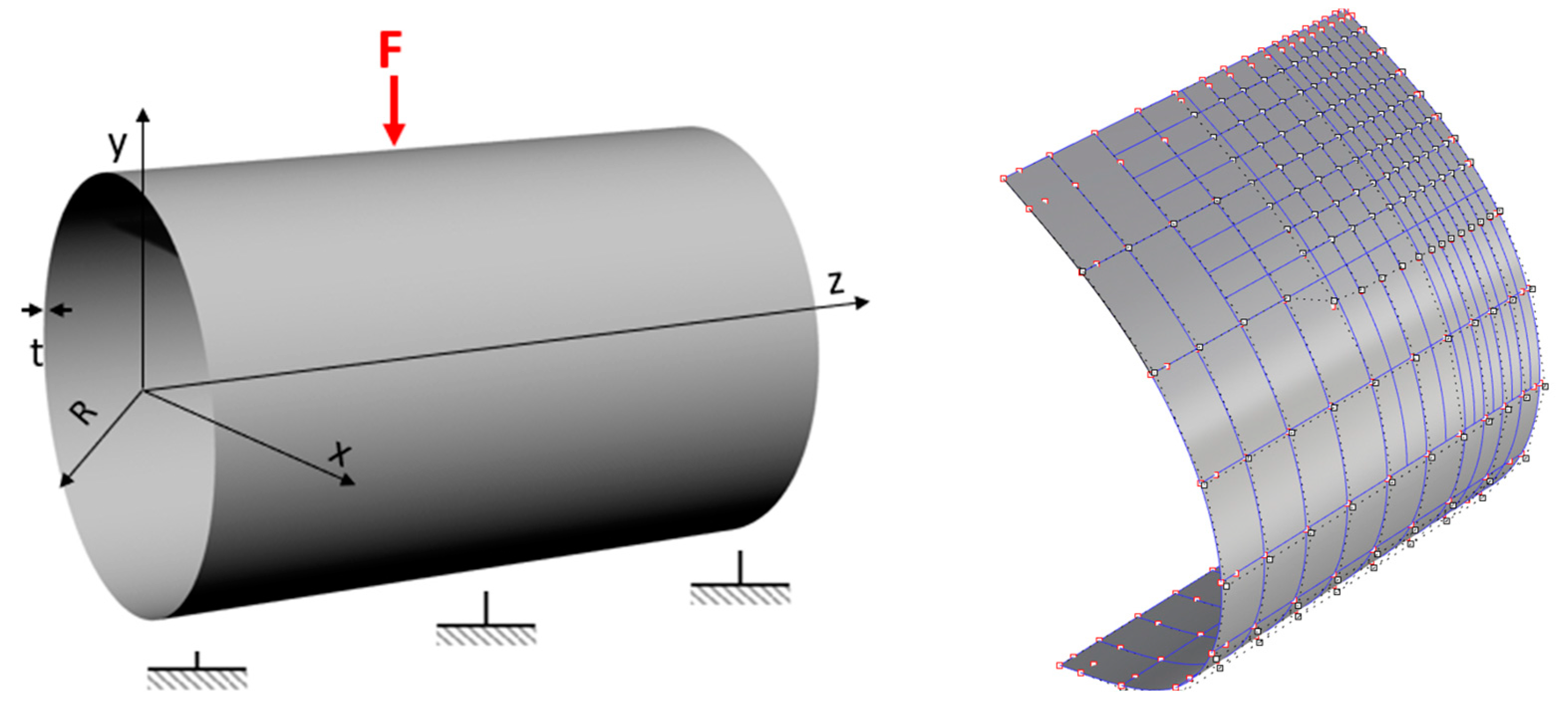
In this study, we employed the IGA approach based on the T-Spline method to resolve industrial mechanical issues, particularly the failure of pipelines due to the side impact of excavation machines during installation, pipe–soil interactions, and preformed holes. The impact was modeled using an applied load (F) and a line compression load (Figure 5). It is important to note that this investigation was carried out in the linear elasticity domain.
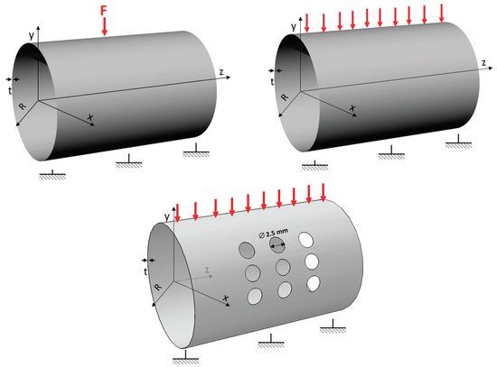
Figure 5.
The geometry and loading conditions of the cylindrical shell pipe.
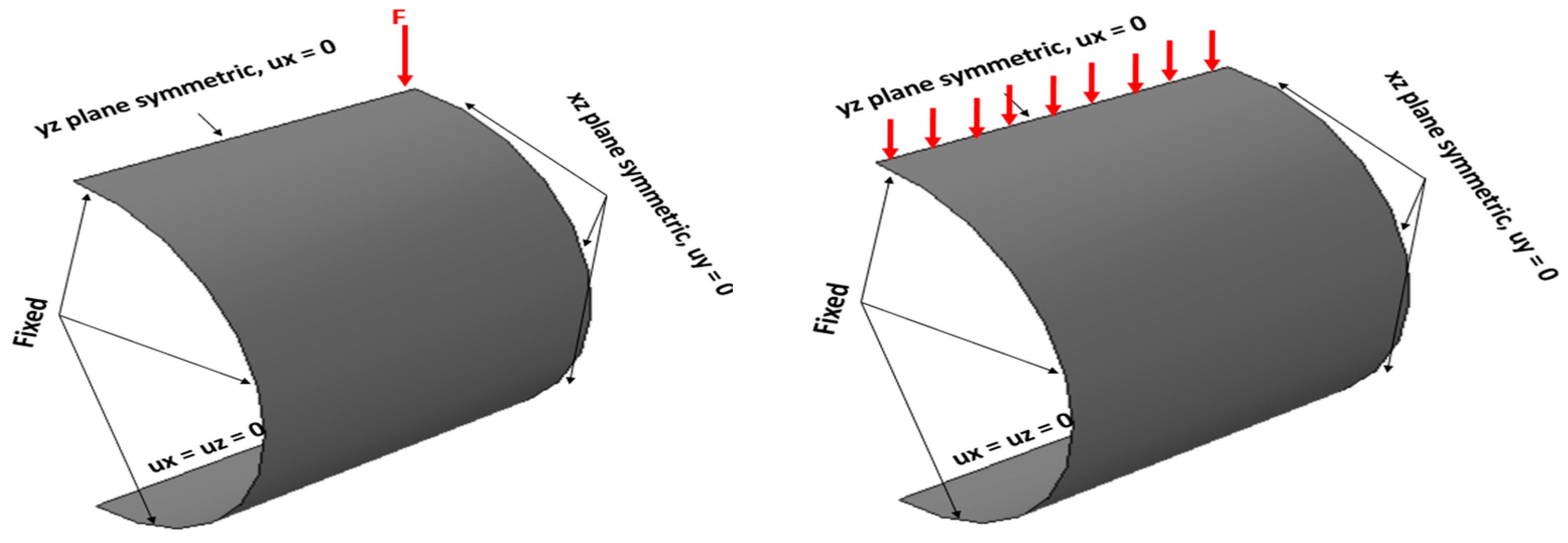
Considering geometric symmetry and to enable an efficient computation time ratio, we used half of a 3D cylindrical shell pipe (Figure 6) to model the impact for both numerical investigation methods, the finite element method (FEM) according to Abaqus/CAE and the IGA approach based on NURBSs and T-Splines.

Figure 6.
The boundary conditions for half of a cylindrical shell pipe.
After obtaining the efficient convergence of the numerical results in Abaqus/CAE, we locally refined the mesh where we applied the load, as shown in Figure 7. We used linear quadrilateral elements of type S4 to model the 3D cylindrical shell pipe case. This element is characterized by good computational time savings, is easier to mesh, and is less prone to negative Jacobian errors than 3D solid elements.

Figure 7.
Mesh FEM (Abaqus/CAE); total number of nodes: 1197; total number of elements: 1176.
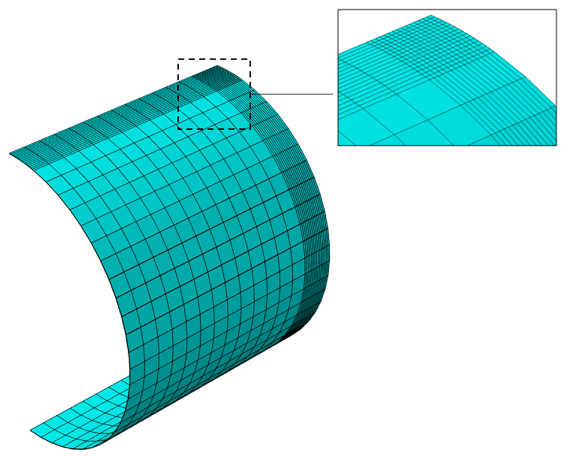
In the IGA approach, we used an exact mesh generated using NURBS functions (Figure 9a), and we took advantage of Bézier extraction for the T-Spline surfaces (Figure 8). Contrary to NURBS functions, T-Splines enable local adjustments by introducing additional control points only in areas where higher resolution is required (Figure 9d). This feature enhances the efficiency of capturing details during analysis.

Figure 8.
T-Spline surface with 112 control points and 88 T mesh elements.
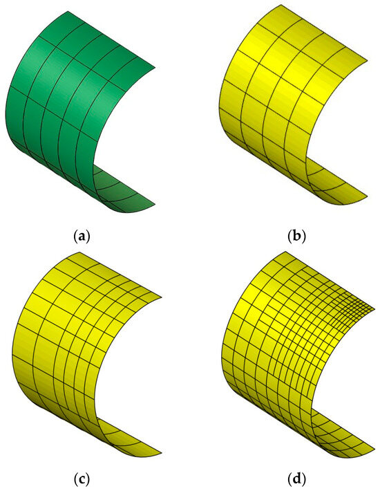
Figure 9.
The demi-cylinder with 15 Non-Uniform Rational B-Spline (NURBS) mesh elements and 32, 50, and 215 T mesh elements.
4. Numerical Results and Discussion
In this section, three numerical evaluations are introduced to highlight the primary advantages of employing the T-Spline approach for isogeometric analysis relating to 3D cylindrical shell pipe mechanical computation issues. Firstly, a 3D cylindrical shell pipe subjected to concentered elastic load and compressive load benchmarks was analyzed to verify the capability of the adaptive T-Spline approach for isogeometric analysis and to study the robustness of the 3D mechanical cylindrical shell pipe. The obtained results were compared and validated with results found in the literature, particularly those concerning the use of NURBS IGA and FEM Abaqus/CAE methods. In the final analysis, we will evaluate a 3D cylindrical shell involving the preformed hole issue. The goal is to provide further analysis evaluating the performance and robustness of T-Splines for the computational modeling of trimmed surfaces.
4.1. Cylindrical Shell 3D Pipe under Concentrated Load
We will study a cylindrical shell pipe without internal pressure subjected to compressive load in order to model impact machine excavation.
We performed a comparative study of the computation time between the different methods used in this investigation. The results show that the computation time (Table 2) of IGA based on the T-Spline method is shorter than that of IGA based on NURBS and FEM Abaqus/CAE. This confirms the results of Du et al. [20] and Guo et al. [35]. The better computation time of the T-Spline method is due to the use of fewer control points (Figure 10) compared to the NURBS method. Furthermore, T-Splines combine the advantages of NURBSs and polygonal modeling techniques, leading to better convergence of the results.
Table 2.
Time calculation comparison for FEM, IGA NURBS, and IGA T-Splines carried out using Intel® Core ™ i5-8250U CPU 1.60 GHz (4 CPUs).

Figure 10.
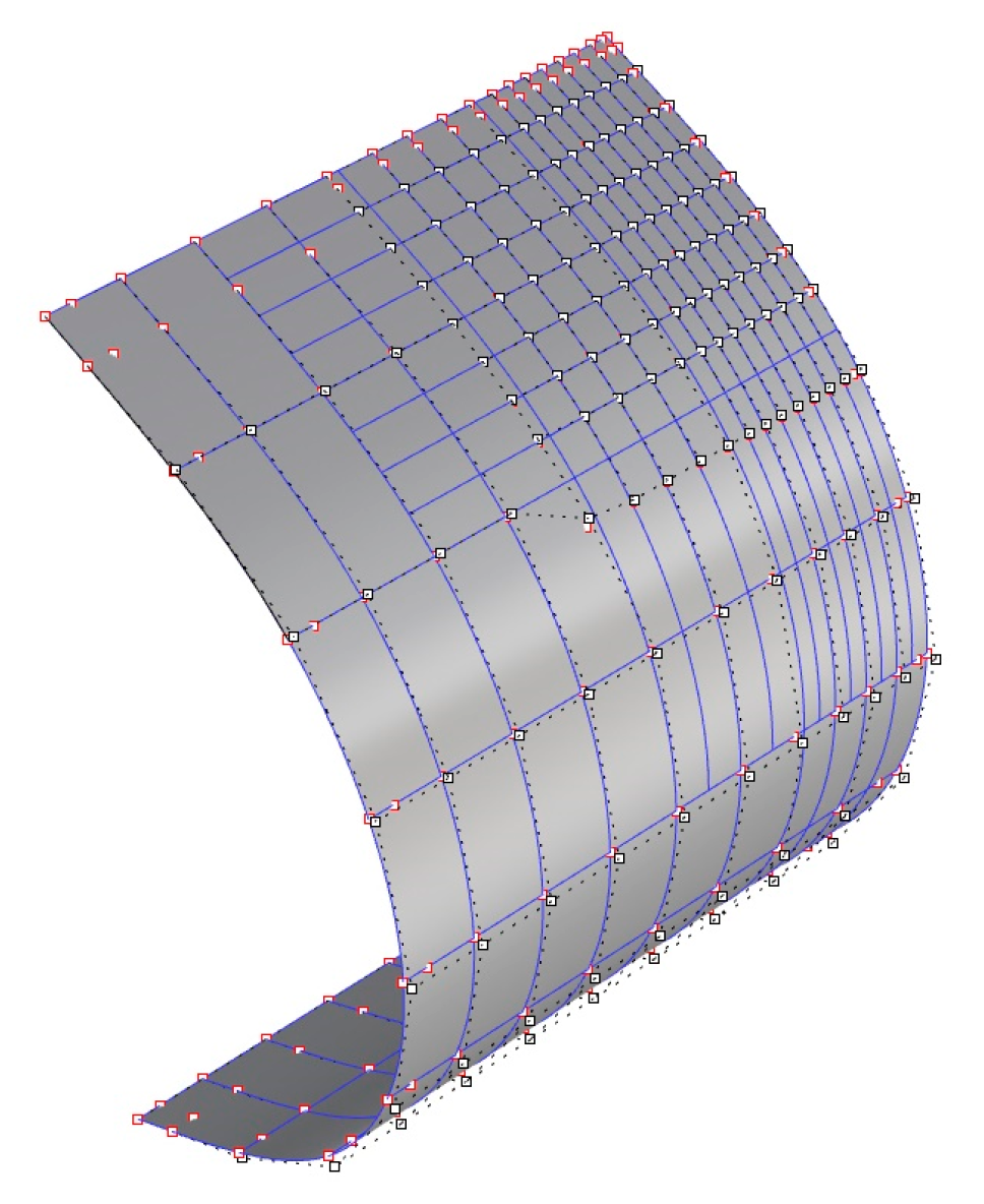
Boundary conditions and T-Spline surface with 326 control points and 215 T mesh elements.
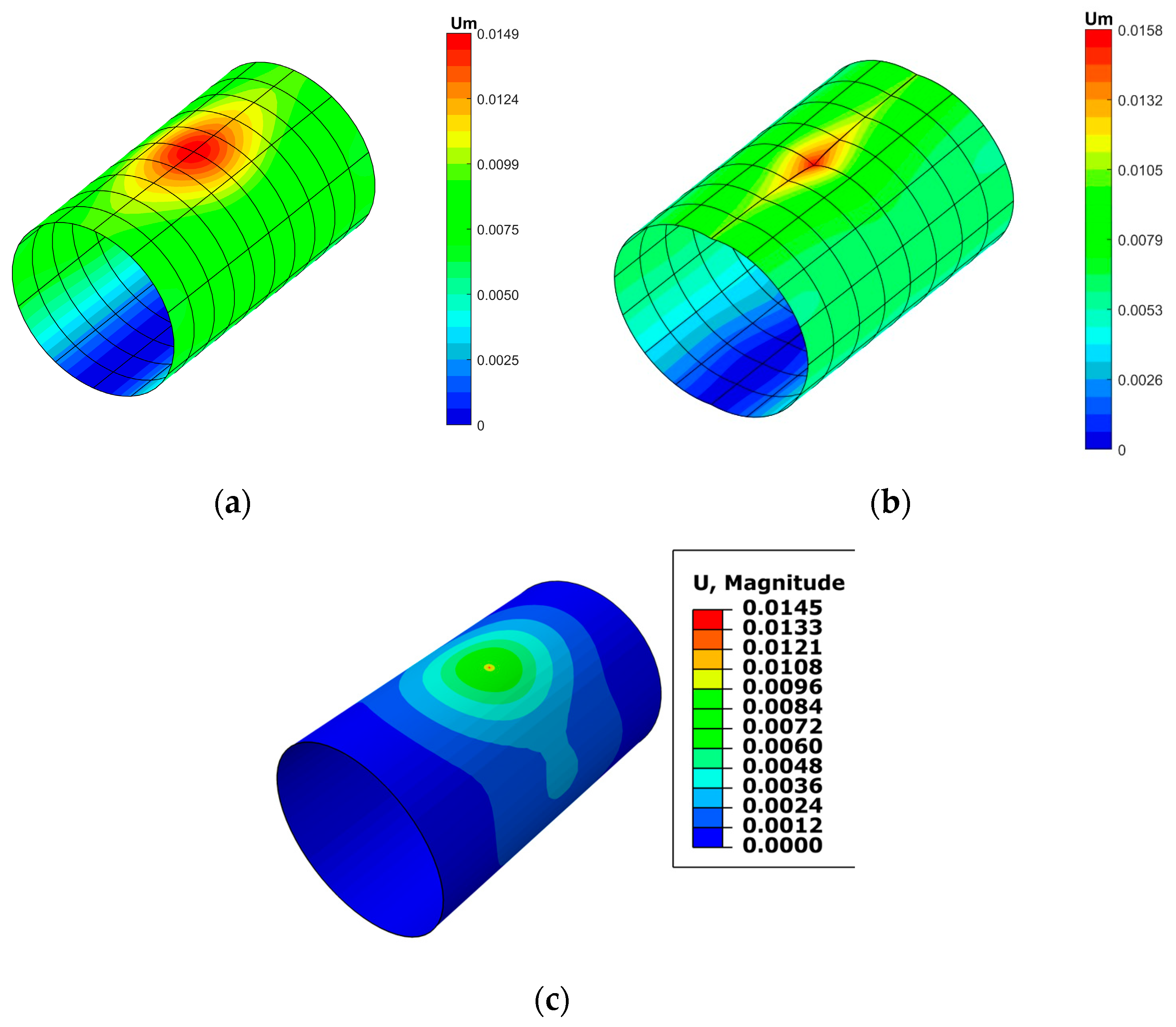
Figure 11 illustrates a comparison of the displacement magnitude of a 3D cylindrical shell pipe subjected to a force of 1.6 kN computed using the FEM (Abaqus/CAE) (), IGA NURBS (), and IGA T-Spline () methods. The results show that the IGA T-Spline method yields better results than the IGA NURBS method, which is also a robust method. These results lead to the same conclusion reached by Du et al. [21]. The disparity between the T-Spline and NURBS methods is that the IGA approach based on T-Splines provides a high level of flexibility in 3D surface shaping, and T-Splines allow for the local refinement of the mesh (Figure 12). T-Splines are often used in conjunction with subdivision surfaces. This combination allows for the creation of highly detailed models with smooth surfaces.

Figure 11.
Displacement magnitude of 3D cylinder pipe: (a) result of NURBS; (b) result of T-Splines; (c) result of Abaqus/CAE finite element analysis (FEA).
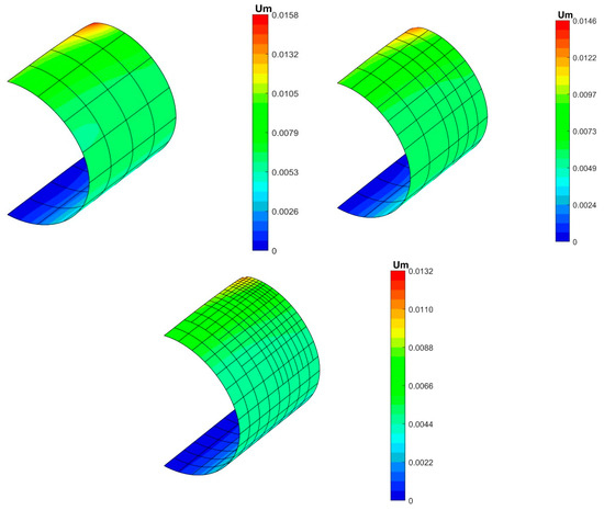
Figure 12.
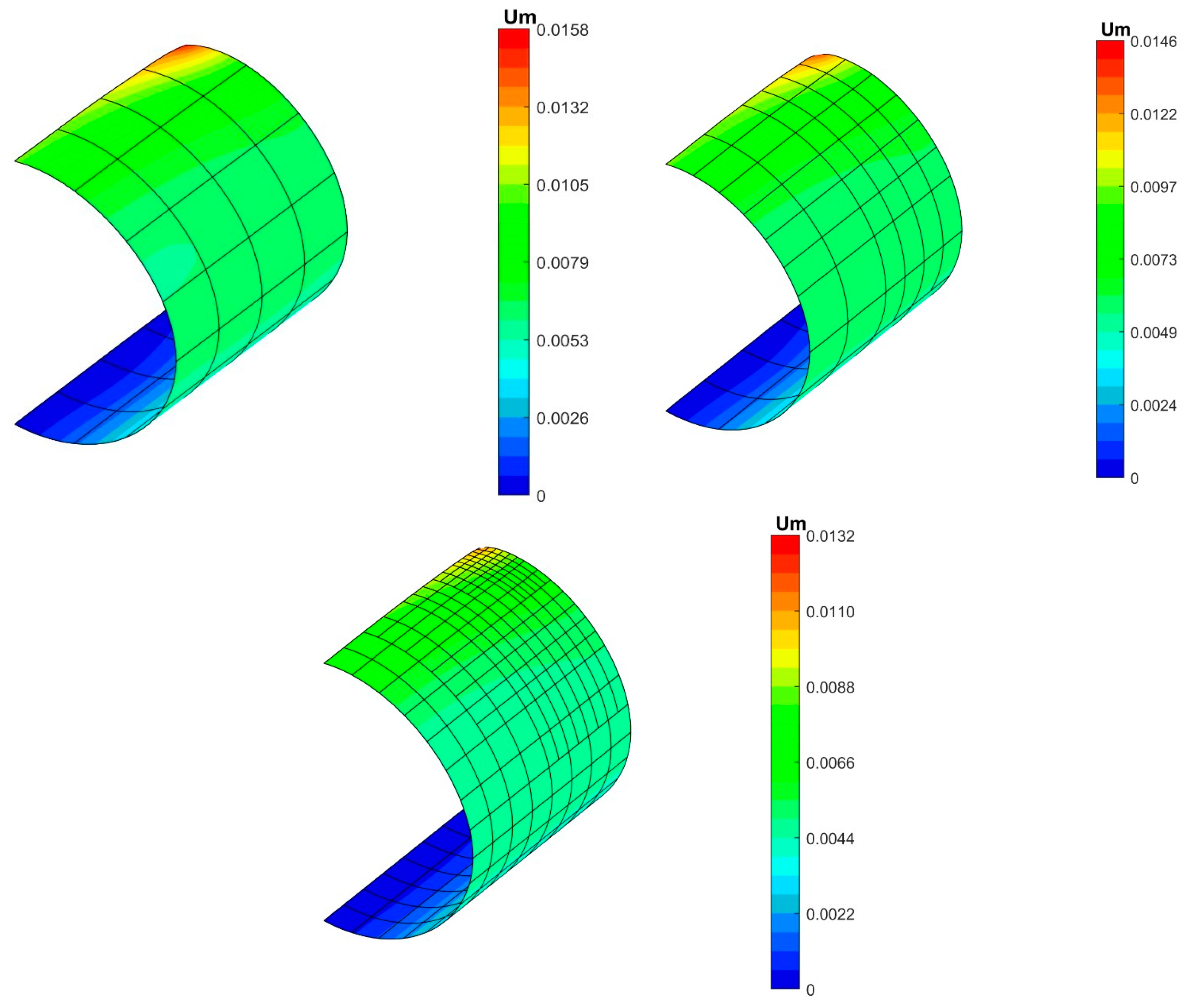
The displacement magnitude results for a 3D cylindrical pipe for various mesh refinements of 32, 50, and 215 T-Spline elements using the Bézier extraction method.
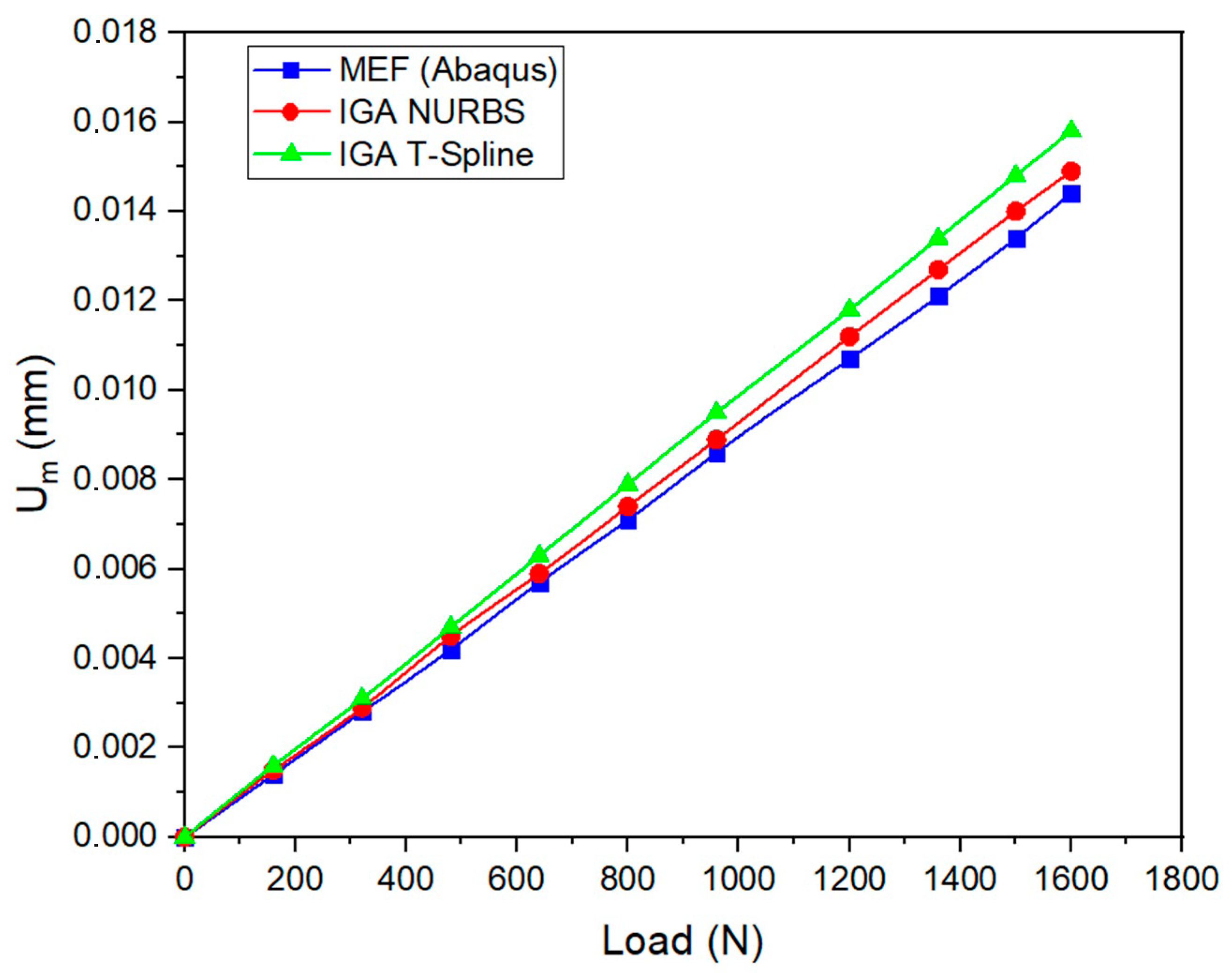
To complete the previously highlighted results and apply them to the study of the mechanical behavior and strength of a 3D pipe, we analyzed the load variation applied to the 3D cylindrical shell pipe as a function of displacement using the different FEM Abaqus/CAE, IGA NURBS, and T-Spline methods, as illustrated in Figure 13. Load magnitudes varying from 0 N to 1600 N were used to maintain linear elasticity and predict the impact of the excavator during work not subjected to internal pressure. The results show linearity between the load and displacement curves. Furthermore, it is important to point out that, after 1200 N, there is some variation in the results between the three methods. The divergence of the numerical results is explained by the influence of the proximity of the plastic zone.
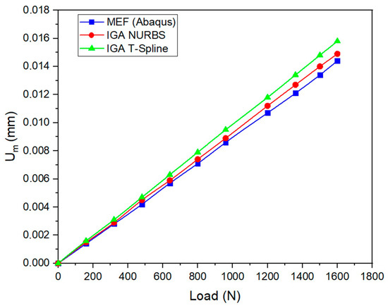
Figure 13.
Load–displacement curves of the 3D cylindrical shell pipe.
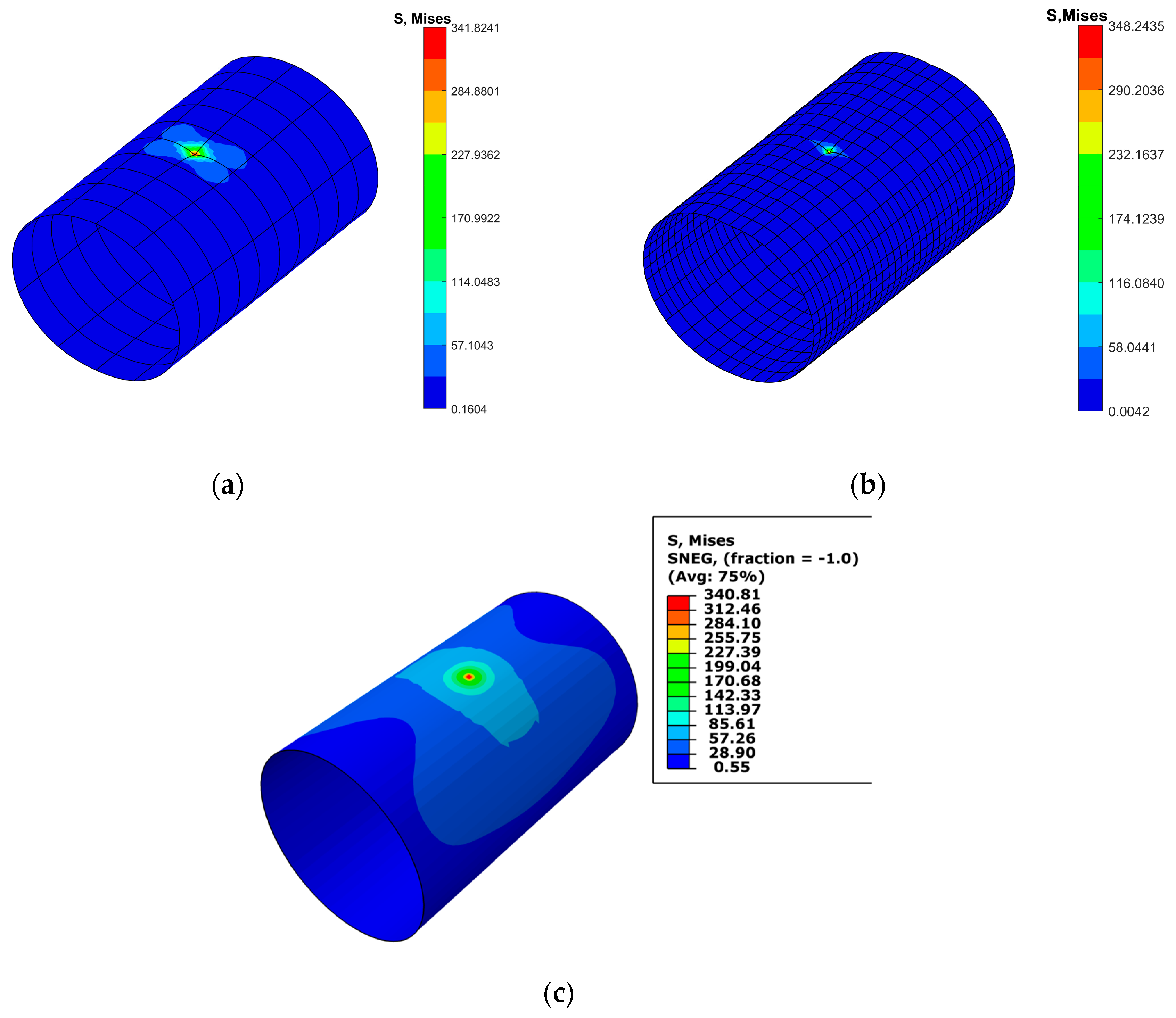
Figure 14 illustrates the von Mises stress distribution around an applied radial load of 1.6 kN. Evaluations were performed for two numerical references methods, FEM Abaqus/CAE, IGA NURB and IGA T-Splines. The results confirm that the IGA approach based on the T-Spline method is successful compared to the numerical references methods. We conclude that, thanks to the T-Spline method, we obtain higher values of around the impact region than those found using FEM Abaqus/CAE () and IGA NURBS (). The value found using the T-Splines method is in close proximity to the yield strength of the material. This allows us to provide pertinent information on fracture prediction and the robust convergence of the results that were undetected when using the FEM Abaqus/CAE and IGA NURBS methods. The robustness of the T-Spline method relates to its capability to introduce local control points, allowing for more detailed information to be obtained in certain regions without compromising the overall simplicity of the model. The local refinement feature of T-Splines is particularly useful for efficiently capturing geometric details in specific areas of a model.

Figure 14.
von Mises stress of 3D cylindrical pipe: (a) result of NURBS; (b) result of T-Splines; (c) result of Abaqus/CAE FEA.
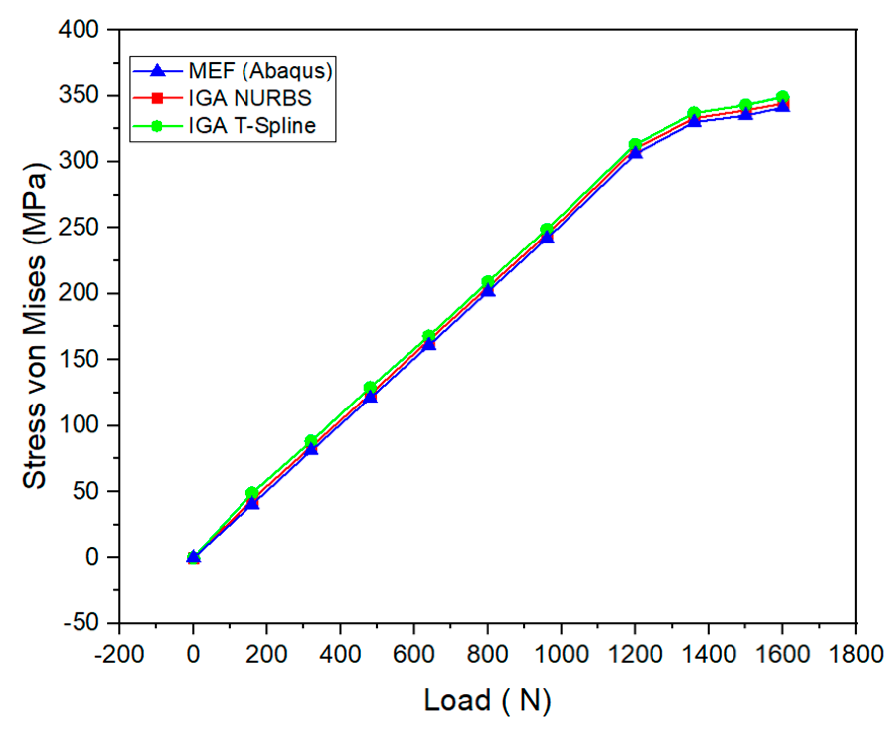
On the other hand, we evaluated the structural integrity of the 3D cylindrical shell pipe by applying various load values (from 0 N to 1600 N). We extracted different maximum values (denoted as 348 MPa) of the von Mises stress around the force impact region for various methods, especially using FEM Abaqus/CAE, IGA NURBSs, and IGA T-Splines (Figure 15). The results indicate that the stress curves converge closely with minor disparity. The value of 348 MPa obtained through the use of IGA T-Splines is higher than that of FEM Abaqus/CAE and IGA NURBSs.
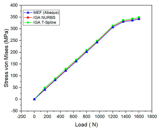
Figure 15.
Load–von Mises stress curves of the 3D cylindrical shell pipe.
In addition, it was observed that the curve diverges from linearity when it exceeds the value of 340 MPa above 1200 N, suggesting a transition to the plastic region. This nonlinearity in the curve indicates a change in material behavior and signifies that the structural response is moving beyond the linear elastic domain.
4.2. Cylindrical 3D Shell Pipe under Compressive Loading
We studied a cylindrical shell pipe subjected to compressive load, modeling the pipe–soil interaction. The predicted load of this interaction between the pipe and the soil is 1.9 kN (Figure 16).
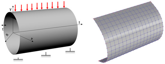
Figure 16.
Boundary conditions and T-Spline surface with 361 control points and 256 T mesh elements.
T-Splines enable the addition of some local refinement control points in the area where good convergence is required (Figure 17), which is not available in IGA based on NURBS functions.
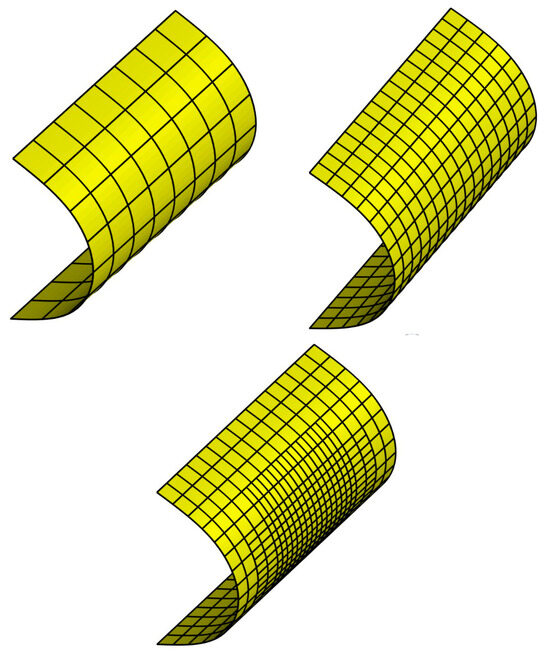
Figure 17.
Mesh extraction Bézier of semi-cylinder with 64, 256, and 376 T mesh elements.
We compared the results found using T-Splines for different proposals for the local refinement of control points in a 3D cylinder (Figure 18). The obtained results show a dependence on the number of refinement control points. With 122 control points, the maximum displacement on the cylinder is 0.0728 mm, and when we refine up to 361 control points, the maximum displacement on the cylinder is reduced to 0.0693 mm.
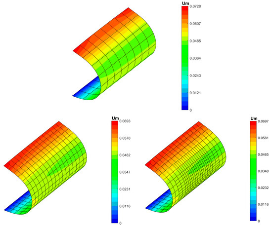
Figure 18.
The displacement magnitude results of a 3D cylindrical pipe for various mesh refinements using the T-Spline method.
Further, we performed a comparative study using a T-Spline for comparison and validation with results found in the literature, especially those relating to the use of the NURBS IGA and FEM Abaqus/CAE methods (Figure 19). The amount of displacement calculated using the T-Spline method is 0.0728 mm, which is slightly higher than that found when using IGA NURBSs and FEM Abaqus at 0.0531 mm and 0.0626 mm, respectively. Note that in T-Splines with 361 control points, the maximum displacement per cylinder is reduced to 0.0693 mm. We conclude from all these results that we are confident in using the T-Spline method as an alternative method to investigate the mechanical performance of cylindrical shell structures.
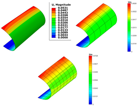
Figure 19.
The displacement magnitude results of a 3D cylinder pipe for FEM Abaqus/CAE, IGA NURBSs, and T-Splines.
4.3. Three-Dimensional Cylindrical Shell Pipe with Preformed Holes and Pipe Junction under Compressive Loading
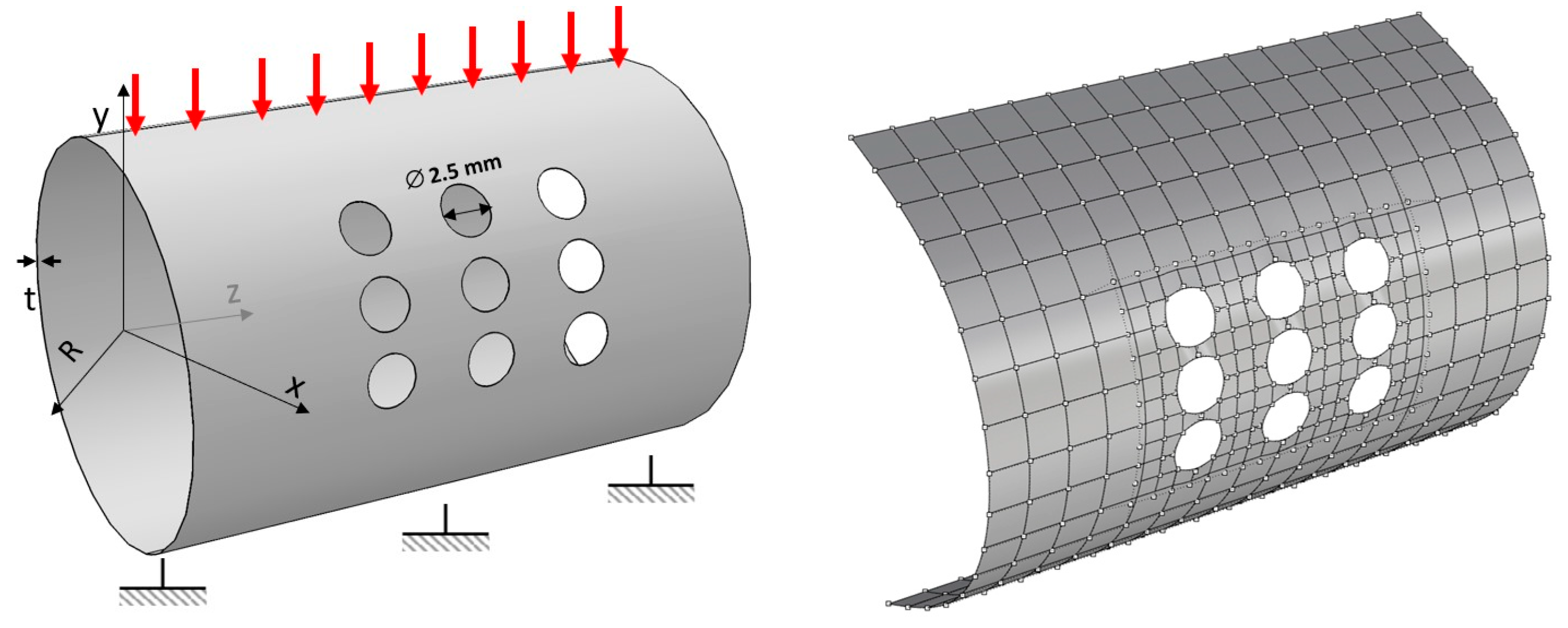
In this section, we evaluated a 3D cylindrical shell pipe with a preformed hole under a compressive load (Figure 20) in relation to structural engineering problems. The objective is to evaluate the efficiency and robustness of the T-Spline method in the field of trimmed surfaces. In this study, we compared the results found when using the T-Spline method with the Abaqus/CAE finite element method because IGA based on NUBRSs is too limited for the evaluation of the trimmed surfaces; it requires a specific adjustment of the interpolation domain, especially the B-Spline or NUBRS interpolation functions, when considering a trimmed geometry. A 3D cylindrical shell pipe (r = 300 mm; L = 600 mm; thickness = 3 mm) with nine holes with a 2.5 mm diameter was evaluated with the objective of assessing the mechanical robustness and structural integrity of pipes with preformed holes in cases of severe mechanical and chemical damage. This recent investigation completes the research conducted in [36,37,38].

Figure 20.
Boundary condition and T-Spline surface with 485 control points and 340 T mesh elements.
In Figure 21, we compare the numerical results of the displacement between the T-Spline and FEM Abaqus methods, and in noting that the NURBS IGA method is very limited in terms of studying trimmed surfaces, it was not considered for comparison in this study. The maximum displacement value was found to be higher than the FEM Abaqus displacement value , and we concluded that, in the case of preformed holes, the displacement value increased by ; this suggests the performance degradation of a cylindrical shell pipe with preformed holes, leading to integrity issues.
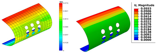
Figure 21.
The displacement magnitude results of a 3D cylindrical pipe with holes calculated using the T-Spline method.
In addition, the T-Spline method once again shows its power and capability in terms of computing trimmed and untrimmed surfaces.
5. Conclusions
An investigation of the mechanical performance of a 3D cylindrical shell pipe with and without preformed holes under concentrated and compressive loading in terms of the linear elastic behavior in the cases of trimmed and untrimmed surfaces using the IGA method based on the T-Spline technique was successfully conducted. The numerical results obtained, especially relating to displacement and von Mises stress, were compared and validated with results found in the literature, particularly concerning the NURBS IGA and FEM Abaqus methods. The results show that the computation time of IGA based on T-Splines is shorter than the IGA NURBS and FEM Abaqus/CAE methods. Moreover, the results confirm that the IGA approach based on the T-Spline method shows successful achievements compared to numerical references found in the literature review.
The numerical results of von Mises stress found, through the use of the T-Spline method, are in close proximity to the yield strength of the material. This allows us to provide pertinent information on fracture prediction and the robust convergence of the results that were undetected when using the FEM Abaqus/CAE and the IGA NURBS methods. The robustness of the T-Spline method is based on its ability to introduce local control points in the area where robust convergence is required, which is too limited in IGA based on NURBS functions. In addition, through the use of T-Splines, we will end up with a linear system with a slightly lower degree of freedom with a stiffness matrix that is less full compared to the one obtained when using the NURBS method. This makes it easy to invert this matrix with a fairly small inversion error.
On the other hand, a 3D cylindrical shell pipe with a preformed hole under compressive load was studied as a structural engineering problem with the objective of evaluating the efficiency and robustness of the T-Spline method in the field of trimmed surfaces. We noticed that the NURBS IGA method is very limited when evaluating trimmed surfaces. The maximum displacement value was found to be higher than the FEM Abaqus displacement value; thus, we conclude that, in the case of preformed holes, the displacement value increased, which suggests the performance degradation of a cylindrical shell pipe with preformed holes, leading to integrity issues.
Future research work will involve the integration of a complementary investigation on the impact of machine excavation on pipes under internal pressure. This study will consider scenarios both with and without the presence of cracks using the IGA approach based on T-Splines. The aim is to evaluate the mechanical behavior and performance of cylindrical shell pipelines, addressing problems in both linear elastic and dynamic studies.
Author Contributions
Conceptualization, S.E.F., O.K. and A.E.; methodology, S.E.F., O.K. and A.E.; software, S.E.F., O.K. and A.E.; validation, S.E.F., O.K., A.E., S.V. and M.M.; formal analysis S.E.F., O.K., A.E., S.V. and M.M.; investigation, S.E.F., O.K. and A.E.; resources, A.E.; data curation, S.E.F., O.K. and A.E.; writing—original draft preparation, S.E.F., O.K., A.E., S.V. and M.M.; writing—review and editing, A.E. and S.V.; visualization, S.E.F., O.K., A.E., S.V. and M.M.; supervision, S.E.F., O.K., A.E., S.V. and M.M.; project administration, A.E.; funding acquisition, A.E., S.V. and M.M. All authors have read and agreed to the published version of the manuscript.
Funding
This research received no external funding.
Data Availability Statement
Data are contained within this article.
Conflicts of Interest
The authors declare no conflicts of interest.
References
- Bazilevs, Y.; Calo, V.; Cottrell, J.; Evans, J.; Hughes, T.; Lipton, S.; Scott, M.; Sederberg, T. Isogeometric analysis using T-splines. Comput. Methods Appl. Mech. Eng. 2010, 199, 229–263. [Google Scholar] [CrossRef]
- Cottrell, J.A.; Hughes, T.J.R.; Bazilevs, Y. Isogeometric Analysis: Toward Integration of CAD and FEA, 1st ed.; Wiley: Hoboken, NJ, USA, 2009. [Google Scholar]
- Scutaru, M.L.; Guendaoui, S.; Koubaiti, O.; El Ouadefli, L.; El Akkad, A.; Elkhalfi, A.; Vlase, S. Flow of Newtonian Incompressible Fluids in Square Media: Isogeometric vs. Standard Finite Element Method. Mathematics 2023, 11, 3702. [Google Scholar] [CrossRef]
- Oesterle, B.; Geiger, F.; Forster, D.; Fröhlich, M.; Bischoff, M. A study on the approximation power of NURBS and the significance of exact geometry in isogeometric pre-buckling analyses of shells. Comput. Methods Appl. Mech. Eng. 2022, 397, 115144. [Google Scholar] [CrossRef]
- Koubaiti, O.; Elkhalfi, A.; El-Mekkaoui, J. WEB-Spline Finite Elements for the Approximation of Navier-Lamé System with CA, B Boundary Condition. Abstr. Appl. Anal. 2020, 2020, 1–14. [Google Scholar] [CrossRef]
- Koubaiti, O.; El Fakkoussi, S.; El-Mekkaoui, J.; Moustachir, H.; Elkhalfi, A.; Pruncu, C.I. The treatment of constraints due to standard boundary conditions in the context of the mixed Web-spline finite element method. Eng. Comput. 2021, 38, 2937–2968. [Google Scholar] [CrossRef]
- Farahat, A.; Verhelst, H.M.; Kiendl, J.; Kapl, M. Isogeometric analysis for multi-patch structured Kirchhoff–Love shells. Comput. Methods Appl. Mech. Eng. 2023, 411, 116060. [Google Scholar] [CrossRef]
- Hattori, G.; Trevelyan, J.; Gourgiotis, P. An isogeometric boundary element formulation for stress concentration problems in couple stress elasticity. Comput. Methods Appl. Mech. Eng. 2023, 407, 115932. [Google Scholar] [CrossRef]
- Sederberg, T.W.; Cardon, D.L.; Finnigan, G.T.; North, N.S.; Zheng, J.; Lyche, T. T-spline Simplification and Local Refinement. ACM Trans. Graph. 2004, 23, 239–247. [Google Scholar] [CrossRef]
- Evans, E.; Scott, M.; Li, X.; Thomas, D. Hierarchical T-splines: Analysis-suitability, Bézier extraction, and application as an adaptive basis for isogeometric analysis. Comput. Methods Appl. Mech. Eng. 2015, 284, 1–20. [Google Scholar] [CrossRef]
- Wei, X.; Zhang, Y.; Liu, L.; Hughes, T.J. Truncated T-splines: Fundamentals and methods. Comput. Methods Appl. Mech. Eng. 2017, 316, 349–372. [Google Scholar] [CrossRef]
- Maier, R.; Morgenstern, P.; Takacs, T. Adaptive refinement for unstructured T-splines with linear complexity. Comput. Aided Geom. Des. 2022, 96, 102117. [Google Scholar] [CrossRef]
- Toshniwal, D. Quadratic splines on quad-tri meshes: Construction and an application to simulations on watertight reconstructions of trimmed surfaces. Comput. Methods Appl. Mech. Eng. 2022, 388, 114174. [Google Scholar] [CrossRef]
- Liu, Z.; Cheng, J.; Yang, M.; Yuan, P.; Qiu, C.; Gao, W.; Tan, J. Isogeometric analysis of large thin shell structures based on weak coupling of substructures with unstructured T-splines patches. Adv. Eng. Softw. 2019, 135, 102692. [Google Scholar] [CrossRef]
- Dörfel, M.R.; Jüttler, B.; Simeon, B. Adaptive isogeometric analysis by local h-refinement with T-splines. Comput. Methods Appl. Mech. Eng. 2010, 199, 264–275. [Google Scholar] [CrossRef]
- Fathi, F.; de Borst, R. Geometrically nonlinear extended isogeometric analysis for cohesive fracture with applications to delamination in composites. Finite Elem. Anal. Des. 2021, 191, 103527. [Google Scholar] [CrossRef]
- Zhuang, C.; Xiong, Z.; Ding, H. Bézier extraction based isogeometric topology optimization with a locally-adaptive smoothed density model. J. Comput. Phys. 2022, 467, 111469. [Google Scholar] [CrossRef]
- Coradello, L.; D’angella, D.; Carraturo, M.; Kiendl, J.; Kollmannsberger, S.; Rank, E.; Reali, A. Hierarchically refined isogeometric analysis of trimmed shells. Comput. Mech. 2020, 66, 431–447. [Google Scholar] [CrossRef]
- Reichle, M.; Arf, J.; Simeon, B.; Klinkel, S. Smooth multi-patch scaled boundary isogeometric analysis for Kirchhoff–Love shells. Meccanica 2023, 58, 1693–1716. [Google Scholar] [CrossRef]
- Du, X.; Zhao, G.; Wang, W.; Guo, M.; Zhang, R.; Yang, J. NLIGA: A MATLAB framework for nonlinear isogeometric analysis. Comput. Aided Geom. Des. 2020, 80, 101869. [Google Scholar] [CrossRef]
- Du, X.; Zhao, G.; Zhang, R.; Wang, W.; Yang, J. Numerical implementation for isogeometric analysis of thin-walled structures based on a Bézier extraction framework: NligaStruct. Thin-Walled Struct. 2022, 180, 109844. [Google Scholar] [CrossRef]
- Shan, X.; Yu, W.; Gong, J.; Wen, K.; Wang, H.; Ren, S.; Wei, S.; Wang, B.; Gao, G.; Zhang, G. A methodology to determine the target reliability of natural gas pipeline systems based on risk acceptance criteria of pipelines. J. Pipeline Sci. Eng. 2023, 4, 100150. [Google Scholar] [CrossRef]
- El Fakkoussi, S.; Vlase, S.; Marin, M.; Koubaiti, O.; Elkhalfi, A.; Moustabchir, H. Predicting Stress Intensity Factor for Aluminum 6062 T6 Material in L-Shaped Lower Control Arm (LCA) Design Using Extended Finite Element Analysis. Materials 2023, 17, 206. [Google Scholar] [CrossRef] [PubMed]
- Li, Y.; Chen, C.; Yao, L.; Fan, M.; Zhang, Y. Reliability analysis of gas pipelines under global bending and thermal loadings considering a high chloride ion environment. Eng. Fail. Anal. 2024, 156, 107802. [Google Scholar] [CrossRef]
- Choudhury, D.; Chaudhuri, C.H. A critical review on performance of buried pipeline subjected to pipe bursting and earthquake induced permanent ground deformation. Soil Dyn. Earthq. Eng. 2023, 173, 108152. [Google Scholar] [CrossRef]
- Zhang, J.; Gu, X.; Zhou, Y.; Wang, Y.; Zhang, H.; Zhang, Y. Mechanical Properties of Buried Gas Pipeline under Traffic Loads. Processes 2023, 11, 3087. [Google Scholar] [CrossRef]
- El Fakkoussi, S.; Moustabchir, H.; Elkhalfi, A.; Pruncu, C.I. Computation of the stress intensity factor KI for external longitudinal semi-elliptic cracks in the pipelines by FEM and XFEM methods. Int. J. Interact. Des. Manuf. IJIDeM 2019, 13, 545–555. [Google Scholar] [CrossRef]
- El Fakkoussi, S.; Moustabchir, H.; Elkhalfi, A.; Pruncu, C.I. Application of the Extended Isogeometric Analysis (X-IGA) to Evaluate a Pipeline Structure Containing an External Crack. J. Eng. 2018, 2018, 4125765. [Google Scholar] [CrossRef]
- Hussain, M.; Zhang, T.; Chaudhry, M.; Jamil, I.; Kausar, S.; Hussain, I. Review of Prediction of Stress Corrosion Cracking in Gas Pipelines Using Machine Learning. Machines 2024, 12, 42. [Google Scholar] [CrossRef]
- Koubaiti, O.; Elkhalfi, A.; El-Mekkaoui, J.; Mastorakis, N. Solving the Problem of Constraints Due to Dirichlet Boundary Conditions in the Context of the Mini Element Method. Int. J. Mech. 2020, 14, 12–22. [Google Scholar] [CrossRef]
- Scott, M.A.; Borden, M.J.; Verhoosel, C.V.; Sederberg, T.W.; Hughes, T.J.R. Isogeometric finite element data structures based on Bézier extraction of T-splines. Int. J. Numer. Methods Eng. 2011, 88, 126–156. [Google Scholar] [CrossRef]
- Xue, M.; Li, D.; Hwang, K. Theoretical stress analysis of intersecting cylindrical shells subjected to external loads transmitted through branch pipes. Int. J. Solids Struct. 2005, 42, 3299–3319. [Google Scholar] [CrossRef]
- Tafsirojjaman, T.; Manalo, A.; Tien, C.M.T.; Wham, B.P.; Salah, A.; Kiriella, S.; Karunasena, W.; Dixon, P. Analysis of failure modes in pipe-in-pipe repair systems for water and gas pipelines. Eng. Fail. Anal. 2022, 140, 106510. [Google Scholar] [CrossRef]
- Moustabchir, H.; Pruncu, C.I.; Azari, Z.; Hariri, S.; Dmytrakh, I. Fracture mechanics defect assessment diagram on pipe from steel P264GH with a notch. Int. J. Mech. Mater. Des. 2016, 12, 273–284. [Google Scholar] [CrossRef]
- Guo, M.; Wang, W.; Zhao, G.; Du, X.; Zhang, R.; Yang, J. T-Splines for Isogeometric Analysis of the Large Deformation of Elastoplastic Kirchhoff–Love Shells. Appl. Sci. 2023, 13, 1709. [Google Scholar] [CrossRef]
- Li, W.; Wang, P.; Feng, G.-P.; Lu, Y.-G.; Yue, J.-Z.; Li, H.-M. The deformation and failure mechanism of cylindrical shell and square plate with pre-formed holes under blast loading. Def. Technol. 2021, 17, 1143–1159. [Google Scholar] [CrossRef]
- Marin, M.; Öchsner, A.; Bhatti, M.M. Some results in Moore-Gibson-Thompson thermoelasticity of dipolar bodies. Zamm 2020, 100, e202000090. [Google Scholar] [CrossRef]
- Marin, M.; Hobiny, A.; Abbas, I. The Effects of Fractional Time Derivatives in Porothermoelastic Materials Using Finite Element Method. Mathematics 2021, 9, 1606. [Google Scholar] [CrossRef]


Disclaimer/Publisher’s Note: The statements, opinions and data contained in all publications are solely those of the individual author(s) and contributor(s) and not of MDPI and/or the editor(s). MDPI and/or the editor(s) disclaim responsibility for any injury to people or property resulting from any ideas, methods, instructions or products referred to in the content. |
© 2024 by the authors. Licensee MDPI, Basel, Switzerland. This article is an open access article distributed under the terms and conditions of the Creative Commons Attribution (CC BY) license (https://creativecommons.org/licenses/by/4.0/).