Abstract
In this study, we present a numerical method named the logarithmic non-polynomial spline method. This method combines conformable derivative, finite difference, and non-polynomial spline techniques to solve the nonlinear inhomogeneous time-fractional Burgers–Huxley equation. The developed numerical scheme is characterized by a sixth-order convergence and conditional stability. The accuracy of the method is demonstrated with 3D mesh plots, while the effects of time and fractional order are shown in 2D plots. Comparative evaluations with the cubic B-spline collocation method are provided. To illustrate the suitability and effectiveness of the proposed method, two examples are tested, with the results are evaluated using and norms.
Keywords:
conformable derivative; natural Logarithmic non-polynomial splines; time-fractional Burgers–Huxley equation; stability analysis MSC:
26A33; 65D07; 35K55; 65M12
1. Introduction
The theory of fractional calculus, which deals with integrals and derivatives of arbitrary orders, intersects with the field of machine learning, providing a robust framework for addressing complex engineering challenges [1,2]. Fractional differential equations (FDEs) are pivotal across a spectrum of scientific and engineering disciplines, including dynamical systems, control engineering, signal processing, and more [3,4,5,6,7]. These equations play a crucial role in modeling evolutionary processes due to their ability to capture infinitesimal generative behaviors. Various formulations of fractional derivatives, such as Riemann–Liouville, Grunewald–Letnikov, Hadamard, Weyl, Caputo, -Caputo and conformable derivatives, offer diverse tools for mathematical modeling and analysis [8,9,10,11,12].
Recently, there has been growing interest in the numerical solutions of FDEs, driven by their significance in modeling complex phenomena. This discussion explores pioneering works that have made significant contributions to this field. Examples include the use of B-spline functions to solve time-fractional gas dynamics equations [13], the application of the extended tanh-function approach to handle time-fractional Klein–Gordon and Sine-Gordon equations [14], and the utilization of non-polynomial spline methods for solving time-fractional nonlinear Schrödinger equations [15]. Other notable contributions involve the resolution of the time-fractional KdV equation using fractional non-polynomial spline methods [16], spectral collocation methods with Legendre polynomials for multi-space fractional order equations like Kuramoto–Sivashinsky and KdV [17], and the finite element method for time-fractional stochastic partial differential equations [18]. Additionally, numerical methods have been applied in works such as [19,20,21] to solve FDEs, marking significant advancements in our ability to effectively tackle these equations numerically.
These studies collectively advance our understanding and capability to solve fractional differential equations (FDEs), paving the way for broader applications across various scientific and engineering domains. The introduction of the logarithmic non-polynomial spline method, with its high convergence rate and conditional stability, represents a significant step forward. By combining conformable derivatives with finite difference and non-polynomial spline techniques, this method offers a robust tool for tackling complex nonlinear time-fractional equations, enhancing both accuracy and computational efficiency.
This paper presents a generalized version of the time-fractional Burgers–Huxley (TFBH) equation, incorporating conformable fractional-order derivatives:
Considering the following initial and boundary conditions,
The conformable time-fractional derivative for , as defined in reference [12], is given by:
and and are diffusion, advection and reaction coefficients, respectively, and is a positive integer number. When and , Equation (1) transforms into the time-fractional Huxley equation, which is significant for describing phenomena such as wall motion in liquid crystals and the propagation of nerve pulses [22]. Similarly, with and , it becomes the time-fractional Burger’s equation, which is important for explaining the far field of wave propagation in nonlinear systems [22]. When and , Equation (1) is known as the time-fractional FitzHugh–Nagumo equation [23,24]. Lastly, with and , Equation (1) is the time-fractional Burgers–Huxley equation [25].
Given the significance of the TFBH equation, numerous researchers have investigated it through various numerical and analytical approaches. For instance, the cubic B-spline collocation method was employed in [25], while the first integral method was utilized in [26]. Further contributions include the linearly semi-implicit compact scheme presented in [27], and the monotone finite difference method explored in [28]. Additionally, the finite difference collocation method was applied in [29], and compact operators coupled with Newton’s methods were investigated in [30]. Other notable techniques encompass the nonstandard finite difference method [31], the power series method [32], and the use of tension B-spline functions [33]. These diverse methodologies reflect the extensive research and development aimed at effectively solving the TFBH equation, highlighting its crucial role in the study of fractional differential equations.
The motivation for this work stems from the critical importance of accurately solving the time-fractional Burgers–Huxley equation, which appears in various engineering and scientific applications. Despite the extensive amounts of research using methods such as cubic B-spline collocation, the first integral method, and semi-implicit compact schemes, there remains a need for more efficient and higher-order accurate numerical methods. The primary aim of this research is to create a reliable and precise numerical technique, known as the logarithmic non-polynomial spline method (LNPSM), to solve the TFBH equation. The novelty of this work lies in the combination of conformable derivatives, finite difference techniques, and non-polynomial splines to achieve a sixth-order convergence and conditional stability. This approach not only enhances the accuracy of the solution but also provides a versatile framework that can be applied to other complex fractional differential equations. Additionally, the comparative analysis with existing methods, and the investigation of the effects of time and fractional order through detailed plots further underscore the effectiveness and applicability of the proposed method.
In the following sections, we explore the details of our proposed conformable LNPSM. Section 2 offers an in-depth explanation of the construction of logarithmic non-polynomial splines and their application in numerically solving the TFBH equation. Section 3 delves into the analysis of truncation errors for the conformable LNPSM, providing insights into the method’s accuracy and convergence characteristics. In Section 4, we demonstrate the practical application of the conformable LNPSM to the TFBH equation, highlighting its effectiveness through various examples. Section 5 is dedicated to a thorough stability analysis of the numerical scheme, evaluating its robustness under different conditions. In Section 6, we present numerical results and discuss their implications, offering a detailed assessment of the conformable LNPSM’s performance. Finally, Section 7 concludes our study with a summary of findings and reflections on the significance of our work. These sections collectively aim to showcase the innovation, efficacy, and potential impact of the conformable LNPSM in enhancing numerical solutions for the TFBH equation.
2. Logarithmic Non-Polynomial Spline (LNPS) Construct
This section outlines the construction of a non-polynomial spline enhanced with natural logarithmic functions. These splines are essential tools for numerical methods designed to solve equations with complex behaviors or intricate features. Here, we establish the framework for spline construction, setting the stage for subsequent detailed analysis and implementation.
Both spatial and temporal domains are discretized uniformly. Spatial points are indexed as for , while temporal points are indexed as for . In this context, denotes the uniform spatial step size, and represents the uniform temporal step size. This uniform partitioning strategy simplifies the handling of evenly spaced data.
Consider the non-polynomial spline function , which serves as an approximate solution with . In this context, represents the frequency parameter for logarithmic functions. Initially, the coefficients , , , and are not determined.
These coefficients are determined based on specific conditions imposed on the spline functions. These conditions typically involve ensuring continuity or the matching of function values and derivatives at certain points in both space and time.
By applying the conditions outlined in (5) and utilizing the expression provided in Equation (4), we can derive the following:
Expressing the relationship through the continuity equation entails a direct connection between the spatial and temporal variables is obtained as follows:
Substituting the derived variables from (6) to (9) into Equation (10), and following simplification and grouping, the resulting expression is:
where
3. Truncation Error
This section delves into the local truncation error associated with scheme (11) at the j-th step. To assess the accuracy and stability of the scheme, we utilize the Taylor expansion to determine the unknown values for . This approach enables us to derive expressions for the local truncation error, which in turn helps in evaluating the performance of the numerical scheme. By analyzing these errors, we can gain insights into the error behavior and the effectiveness of the scheme in approximating the solution to the differential equation.
Employing Taylor expansion and gathering the coefficients of derivatives, we have:
By considering Equation (13) and setting the coefficients of equal to each other for , after equating the coefficients using Taylor series expansion, we obtained three linear equations, which allow us to solve for the unknowns systematically. These equations are crucial for determining the precise relationship between the variables in our model. We have the following matrices:
Using the Gaussian elimination method for solving the system (14), we obtain
After replacing the coefficients, the local truncation error can be described as:
and the equation represented by (11) can be formulated as follows:
4. Application of Conformable LNPSM to Time-Fractional Coupled TFBH Equation
This section presents a pioneering approach for solving the time-fractional Burgers–Huxley equation by integrating the logarithmic non-polynomial spline method with conformable derivatives. The method begins with a thorough examination of the properties of conformable derivatives, which are then adeptly combined with finite difference techniques and logarithmic non-polynomial splines. This fusion of methods creates a robust framework for addressing the TFBH equation, offering enhanced accuracy and computational efficiency. The novel approach not only improves the solution process but also opens new avenues for applying advanced numerical methods to complex differential equations.
Lemma 1
([12]). Assume and that both Ψ and Φ are α-derivative differentiable at point . In this case,
- for .
- for all .
- if is a constant function.
- .
- .
- if is differentiable.
Corollary 1.
Let τ denote the temporal step size within the context of the finite difference scheme. The terms are defined as:
Using the last property of Lemma 1 and Equation (16), then
By expressing in the form derived from Equation (1), and using Equation (17), we have:
Replacing and in Equation (18) yields:
Equation (15) can be represented through Equation (18), leading to
After some simplification and collection in Equation (21), we obtain
where
Equation (22) comprises equations and unknowns. To resolve this imbalance, two additional equations are required, derived from the initial and boundary conditions.
5. Stability Analysis of Conformable LNPSM
In this section, the stability of the obtained numerical scheme, denoted as (22), aimed at solving the TFBH equation, is scrutinized. Utilizing the Fourier stability principle, an in-depth analysis is conducted to understand how this scheme behaves under diverse conditions, providing valuable insights into its effectiveness in accurately approximating the solution of the TFBH equation. According to Fourier stability analysis, leading to
In this context, represents the actual spatial wave number, and i denotes the imaginary unit, defined as . By linearizing the nonlinear term and substituting the expression from Equation (23) into Equation (22), we obtain:
Dividing both sides of Equation (24) by , and with some simplification, we obtain
After using Euler’s formula and some collections, we have
where
This implies that:
Then, the numerical scheme (22) is stable if .
According to the above stability condition, the obtained numerical scheme (22) is conditionally stable.
6. Numerical Results and Discussion
In this section, the efficiency and performance of the proposed conformable LNPSM are evaluated through two test problems. The approximate solutions generated by the LNPSM are compared with the exact solutions and results from previous studies using error norms as metrics. The figures and tables included in this study were meticulously generated using MATLAB software, which facilitated the comprehensive analysis and visualization of the results. This tool was instrumental in accurately depicting the data and supporting the findings presented in the paper. These error norms quantify the accuracy of the approximations. This detailed analysis highlights the strengths and limitations of conformable LNPSM, offering insights into its practical applicability and theoretical foundations.
and
Example 1.
Considering the inhomogeneous TFBH equation,
Considering the following initial and boundary conditions,
with the source term
The exact solution is .
The 3D mesh plots shown in Figure 1a,b depict the comparison between the conformable LNPSM and the exact solution for Example 1, where , , , and . It is evident that the numerical scheme closely approximates the exact solution, demonstrating high accuracy across both spatial and temporal intervals. Figure 2a illustrates the influence of time t on for t = 0.25:1 with . The plot shows that increases within the range of as time progresses, while the behavior reverses for .

Figure 1.
The 3D Solution profiles for Example 1, where , , and . (a) The conformable NPS solution. (b) The exact Solution.
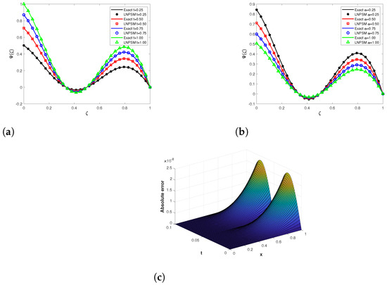
Figure 2.
Comparison between exact and numerical solutions for different values of time and fractional derivatives on for Example 1, where , , and . (a) Effect of time on , where . (b) Effect of on , where . (c) Absolute error between exact solution and LNPSM.
Figure 2b examines the impact of the fractional derivative on at . It demonstrates a decrease in for with increasing , Conversely, the trend reverses for . Figure 2c shows an absolute error comparison between the exact solution and the LNPSM. Table 1 presents a comparative analysis using error norms between our LNPSM and the cubic B-spline collocation method [25] for Example 1. Table 2 shows the experimental order convergent for Example 1 to present the order of the convergent effectively. The error norms provide quantitative insights into the method’s accuracy and effectiveness, showcasing its superiority in approximating the exact solution. These results collectively validate the robustness and applicability of the LNPSM in solving the nonlinear TFBH equation, offering significant advancements over existing numerical techniques.

Table 1.
Comparison of error norms: Conformable LNPSM with cubic B-spline collocation method for Example 1, where , , , and .
Table 2.
Experimental order of convergence for Example 1.
Example 2.
Considering the inhomogeneous TFBH equation,
Considering the following initial and boundary conditions,
with the source term
The exact solution is .
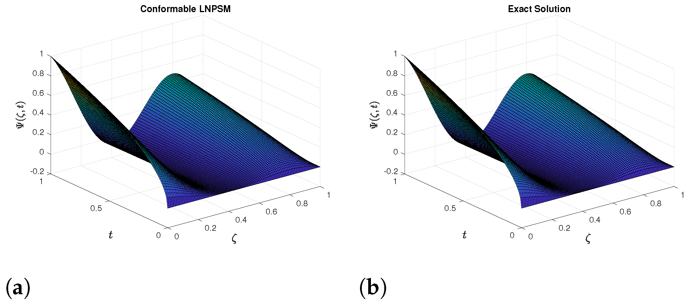
Figure 3a,b display the conformable LNPSM and exact solution 3D mesh plots for Example 2, where , , , and . The figures clearly illustrate that the numerical scheme closely matches the exact solution, demonstrating high accuracy across both spatial and temporal intervals. Figure 4a illustrates the effect of time t on for with . It is evident that increases uniformly as time progresses, reflecting the expected behavior over the specified time interval. Figure 4b examines the impact of the fractional derivative on at . The plot shows that decreases with an increasing , consistent with the anticipated impact of fractional derivatives on the solution profile. Figure 4c shows an absolute error comparison between the exact solution and the LNPSM. Table 3 presents a comparative analysis using error norms between our LNPSM and the cubic B-spline collocation method [25] for Example 2. The error norms serve as a quantitative measure of the method’s accuracy and effectiveness, highlighting its superior performance in approximating the exact solution compared to existing numerical approaches. Table 4 shows the experimental order convergent for Example 2 to present the order of the convergent effectively. These findings underscore the robustness and applicability of the LNPSM in solving nonlinear TFBH equations, demonstrating its potential to advance numerical solutions in fractional differential equations.
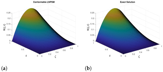
Figure 3.
The 3D Solution profiles for Example 2, where , , and . (a) The conformable NPS solution. (b) The exact Solution.
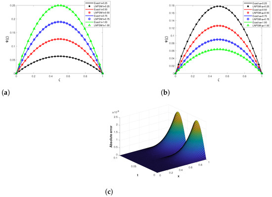
Figure 4.
Comparison between the exact and numerical solutions in different values of time and fractional derivatives on for Example 2, where , and . (a) The effect of time on , where . (b) The effect of on , where . (c) The absolute error between the exact solution and the LNPSM.
Table 3.
Comparison of error norms: LNPSM with cubic B-spline collocation method for Example 2, where , , and .
Table 4.
Experimental order of convergence for Example 2.
7. Conclusions
In conclusion, the logarithmic non-polynomial spline method presented in this study effectively combines conformable derivative, finite difference, and non-polynomial spline techniques to solve the nonlinear inhomogeneous time-fractional Burgers–Huxley equation. The numerical scheme developed demonstrates impressive sixth-order convergence and conditional stability, which are essential for accurate and reliable computations. The method’s accuracy is validated through 3D mesh plots, highlighting its capability to handle complex dynamics influenced by both time and fractional-order variations, as depicted in 2D plots. Comparative analysis with the cubic B-spline collocation method underscores the advantages of our approach in terms of computational efficiency and solution accuracy. Two illustrative examples further confirm the method’s applicability, with and norms providing quantitative evidence of its suitability and effectiveness in practical scenarios of fractional differential equations.
The proposed numerical scheme based on the logarithmic non-polynomial spline method offers several key advantages:
- High Accuracy: The scheme achieves a truncation error with sixth-order convergence, ensuring high precision in numerical solutions.
- Unconditional Stability: The logarithmic non-polynomial spline method is proven to be unconditionally stable, making it reliable for a wide range of problems.
- Superior Performance: Comparative analysis using and norms demonstrates that the method outperforms both the cubic B-spline and Caputo non-polynomial methods.
- Applicability: The method is well-suited for solving conformable time-fractional equations, showing its versatility and effectiveness in complex scenarios.
Author Contributions
Conceptualization, M.A.Y.; data curation, A.A.L.; investigation, M.A.Y., P.O.M. and N.C.; methodology, A.A.L. and R.J.; project administration, P.O.M.; resources, P.O.M.; software, R.P.A.; supervision, A.A.L.; validation, N.C.; visualization, R.P.A.; writing—original draft, M.A.Y. and R.P.A.; writing—review and editing, R.J. and N.C. All authors have read and agreed to the published version of the manuscript.
Funding
The publication of this research was supported by the University of Oradea, Romania.
Institutional Review Board Statement
Not applicable.
Informed Consent Statement
Not applicable.
Data Availability Statement
Data are contained within the article.
Acknowledgments
Researchers Supporting Project number (RSP2024R153), King Saud University, Riyadh, Saudi Arabia.
Conflicts of Interest
The authors declare no conflicts of interest.
Abbreviations
| FDEs | Fractional Differential Equations |
| TFBH | Time-Fractional Burgers–Huxley |
| LNPSM | Logarithmic Non-Polynomial Spline Method |
| KdV | Korteweg–De Vries |
References
- Debnath, L. A brief historical introduction to fractional calculus. Int. J. Math. Educ. Sci. Technol. 2004, 35, 487–501. [Google Scholar] [CrossRef]
- Sivalingam, S.M.; Kumar, P.; Govindaraj, V. A Chebyshev neural network-based numerical scheme to solve distributed-order fractional differential equations. Comput. Math. Appl. 2024, 164, 150–165. [Google Scholar] [CrossRef]
- Abu Arqub, O. Numerical solutions for the Robin time-fractional partial differential equations of heat and fluid flows based on the reproducing kernel algorithm. Int. J. Numer. Methods Heat Fluid Flow 2018, 28, 828–856. [Google Scholar] [CrossRef]
- Bagley, R.L.; Torvik, P.J. A Theoretical Basis for the Application of Fractional Calculus to Viscoelasticity. J. Rheol. 1983, 27, 201–210. [Google Scholar] [CrossRef]
- Uchaikin, V. Fractional Derivatives for Physicists and Engineers; Springer: Berlin/Heidelberg, Germany, 2013. [Google Scholar]
- Mohammed, P.O.; Srivastava, H.M.; Baleanu, D.; Al-Sarairah, E.; Yousif, M.A.; Chorfi, N. Analytical and approximate monotone solutions of the mixed order fractional nabla operators subject to bounded conditions. J. Comput. Appl. Math. 2024, 264, 626–639. [Google Scholar] [CrossRef]
- Yousif, M.A.; Hamasalh, F.K.; Zeeshan, A.; Abdelwahed, M. Efficient simulation of Time-Fractional Korteweg-de Vries equation via conformable-Caputo non-Polynomial spline method. PLoS ONE 2024, 19, e0303760. [Google Scholar] [CrossRef] [PubMed]
- Agarwal, P.; Baleanu, D.; Chen, Y.; Momani, S.; Machado, T. Fractional Calculus; Springer: Berlin/Heidelberg, Germany, 2018. [Google Scholar]
- Podlubny, I. Fractional Differential Equations: An Introduction to Fractional Derivatives, Fractional Differential Equations, to Methods of Their Solution and Some of Their Applications; Academic Press: Cambridge, MA, USA, 1999. [Google Scholar]
- Kilbas, A.A.; Srivastava, H.M.; Trujillo, J.J. Heory and Applications of Fractional Differential Equations; Elsevier: Amsterdam, The Netherlands, 2006. [Google Scholar]
- Sivalingam, S.M.; Govindaraj, V. Physics-informed neural network-based scheme and its error analysis for ψ-Caputo type fractional differential equations. Phys. Scr. 2024, 99, 096002. [Google Scholar] [CrossRef]
- Khalil, R.; Al Horani, M.; Yousef, A.; Sababheh, M. A new definition of fractional derivative. J. Comput. Appl. Math. 2014, 264, 65–70. [Google Scholar] [CrossRef]
- Noureen, R.; Naeem, M.N.; Baleanu, D.; Mohammed, P.O.; Almusawa, M.Y. Application of trigonometric B-spline functions for solving Caputo time fractional gas dynamics equation. AIMS Math. 2023, 8, 25343–25370. [Google Scholar] [CrossRef]
- Sadiya, U.; Inc, M.; Arefin, M.A.; Uddin, M.H. Consistent travelling waves solutions to the non-linear time fractional Klein–Gordon and Sine-Gordon equations through extended tanh-function approach. J. Taibah Univ. Sci. 2022, 16, 594–607. [Google Scholar] [CrossRef]
- Li, M.; Ding, X.; Xu, Q. Non-polynomial spline method for the time-fractional nonlinear Schrödinger equation. Adv. Differ. Equ. 2018, 2018, 318. [Google Scholar] [CrossRef]
- Yousif, M.A.; Hamasalh, F.K. The fractional non-polynomial spline method: Precision and modeling improvements. Math. Comput. Simul. 2024, 218, 512–525. [Google Scholar] [CrossRef]
- Srivastava, H.M.; Saad, K.M.; Hamanah, W.M. Certain new models of the multi-space fractal-fractional Kuramoto-Sivashinsky and Korteweg-de Vries equations. Mathematics 2022, 10, 1089. [Google Scholar] [CrossRef]
- Zou, G.-A. Numerical solutions to time-fractional stochastic partial differential equations. Numer. Algorithms 2019, 82, 553–571. [Google Scholar] [CrossRef]
- Mohamed, M.Z.; Hamza, A.E.; Sedeeg, A.K.H. Conformable double Sumudu transformations an efficient approximation solutions to the fractional coupled Burger’s equation. Ain Shams Eng. J. 2023, 14, 101879. [Google Scholar] [CrossRef]
- Yousif, M.A.; Juan, L.G.; Pshtiwan, O.M.; Nejmeddine, C.; Dumitru, B. A computational study of time-fractional gas dynamics models by means of conformable finite difference method. AIMS Math. 2024, 9, 19843–19858. [Google Scholar] [CrossRef]
- Yousif, M.A.; Hamasalh, F.K. A Hybrid Non-Polynomial Spline Method and Conformable Fractional Continuity Equation. Mathematics 2023, 11, 3799. [Google Scholar] [CrossRef]
- Wang, X.Y.; Zhu, Z.S.; Lu, Y.K. Solitary wave solutions of the generalized Burgers–Huxley equation. J. Phys. A Math. Gen. 1990, 23, 271–274. [Google Scholar] [CrossRef]
- Hodgkin, A.L.; Huxley, A.F. A quantitative description of membrane current and its application to conduction and excitation in nerve. J. Physiol. 1952, 117, 500–544. [Google Scholar] [CrossRef]
- Fitzhugh, R. Mathematical models of excitation and propagation in nerve. In Biological Engineering; Schwan, H.P., Ed.; McGraw-Hill: New York, NY, USA, 1969. [Google Scholar]
- Abdul, M.; Mohsin, K.; Noreen, A.; Dumitru, B. Numerical approximation of inhomogeneous time fractional Burgers–Huxley equation with B-spline functions and Caputo derivative. Eng. Comput. 2022, 38, 885–900. [Google Scholar]
- Deng, X. Traveling wave solutions for the generalized Burgers–Huxley equation. Appl. Math. Comput. 2008, 204, 733–737. [Google Scholar]
- Zhou, S.; Cheng, X. A linearly semi-implicit compact scheme for the Burgers–Huxley equation. Int. J. Comput. Math. 2011, 88, 795–804. [Google Scholar] [CrossRef]
- Gupta, V.; Kadalbajoo, M.K. A singular perturbation approach to solve Burgers–Huxley equation via monotone finite difference scheme on layer adaptive mesh. Commun. Nonlinear Sci. Numer. Simul. 2011, 16, 1825–1844. [Google Scholar] [CrossRef]
- Dehghan, M.; Saray, B.N.; Lakestani, M. Three methods based on the interpolation scaling functions and the mixed collocation finite difference schemes for the numerical solution of the nonlinear generalized Burgers–Huxley equation. Math. Comput. Model 2012, 55, 1129–1142. [Google Scholar] [CrossRef]
- Mohanty, R.K.; Dai, W.; Liu, D. Operator compact method of accuracy two in time and four in space for the solution of time dependent Burgers-Huxley equation. Numer. Algorithms 2015, 70, 591–605. [Google Scholar] [CrossRef]
- Zibaei, S.; Zeinadini, M.; Namjoo, M. Numerical solutions of Burgers–Huxley equation by exact finite difference and NSFD schemes. J. Differ. Equ. Appl. 2016, 22, 1098–1113. [Google Scholar] [CrossRef]
- Yusuf, A.; Aliyu, A.I.; Baleanu, D. Lie symmetry analysis and explicit solutions for the time fractional generalized Burgers–Huxley equation. Opt. Quantum Electron 2018, 50, 94. [Google Scholar]
- Alinia, N.; Zarebnia, M. A numerical algorithm based on a new kind of tension B-spline function for solving Burgers–Huxley equation. Numer. Algorithms 2019, 82, 1121–1142. [Google Scholar] [CrossRef]


Disclaimer/Publisher’s Note: The statements, opinions and data contained in all publications are solely those of the individual author(s) and contributor(s) and not of MDPI and/or the editor(s). MDPI and/or the editor(s) disclaim responsibility for any injury to people or property resulting from any ideas, methods, instructions or products referred to in the content. |
© 2024 by the authors. Licensee MDPI, Basel, Switzerland. This article is an open access article distributed under the terms and conditions of the Creative Commons Attribution (CC BY) license (https://creativecommons.org/licenses/by/4.0/).