Extreme Behavior of Competing Risks with Random Sample Size

Abstract

The advances in science and technology have led to vast amounts of complex and heterogeneous data from multiple sources of random sample length. This paper aims to investigate the extreme behavior of competing risks with random sample sizes. Two accelerated mixed types of stable distributions are obtained as the extreme limit laws of random sampling competing risks under linear and power normalizations, respectively. The theoretical findings are well illustrated by typical examples and numerical studies. The developed methodology and models provide new insights into modeling complex data across numerous fields.

1. Introduction

Extreme value theory (EVT) focuses on modeling extreme events within a sequence of a large number of independent and identically distributed (i.i.d.) random variables. Its applications span diverse fields such as finance, insurance, environmental science, and engineering [1,2]. Let $X_1,X_2,\dots ,X_n$ be a sequence of i.i.d. random variables with a common distribution function (d.f.), F, and denote by $M_n=max(X_1,X_2,\dots ,X_n)$ the sample maxima. The risk $X\sim F$ is called the max-domain attraction of G (cf. Definition 3.3.1 in [2]), if there exist some normalization constants $a_n>0,b_n\in \mathbb{R}$, and a non-degenerate d.f., G, such that (with $\stackrel{d}{\to }$ convergence in distribution or convergence weakly)

$$\mathbb{P}\left(a_n\left(M_n-b_n\right)\le x\right)\stackrel{d}{\to }G\left(x\right)asn\to \infty .$$

(1)

The limit distribution, G, is the so-called generalized extreme value distribution (GEV), satisfying the stability relation $G^n(a_{n}x+b_n)=G\left(x\right),x\in \mathbb{R},n\ge 1$, for every integer n, where $a_n>0$ and $b_n\in \mathbb{R}$ are some suitable constants. The GEV distribution, G, is thus of the l-max stable laws, written as

$$G(x;\gamma ,\mu ,\sigma )=exp\left(-{\left(1+\gamma {\displaystyle \frac{x-\mu }{\sigma }}\right)}_{+}^{-1/\gamma }\right),$$

(2)

where ${\left(x\right)}_{+}=max(x,0)$, the positive part of $x\in \mathbb{R}$. We denote this by $F\in D_l\left(G\right)$. Here, the three parameters $\gamma ,\mu \in \mathbb{R},\sigma >0$ are called the shape, location, and scale parameters. In addition, the tail behavior of the potential risk, X, is well classified into Fréchet, Gumbel, and Weibull domains, corresponding to the cases with $\gamma >,=,<0$, respectively [3].

Given the wide applications of EVT, numerous studies have extensively explored the limit theory similar to Equation (1). Pantcheva [4] extended first the GEV distributions under linear normalization in Equation (1) to the power limit laws $D_p\left(H\right)$, i.e., $X\sim F\in D_p\left(H\right)$ if there exist some power normalization constants ${\alpha }_n,{\beta }_n>0$, and a non-degenerate d.f., H, such that

$$\mathbb{P}\left\{{\alpha }_n{\left|M_n\right|}^{{\beta }_n}\mathrm{sign}\left(M_n\right)\le x\right\}\stackrel{d}{\to }H\left(x\right)$$

(3)

with the sign function $\mathrm{sign}\left(x\right)$ equal 1, $-1$, and 0 for x being positive, negative, and zero, respectively. It is well known that H in Equation (3) is a p-max stable distribution (that is, for any integer $n\ge 1$, there exist suitable constants ${\alpha }_n,{\beta }_n>0$, such that $H^n({\alpha }_n{\left|x\right|}^{{\beta }_n}\mathrm{sign}\left(x\right))=H\left(x\right)$). The limit distribution, H, consists of six types of distributions, which can be written uniformly in the form of Equation (4) below [5]: for some constants $\mu ,\sigma >0$, and $\gamma \in \mathbb{R}$ (recall G is the GEV defined in Equation (2)),

$$\begin{array}{c}\hfill H(x;\gamma ,\mu ,\sigma )=\left\{\begin{array}{cc}G(\log x;\gamma ,\mu ,\sigma ),\hfill & \mathrm{if} \mathrm{the} \mathrm{support} \mathrm{is} \mathrm{included} \mathrm{in} (0,\infty ),\hfill \\ G(-\log (-x);\gamma ,-\mu ,\sigma ),\hfill & \mathrm{otherwise}.\hfill \end{array}\right.\end{array}$$

(4)

In what follows, we denote this by $F\in D_p\left(H\right)$. We refer to [6] for exponential normalization with generalized Pareto families of asymmetric distributions as its limit laws, extending further the p-stable laws under power normalization.

Recently, Cao and Zhang [7] and Hu et al. [8] explored the limit behavior of extremes under linear and power normalization in the scenario of competing risks, with the practical consideration of aggregating multiple heterogeneous information in terms of geography, environment, and socioeconomics [9]. Namely, the studied sample maxima, $M_n$, is actually obtained from k heterogeneous subsamples $X_{j,i},i=1,\dots ,n_j$ from source/population $X_j\sim F_j,j=1,\dots ,k$. This considerate modeling in the big data era is desirable due to the complexity of real applications [10,11]. The limit behavior of $M_n$ obtained for multiple sources is the so-called limit theory of competing risks since

$$\begin{array}{c}\hfill M_n=\underset{1\le j\le k}{max}{M}_{j,n_j}\mathrm{with} M_{j,n_j}=\underset{1\le i\le n_j}{max}{X}_{j,i}.\end{array}$$

(5)

Clearly, the limit laws obtained for competing risks specified in Equation (5), which extend the classical extreme value theory presented in Equations (1) and (3), correspond to the so-called accelerated l-max stable and accelerated p-max stable distributions (see Cao and Zhang [7] (Theorem 2.1) and Hu et al. [8] (Theorem 2.1)). Note that the key condition in determining accelerated limit theory is the interplay of the sample length and the tail behavior among the multiple competing risks.

As the advances of science and technology have led to vast amounts of complex and heterogeneous data from multiple sources of random sample length, a natural question is how the extreme law of competing risks varies in the uncertainty of the sample size involved. This is very common in environmental and financial fields; for instance, the potential extreme claim size among k insured policyholders, each holding the insurance for a $n_j$-day period with heterogeneous claim risk and a total of ${\nu }_{n_j}$ claims [12]. Another example is the extreme daily precipitation among k regions, where each region is exposed to a ${\nu }_{n_j}$-day wet period with different extreme precipitation risks [13]. Although the study of such heterogeneous risks under a random sampling scenario is key in risk management for relevant decision-makers, its extreme behavior remains a significant and unresolved issue. This paper aims to establish the limit theory of competing risks under both linear and power normalization when the sample sizes are random rather than determinant.

Many authors have refined the extreme limit theory of sample maxima from a single risk, X, under linear/power normalization with random sample sizes, ${\nu }_n$, for two common cases:

• Case (I) with a random sample size independent of the basic risk. The random sample $X_1,\dots ,X_n\sim X$ is supposed to be independent of the sample size index ${\nu }_n$. Assume that ${\nu }_n/n$ converges weakly to a non-degenerate distribution function [14,15,16,17];
• Case (II) with a random sample size not independent of the basic risk. There exists a positive-valued variable, V, such that ${\nu }_n/n$ converges to V in probability, allowing the interrelation of the basic risk and sample size index ${\nu }_n$ [14,18,19].

The limit behaviors of extreme samples with random sample sizes were well investigated for a range of extensions, including sample minima [20], extreme order statistics under power normalization [19,21], stationary Gaussian processes [17], stationary chi-processes [16], and recent contributions on multivariate extreme behavior [22].

This paper will focus on the limit behavior of competing extremes (maxima of maxima defined by Equation (5) and minima of minima in Equation (14)) under linear and power normalization, extending the accelerated l-max and p-max stable distributions to be in the mixed form, as we consider that the sample size sequence $\{{\nu }_n,n\ge 1\}$ is a random sequence satisfying conditions indicated in Cases I and II above. The theoretical results will be illustrated by typical examples with random sample sizes, ${\nu }_n$, following time-shifted Poisson, (negative) binomial distributions, and numerical studies (cf. Section 3). Our theoretical findings are expected to be applied in finance, insurance, and hydrology [23,24]. The developed methodology and models provide new insights into modeling complex data across numerous fields.

The remainder of the paper is organized as follows. Section 2 presents the main results for maxima of maxima under both linear and power normalization with sample sizes. Extensional results for competing minima and typical examples are given in Section 3. Numerical studies illustrating our theoretical findings are presented in Section 4. The proofs of all theoretical results are deferred to Appendix A.

2. Main Results

Notation. Recall that the competing risks defined in Equation (5) are generated from k independent samples of size $n_j$’s from risks $X_j\sim F_j,1\le j\le k$. Let $\{{\nu }_{n_j},n_j\ge 1\},$ a random sequence from ${\nu }_j,1\le j\le k$, which are mutually independent, positive integer-valued variables, stand for the random sample size. Similar to Equation (5), we write

$$M_{{\nu }_n}=\underset{1\le j\le k}{max}{M}_{j,{\nu }_{n_j}}\mathrm{with}{M}_{j,{\nu }_{n_j}}=\underset{1\le i\le {\nu }_{n_j}}{max}{X}_{j,i}.$$

(6)

Here, ${\nu }_n:={\sum }_{1\le j\le k}{\nu }_{n_j}$ and $n={\sum }_{j=1}^k{n}_j$. Throughout this paper, for any risk, X, following a cumulative distribution function (cdf), F, we write $\underline{F}\left(x\right):=1-{lim}_{t\uparrow -x}F\left(t\right)$, standing for the cdf of $-X$. Further, we denote by $\stackrel{p}{\to }$ the convergence in probability, and all limits are taken as ${min}_{1\le j\le k}{n}_j\to \infty$.

To simplify the notation, in what follows, we consider competing risks from two sources, namely $k=2$. We will present the limit behavior of $M_{{\nu }_n}$ for Cases I and II in Section 2.1 and Section 2.2, respectively.

2.1. Limit Theorem for Case (I) with Independent Sample Size

In this section, we present our main results concerning the limit behavior of competing risks under linear and power normalization, as detailed in Theorems 1 and 2, respectively. We focus on the following random sample size scenario: assume that there exist k positive variables $V_j,1\le j\le k$, such that

$${\displaystyle \frac{{\nu }_{n_j}}{n_j}}\stackrel{d}{\to }{V}_j.$$

(7)

Condition (7) is commonly used for the limit behavior of extremes with random sample sizes [16,21,25]. In general, one may consider a random stopping sampling process [26]. Typical examples of random sample sizes satisfying Equation (7) are given in Section 3.2 (cf. Examples 1∼3); see also Peng et al. [15] for more examples. In addition, it is worthy to note that, under condition (7), the $V_j$’s inherit the mutual independence of the random sample size sequences $\{{\nu }_{n_j},n_j\ge 1\},j=1,2,\dots ,k$.

1. Limit behavior of $M_{{\nu }_n}$ under linear normalization. Clearly, for $F_j\in D_l\left(G_j\right)$, there exist some constants $a_{j,n_j}>0,b_{j,n_j}\in \mathbb{R}$, such that $M_{j,n_j}$ satisfies Equation (1) as $n_j\to \infty$. It follows further by Theorem 6.2.1 in Galambos [18] (Ch.6, p.330) that, under condition (7), we can find a subsequence ${\nu }_{n_j^{\prime }}/n_j^{\prime }\stackrel{p}{\to }{V}_j$ by Skorokhod representation theorem and $a_{j,n_j^{\prime }}(M_{j,{\nu }_{n_j^{\prime }}}-b_{j,n_j^{\prime }})\stackrel{d}{\to }{L}_j$, a mixed GEV distribution defined by

$$L_j\left(x\right)={\int }_0^{\infty }{G}_j^z\left(x\right)d\mathbb{P}\left\{V_j\le z\right\}.$$

(8)

Below, we will show in Theorem 1 that, under condition (7), the limit theorem for competing extremes, $M_{{\nu }_n}$, holds with an accelerated mixed GEV distribution, which can be written as a product of independent $L_j$’s.

Theorem 1.

Let $M_{{\nu }_n}$ be given by Equation (6) with the basic risks $X_j\sim F_j,j=1,2$, and random sample sizes ${\nu }_1,{\nu }_2$ mutually independent. Assume conditions (1) and (7) hold for sample maxima $M_{j,n_j}$ with suitable constants $a_{j,n_j},b_{j,n_j}$, and the random sample size ${\nu }_{n_j}\sim {\nu }_j,j=1,2$. Suppose further that there exist two constants $a\in [0,\infty ]$ and $b\in \mathbb{R}$, such that

$$a_n:={\displaystyle \frac{a_{1,n_1}}{a_{2,n_2}}}\to a,b_n:=a_{1,n_1}(b_{2,n_2}-b_{1,n_1})\to b$$

(9)

 as $min(n_1,n_2)\to \infty$.

(i). 

If Equation (9) holds with $a>0$ and $b<\infty$, then

$$\mathbb{P}\left(a_{2,n_2}(M_{{\nu }_n}-b_{2,n_2})\le x\right)\stackrel{d}{\to }{L}_1\left(ax+b\right)L_2\left(x\right).$$

(ii). 

If Equation (9) holds with $a=0$ and $b=\infty$, then

$$\mathbb{P}\left(a_{2,n_2}(M_{{\nu }_n}-b_{2,n_2})\le x\right)\stackrel{d}{\to }{L}_2\left(x\right).$$

Here, $L_j,j=1,2$ are given by Equation (8).

Remark 1. (a) Theorem 1 is reduced to Theorem 2.1 by Cao and Zhang [7] if all $V_j$’s are degenerate at one (that is, ${\nu }_{n_j}\equiv n_j$ in probability), the limit theorem for competing maxima with determinant sample size.

(b) In addition, the two results in (i) and (ii) correspond to the cases for two competing risks being comparable tails with a balanced sampling process and the dominated case, respectively.

(c) In general, our results introduce a fairly larger class of accelerated mixed GEV distribution, as a product of the mixed GEV distributions written in the form of Equation (8).

2. Limit behavior of $M_{{\nu }_n}$ under power normalization. Clearly, for $F_j\in D_p\left(H_j\right)$, there exist ${\alpha }_{j,n_j},{\beta }_{j,n_j}>0$, such that $M_{j,n_j}$ satisfies Equation (3) as $n_j\to \infty$. We will show in Theorem 2 that, under condition (7), the limit theorem for competing extremes, $M_{{\nu }_n}$, holds with an accelerated mixed distribution, P, which can be written as the product of $P_j$’s given below

$$P_j\left(x\right)={\int }_0^{\infty }{\left(H_j\left(x\right)\right)}^{z}d\mathbb{P}\left\{V_j\le z\right\}.$$

(10)

Here, $H_j,j=1,2$ are of the same p-type of H defined in Equation (4).

Theorem 2.

Let $M_{{\nu }_n}$ be given by Equation (6) with the basic risks $X_j\sim F_j,j=1,2$, and random sample sizes ${\nu }_1,{\nu }_2$ mutually independent. Assume conditions (3) and (7) hold for sample maxima $M_{j,n_j}$ with suitable constants ${\alpha }_{j,n_j},{\beta }_{j,n_j}>0$, and the random sample size ${\nu }_{n_j}\sim {\nu }_j,j=1,2$. Suppose further there exist two non-negative constants α and β such that

$${\alpha }_n:={\alpha }_{1,n_1}{\left({\displaystyle \frac{1}{{\alpha }_{2,n_2}}}\right)}^{{\displaystyle \frac{{\beta }_{1,n_1}}{{\beta }_{2,n_2}}}}\to \alpha ,{\beta }_n:={\displaystyle \frac{{\beta }_{1,n_1}}{{\beta }_{2,n_2}}}\to \beta$$

(11)

as $min(n_1,n_2)\to \infty$. The following claims hold with mixed p-stable distributions $P_j,j=1,2$ defined by Equation (10).

(i). 

If condition (11) holds with two positive constants α and β, then

$$\begin{array}{c}\hfill \mathbb{P}\left\{{\alpha }_{2,n_2}{\left|M_{{\nu }_n}\right|}^{{\beta }_{2,n_2}}\mathrm{sign}\left(M_{{\nu }_n}\right)\le x\right\}\stackrel{d}{\to }{P}_1\left({\alpha \left|x\right|}^{\beta }\mathrm{sign}\left(x\right)\right)P_2\left(x\right).\end{array}$$

(12)

(ii). 

The following limit distribution holds

$$\mathbb{P}\left\{{\alpha }_{2,n_2}{\left|M_{{\nu }_n}\right|}^{{\beta }_{2,n_2}}\mathrm{sign}\left(M_{{\nu }_n}\right)\le x\right\}\stackrel{d}{\to }{P}_2\left(x\right)$$

provided that one of the following four conditions is satisfied (notation: $x_1^{*}:=inf\{x:H_1\left(x\right)<1\}$, the right endpoint of $H_1$)

(a). 

When $H_2$ is one of the same p-types of $G(\log x;\gamma ,\mu ,\sigma )$, and $H_1$ is one of the same p-types of $G(-\log (-x);\gamma ,-\mu ,\sigma )$.

(b). 

When $H_2$ is one of the same p-types of $G(\log x;\gamma ,\mu ,\sigma )$, and $H_1$ is one of the same p-types of $G(\log x;\gamma ,\mu ,\sigma )$ for $\gamma \ge 0$. In addition, Equation (11) holds with $\alpha =\infty$ and $0\le \beta <\infty$.

(c). 

When $H_2$ is one of the same p-types of $G(\log x;\gamma ,\mu ,\sigma )$, and $H_1$ is one of the same p-types of $G(\log x;\gamma ,\mu ,\sigma )$ for $\gamma <0$. In addition, Equation (11) holds with $x_1^{*}\le \alpha <\infty$ and $\beta =0$ or $\alpha =\infty$ and $0\le \beta <\infty$.

(d). 

When both $H_1$ and $H_2$ are one of the same p-types of $G(-\log (-x);\gamma ,-\mu ,\sigma )$. In addition, Equation (11) holds with $0\le \alpha \le -x_1^{*}$ and $\beta =0$ or $\alpha =0$ and $0\le \beta <\infty$.

Remark 2.  (a) Theorem 2 is reduced to the extreme limit behavior of competing risks with determinant sample size if all $V_j$’s are degenerate at one, which was extensively discussed in Hu et al. [8]. The random sampling size scenarios are very common in practice. For instance, in physics and insurance fields, ${\nu }_n$ follows a shifted Poisson df with mean ${\lambda }_n$ such that ${\lambda }_n\sim n$. For more examples, see Example 1 below and Remark 2.2 by Abd Elgawad et al. [27].

(b) In addition, the two results in i) and ii) correspond to the two different cases with $\alpha \beta >0$ and $\alpha \beta =0,\infty$ in condition (11). These results illustrate the limit behavior of two competing risks with comparable tails and a balanced sampling process and the dominated case, respectively.

(c) Theorem 2 extends Theorem 2.1 by Barakat and Nigm [19] for a non-competing risk scenario, where the extremes are from one single source. In general, the accelerated mixed power-stable distributions family is a larger class including those of form in Equation (10).

2.2. Limit Theorem for Case (II) with Non-Independent Sample Size

In this section, we focus on Case (II), where we relax the independent condition between the basic risk and random sample size. On the other hand, we need to strengthen the convergence in distribution as the convergence in probability, as stated below. Assume that there exist positive random variables $V_j,j=1,2$, such that

$${\nu }_{n_j}/n_j\stackrel{p}{\to }{V}_j,j=1,2.$$

(13)

Theorem 3.

Let $M_{{\nu }_n}$ be given by Equation (6) with two random sampling maxima from two independent pairs of basic risk and sample size $(X_j,{\nu }_j),j=1,2$. Suppose that conditions (9) and (13) hold for $X_j\sim F_j\in D_l\left(G_j\right)$ with Equation (2) satisfied for $M_{j,n_j}$ and $a_{j,n_j},b_{j,n_j},j=1,2$. Then the claim in Theorem 1 holds.

Theorem 4.

Let $M_{{\nu }_n}$ be given by Equation (6) with two random sampling maxima from two independent pairs of basic risk and sample size $(X_j,{\nu }_j),j=1,2$. Suppose that conditions (11) and (13) hold for $X_j\sim F_j\in D_p\left(H_j\right)$ with Equation (2) satisfied for $M_{j,n_j}$ and ${\alpha }_{j,n_j},{\beta }_{j,n_j},j=1,2$. Then the claim in Theorem 2 holds.

Remark 3.

Recalling that G and H given by Equations (2) and (4) are the so-called l-max stable and p-max stable distributions, we call L and P the accelerated mixed l-max stable and the accelerated mixed p-max stable distributions if they can be written as a product of $L_j$ and $P_j$, respectively. Thus, the limit laws obtained by Theorems 3 and 4 correspond to fairly larger families of accelerated mixed l-max stable and accelerated mixed p-max stable distributions, respectively.

3. Extension and Examples

In this section, we first extend our results for competing minima risks in Section 3.1, and then present typical examples of random sizes with specific mixed extreme distributions in Section 3.2.

3.1. Extreme Limit Theory for Competing Minima Risks

In some practical applications, such as the lifetime analysis in reliability studies or race time of athletes in physical studies, extreme minima play an important role. As we will see in Corollaries 1 and 2 below, analytical claims follow for competing risks with random sample sizes in terms of minima of minima. Essentially, noting that the right tail behavior of $X_j\sim F_j$ is demonstrated by its sample maxima, $M_{j,n_j}$, the left tail behavior of $-X_j\sim {\underline{F}}_j\left(x\right)$ can be shown by the sample minima ${\underline{m}}_{j,n_j}=min(-X_{j,1},\dots ,-X_{j,n_j})$. Further, the left tail behavior of $-X$ can be obtained through the study of the right tail of X since (cf. Theorem 1.8.3 in Leadbetter et al. [1] and Grigelionis [28])

$$\begin{array}{c}\hfill {\underline{m}}_n=\underset{1\le j\le k}{min}{\underline{m}}_{j,n_j}=-\underset{1\le j\le k}{max}{M}_{j,n_j}=-M_n.\end{array}$$

(14)

Noting that, the condition that $F_j\in D_l\left(G_j\right)$, i.e., there exist some constants $a_{j,n_j}>0,b_{j,n_j}\in \mathbb{R}$, such that $M_{j,n_j}$ satisfies Equation (1) as $n_j\to \infty$, is equivalent that

$$\mathbb{P}\left(a_{j,n_j}({\underline{m}}_{j,n_j}+b_{j,n_j})\le x\right)\stackrel{d}{\to }{\underline{G}}_j\left(x\right),$$

(15)

where $G_j$ is of the same l-type of GEV distributions given in Equation (2).

Corollary 1.

Suppose the same conditions as for Theorems 1 or 3 are satisfied.

(i). 

If Equation (9) holds with $a>0$ and $b<\infty$, then

$$\mathbb{P}\left(a_{2,n_2}({\underline{m}}_{{\nu }_n}+b_{2,n_2})\le x\right)\stackrel{d}{\to }1-L_1\left(-(ax-b)\right)L_2(-x).$$

(ii). 

If Equation (9) holds with $a=0$ and $b=\infty$, then

$$\mathbb{P}\left(a_{2,n_2}({\underline{m}}_{{\nu }_n}+b_{2,n_2})\le x\right)\stackrel{d}{\to }1-L_2(-x).$$

Here, $L_j,j=1,2$ are given by Equation (8).

Noting that ${\alpha }_n|{\underline{m}}_n{|}^{{\beta }_n}\mathrm{sign}\left({\underline{m}}_n\right)=-{\alpha }_n{\left|M_n\right|}^{{\beta }_n}\mathrm{sign}\left(M_n\right)$, the following corollary holds for the power normalized minima of minima specified in Equation (14).

Corollary 2.

Suppose that the same conditions as for Theorems 2 or 4 are satisfied. The following claims hold for ${\underline{P}}_j\left(x\right),j=1,2$, with $P_j$ the mixed $H_j$ distributions defined in Equation (10).

(i). 

If condition (11) holds with two positive constants α and β, then

$$\begin{array}{c}\hfill \mathbb{P}\left\{{\alpha }_{2,n_2}{\left|{\underline{m}}_{{\nu }_n}\right|}^{{\beta }_{2,n_2}}\mathrm{sign}\left({\underline{m}}_{{\nu }_n}\right)\le x\right\}\stackrel{d}{\to }1-P_1\left(-{\alpha \left|x\right|}^{\beta }\mathrm{sign}\left(x\right)\right)P_2(-x).\end{array}$$

(ii). 

The following limit distribution holds

$$\mathbb{P}\left\{{\alpha }_{2,n_2}{\left|{\underline{m}}_{{\nu }_n}\right|}^{{\beta }_{2,n_2}}\mathrm{sign}\left({\underline{m}}_{{\nu }_n}\right)\le x\right\}\stackrel{d}{\to }1-P_2(-x)$$

provided that one of the conditions (a)∼(d) in Theorem 2 holds.

Remark 4.

Recalling that $\underline{G}$ and $\underline{H}$ are the so-called l-min stable and p-min stable distributions [28] (Corollary 1), if G and H are given by Equations (2) and (4), we call $\underline{L}$ and $\underline{P}$ the mixed l-min stable and the mixed p-min stable distributions if they can be written as a product of ${\underline{L}}_j$ and ${\underline{P}}_j$, respectively.

3.2. Examples

Below, we will give three examples (Examples 1∼3) to illustrate our main results obtained in Theorems 1 and 2. Specifically, we consider that random sample size follows, respectively, time-shifted versions of Poisson or binomial distribution, as well as geometric and negative binomial distributions with relevant parameters satisfying certain average stable conditions [15].

Example 1

(Time-shifted binomial/Poisson distributed random sample size). Let ${\nu }_n$ follow a time-shifted binomial distribution with probability mass function (pmf) given as

$$\mathbb{P}\left\{{\nu }_n=k+m\right\}=\left({\displaystyle \genfrac{}{}{0pt}{}{l_n}{k}}\right)p_n^k{q}_n^{l_n-k},k+m=m,m+1,\dots ,l_n+m.$$

If $l_n{p}_n\to 1$, then ${\nu }_n/n$ converges in probability to one. Similarly, for a time-shifted Poisson distributed ${\nu }_n\stackrel{d}{=}m+Poisson\left({\lambda }_n\right)$ with ${\lambda }_n/n\to 1$, then ${\nu }_n/n$ converges in probability to 1 [15] (Lemmas 4.3). For the random sample size aforementioned, the claims of Theorems 1 and 2 follow as the reduced determinant random size cases, see Remarks 1(a) and 2(a).

Example 2

(Time-shifted geometric distributed sample size). In the case of linear normalization, with G being one of the three l-types of distributions, say $G(x;\gamma ,\mu ,\sigma )$ specified in Equation (2). Suppose that the random sample size, ${\nu }_{n_j}$, follows a geometric distribution with mean $n_j$. We have ${\nu }_{n_j}\approx n_{j}V$ in distribution with a random scale, V, following a standard exponential distribution. Consequently, Theorem 1 holds with an accelerated mixed l-max stable distribution, $LL$, which is the product of mixed l-max stable distributions of form L as described below.

$$\begin{array}{c}{\displaystyle L(x;\gamma ,\mu ,\sigma )={\int }_0^{\infty }{\left(G(x;\gamma ,\mu ,\sigma )\right)}^{z}d(1-{\mathrm{e}}^{-z})}\hfill \\ \hspace{1em}\hspace{1em}={\int }_0^{\infty }exp\left(-z\left({\left(1+\gamma {\displaystyle \frac{x-\mu }{\sigma }}\right)}_{+}^{-1/\gamma }+1\right)\right)dz={\displaystyle \frac{1}{1+{\left(1+\gamma \frac{x-\mu }{\sigma }\right)}_{+}^{-1/\gamma }}},\hfill \end{array}$$

which is taken as its limit $1/[1+exp\left(-(x-\mu )/\sigma \right),x>\mu$ for $\gamma =0$.

Similarly, for the power normalization case, recalling H is specified in Equation (4), as the p-max type of limit distributions, Theorem 2 follows with an accelerated mixed p-max stable distribution, $PP$, the product of mixed p-max stable distribution P, as described below (cf. Barakat and Nigm [19] [Example 2.1]).

$$\begin{array}{c}{\displaystyle P(x;\gamma ,\mu ,\sigma )={\int }_0^{\infty }{\left(H(x;\gamma ,\mu ,\sigma )\right)}^{z}d(1-{\mathrm{e}}^{-z})}\hfill \\ \hspace{1em}\hspace{1em}=\left\{\begin{array}{cc}{\int }_0^{\infty }{G}^z(\log x;\gamma ,\mu ,\sigma ){\mathrm{e}}^{-z}dz,\hfill & \mathit{if} \mathit{the} \mathit{support} \mathit{is} \mathit{included} \mathit{in} (0,\infty ),\hfill \\ {\int }_0^{\infty }{G}^z(-\log (-x);\gamma ,-\mu ,\sigma ){\mathrm{e}}^{-z}dz,\hfill & \mathit{otherwise},\hfill \end{array}\right.\hfill \\ \hspace{1em}\hspace{1em}=\left\{\begin{array}{cc}{\displaystyle \frac{1}{{\displaystyle 1+{\left(1+\gamma \frac{\log x-\mu }{\sigma }\right)}_{+}^{-1/\gamma }}}},\hfill & \mathit{if} \mathit{the} \mathit{support} \mathit{is} \mathit{included} \mathit{in} (0,\infty ),\hfill \\ {\displaystyle \frac{1}{{\displaystyle 1+{\left(1+\gamma \frac{-\log (-x)+\mu }{\sigma }\right)}_{+}^{-1/\gamma }}}},\hfill & \mathit{otherwise}.\hfill \end{array}\right.\hfill \end{array}$$

Example 3

(Time-shifted negative binomial distributed sample size). As an extension of m-shifted geometric distributions, we consider time-shifted negative binomial distributed sample size ${\nu }_n$ with $r\ge 1$ given by

$$\mathbb{P}\left\{{\nu }_n=k\right\}=\left(\begin{array}{c}-r\\ k-rm\end{array}\right)p_n^r{[-(1-p_n)]}^{k-rm},k=rm,rm+1,\dots .$$

It follows from Lemma 4.1 by Peng et al. [15] that, as $n{p}_n\to 1$, we have that ${\nu }_n/n$ converges in distribution to V, a gamma random variable with shape parameter r and scale parameter 1, i.e., the cdf of V is given by

$$F_V\left(z\right)=\mathbb{P}\left\{V\le z\right\}={\int }_0^z{\displaystyle \frac{1}{\Gamma \left(r\right)}}{t}^{r-1}{\mathrm{e}}^{-t}dt,z>0,$$

where $\Gamma (·)$ denotes the gamma function. It follows by Theorem 1 that

$$\begin{array}{c}{\displaystyle L(x;\gamma ,\mu ,\sigma )={\int }_0^{\infty }{\left(G(x;\gamma ,\mu ,\sigma )\right)}^{z}d{F}_V\left(z\right)}\hfill \\ \hspace{1em}\hspace{1em}={\int }_0^{\infty }{\displaystyle \frac{1}{\Gamma \left(r\right)}}{z}^{r-1}exp\left(-z\left({\left(1+\gamma {\displaystyle \frac{x-\mu }{\sigma }}\right)}_{+}^{-1/\gamma }+1\right)\right)dz\hfill \\ \hspace{1em}\hspace{1em}={\left[1+{\left(1+\gamma {\displaystyle \frac{x-\mu }{\sigma }}\right)}_{+}^{-1/\gamma }\right]}^{-r}.\hfill \end{array}$$

Similarly, Theorem 2 follows with the accelerated mixed p-max stable distributions, which are products of cdfs of form P given below.

$$\begin{array}{c}\hfill P(x;\gamma ,\mu ,\sigma )=\left\{\begin{array}{cc}{\left[1+{\left(1+\gamma {\displaystyle \frac{\log x-\mu }{\sigma }}\right)}_{+}^{-1/\gamma }\right]}^{-r},\hfill & \mathit{if} \mathit{the} \mathit{support} \mathit{is} \mathit{included} \mathit{in} (0,\infty ),\hfill \\ {\left[1+{\left(1+\gamma {\displaystyle \frac{-\log (-x)+\mu }{\sigma }}\right)}_{+}^{-1/\gamma }\right]}^{-r},\hfill & \mathit{otherwise}.\hfill \end{array}\right.\end{array}$$

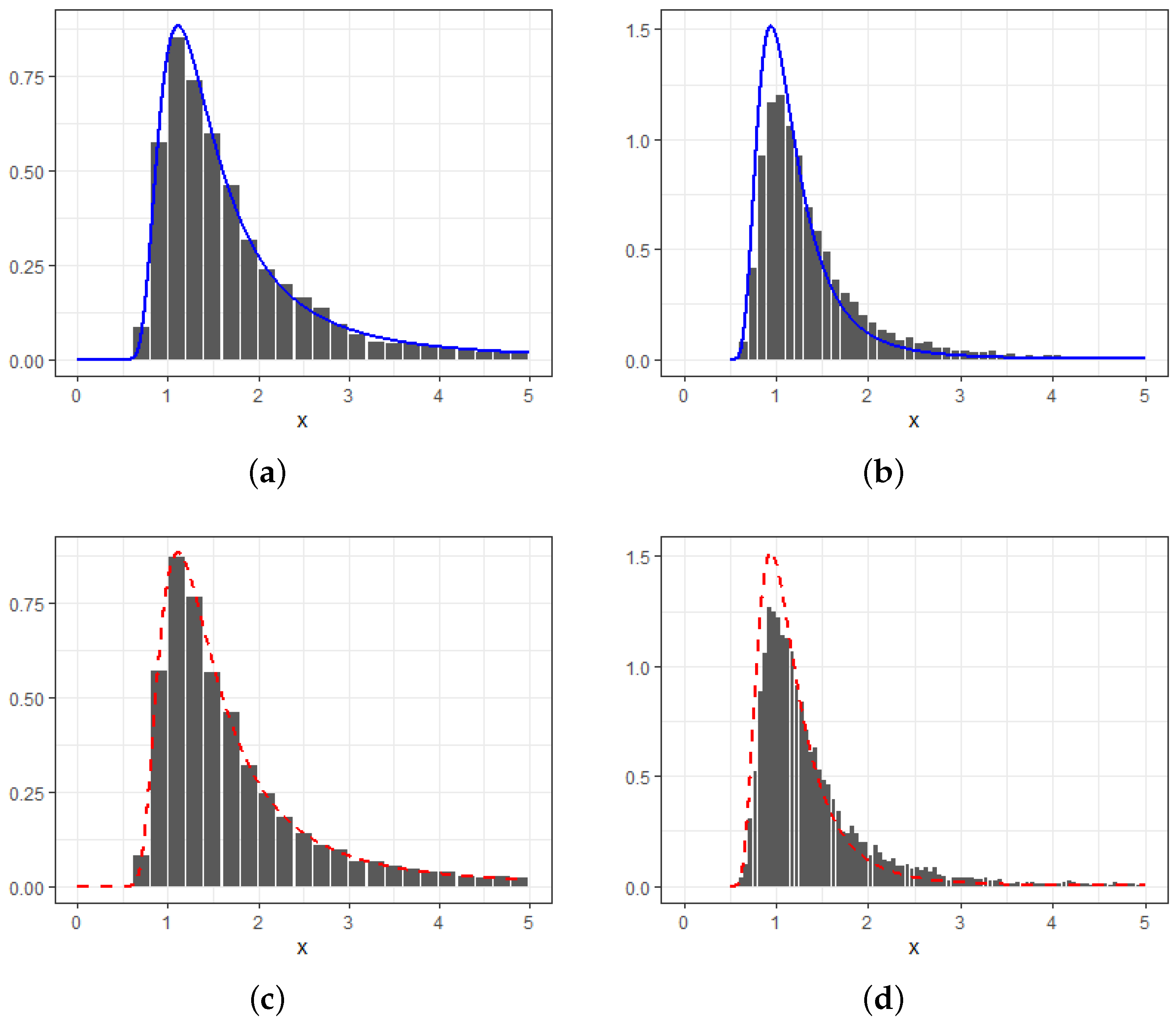
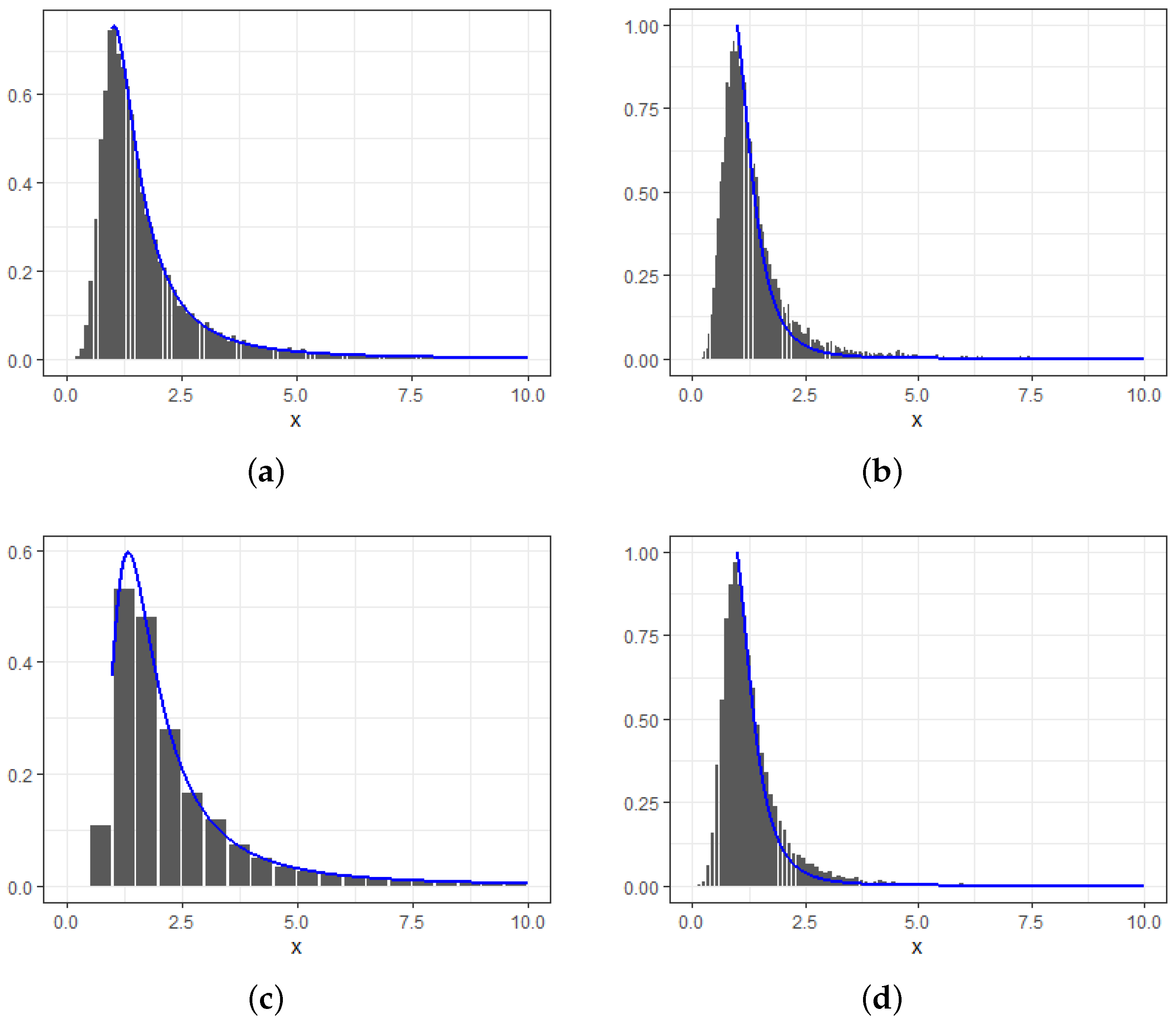
4. Numerical Studies

We will conduct a Monte Carlo simulation to illustrate Theorems 1 and 2 with the m-shifted random sample size given in Examples 1∼2. In the following simulations, we set the shift parameter $m=5$ for all time-shifted random sample size distributions. The basic risks $X_1,X_2$ are drawn from Pareto$\left({\alpha }_1\right)$ and Pareto$\left({\alpha }_2\right)$ (recall the cdf of Pareto$\left(\alpha \right)$ is given as $\mathbb{P}\left\{X\le x\right\}=1-x^{-\alpha },x>1$), and the random sample sizes ${\nu }_{n_1},{\nu }_{n_2}$ are supposed to be mutually independent. Additionally, the repeated time is taken as $R=10,000$. We will illustrate our main results specified in Theorems 1 using the three examples given in Section 3.2 above.

1. Comparison of Pareto competing extremes with determinant sample size and Poisson distributed random sample size. In Figure 1, we will demonstrate that the competing extremes with a Poisson distributed sample size are similar to the case with a non-random sample size. Let ${\nu }_{n_j}$ follow m-shifted Poisson distribution with mean parameters $n_j,j=1,2$. We then generate competing Pareto extremes with basic risks following Pareto$\left({\alpha }_j\right)$ for given ${\alpha }_j>0,j=1,2.$ It follows from Theorems 1, 2 and Example 1 together with Example 4.6 by Hu et al. [8] that (recall $\Phi (x;\alpha )=exp\left(-x^{-\alpha }\right),x>0,\alpha >0$, the Fréchet distribution)

• For $n_2=n_1$ or $n_2=n_1^c$ with $c>{\alpha }_2/{\alpha }_1$, we have

  $$n_2^{-1/{\alpha }_2}{M}_{{\nu }_n}\stackrel{d}{\to }\Phi (x;{\alpha }_2),n_2^{-1}{M}_{{\nu }_n}^{{\alpha }_2}\stackrel{d}{\to }\Phi (x;1).$$
• For $n_2=n_1^c$ with $c={\alpha }_2/{\alpha }_1$, we have

  $$n_2^{-1/{\alpha }_2}{M}_{{\nu }_n}\stackrel{d}{\to }\Phi (x;{\alpha }_1)\Phi (x;{\alpha }_2),n_2^{-1}{M}_{{\nu }_n}^{{\alpha }_2}\stackrel{d}{\to }\Phi (x;{\alpha }_1/{\alpha }_2)\Phi (x;1).$$

Note that the power normalized extremes behave similarly to the linear normalized ones, up to a power transformation. Therefore, we will focus on the behavior of linear normalization in the numerical studies presented below.

In Figure 1, we take ${\alpha }_1=2,{\alpha }_2=4$ and $n_1=100,n_2=n_1^c$ with $c=2,2.5$ to show the above two cases. Overall, the competing Pareto extremes are well fitted by the accelerated GEV distribution for the non-random sample size, with a slightly better fit compared with the random sample size cases. Furthermore, the accelerated GEV approximation (Figure 1a,c) is relatively closer to the empirical competing extremes than the dominated case.

2. Comparison of Pareto competing extremes with geometric distributed and negative binomial distributed sample size. We consider the maxima of maxima $M_{{\nu }_n}$ with basic risks $X_j\sim Pareto\left({\alpha }_j\right)$ and random sample sizes ${\nu }_{n_j}$ following m-shifted negative binomial distribution with probability $1/n_j,j=1,2$, and $r\ge 1$. It follows by Example 4.6 by Hu et al. [8], Theorem 1 (a, b), and Example 3 that, with $\tilde{L}(x;\alpha )={[1+x^{-\alpha }]}^{-r},x>0$

• For $n_2=n_1$ or $n_2=n_1^c$ with $c>{\alpha }_2/{\alpha }_1$, we have $n_2^{-1/{\alpha }_2}{M}_{{\nu }_n}\stackrel{d}{\to }\tilde{L}(x;{\alpha }_2).$
• For $n_2=n_1^c$ with $c={\alpha }_2/{\alpha }_1$, we have $n_2^{-1/{\alpha }_2}{M}_{{\nu }_n}\stackrel{d}{\to }\tilde{L}(x;{\alpha }_1)\tilde{L}(x;{\alpha }_2).$

Thus, its density function is given by

$$\begin{array}{c}\hfill l(x;{\alpha }_1,{\alpha }_2)=\left\{\begin{array}{cc}{\displaystyle \frac{d\tilde{L}(x;{\alpha }_2)}{dx}}={\displaystyle \frac{r{\alpha }_2}{x^{{\alpha }_2+1}{(1+x^{-{\alpha }_2})}^{r+1}}},\hfill & \\ {\displaystyle \frac{d\tilde{L}(x;{\alpha }_1)\tilde{L}(x;{\alpha }_2)}{dx}}={\displaystyle \frac{r{\alpha }_1{x}^{-{\alpha }_1-1}}{{(1+x^{-{\alpha }_1})}^{r+1}{(1+x^{-{\alpha }_2})}^r}}+{\displaystyle \frac{r{\alpha }_2{x}^{-{\alpha }_2-1}}{{(1+x^{-{\alpha }_2})}^{r+1}{(1+x^{-{\alpha }_1})}^r}},\hfill \end{array}\right.\end{array}$$

(16)

In Figure 2, we set $n_1=100,n_2=n_1^c$ with $c=2,2.5$ in (a, c) and (b, d), respectively. The random sample size follows a 5-shifted negative binomial distribution with $r=1$ in (a, b) (namely geometric distribution), $r=2$ in (c, d), and probability $1/n_j,j=1,2$. The Pareto basic risks are set with ${\alpha }_1=2$ and ${\alpha }_2=4$. Consequently, the sub-maxima are completely competing when $n_2=n_1^2$, resulting in the accelerated mixed extreme limit distributions as shown in Figure 2a,c. In contrast, the dominated limit behavior is given in Figure 2b,d as $n_2=n_1^{2.5}$.

In general, our theoretical density curve given by Equation (16) approximates the histogram very well (Figure 2). Further, we see that the approximation with geometric distributed random size is slightly better than the negative binomial case. In addition, the approximation for the dominated case (Figure 2d) is slightly better than the accelerated case when negative binomial random size applies.

References

1. Leadbetter, M.R.; Lindgren, G.; Rootzén, H. Extremes and Related Properties of Random Sequences and Processes; Springer: New York, NY, USA, 1983. [Google Scholar]
2. Embrechts, P.; Kluppelberg, C.; Mikosch, T. Modelling Extremal Events; Stochastic Modelling and Applied Probability; Springer: Berlin/Heidelberg, Germany, 1997. [Google Scholar]
3. Beirlant, J.; Teugels, J.L. Limit distributions for compounded sums of extreme order statistics. J. Appl. Probab. 1992, 29, 557–574. [Google Scholar] [CrossRef]
4. Pantcheva, E. Limit Theorems for Extreme Order Statistics under Nonlinear Normalization; Springer: Berlin/Heidelberg, Germany, 1985; pp. 284–309. [Google Scholar]
5. Nasri-Roudsari, D. Limit distributions of generalized order statistics under power normalization. Commun. Stat.-Theory Methods 1999, 28, 1379–1389. [Google Scholar] [CrossRef]
6. Barakat, H.M.; Khaled, O.M.; Rakha, N.K. Modeling of extreme values via exponential normalization compared with linear and power normalization. Symmetry 2020, 12, 1876. [Google Scholar] [CrossRef]
7. Cao, W.; Zhang, Z. New extreme value theory for maxima of maxima. Stat. Theory Relat. Fields 2021, 5, 232–252. [Google Scholar] [CrossRef]
8. Hu, K.; Wang, K.; Constantinescu, C.; Zhang, Z.; Ling, C. Extreme Limit Theory of Competing Risks under Power Normalization. arXiv 2023, arXiv:2305.02742. [Google Scholar]
9. Chen, Y.; Guo, K.; Ji, Q.; Zhang, D. “Not all climate risks are alike”: Heterogeneous responses of financial firms to natural disasters in China. Financ. Res. Lett. 2023, 52, 103538. [Google Scholar] [CrossRef]
10. Cui, Q.; Xu, Y.; Zhang, Z.; Chan, V. Max-linear regression models with regularization. J. Econom. 2021, 222, 579–600. [Google Scholar] [CrossRef]
11. Zhang, Z. Five critical genes related to seven COVID-19 subtypes: A data science discovery. J. Data Sci. 2021, 19, 142–150. [Google Scholar] [CrossRef]
12. Soliman, A.A. Bayes Prediction in a Pareto Lifetime Model with Random Sample Size. J. R. Stat. Soc. Ser. 2000, 49, 51–62. [Google Scholar] [CrossRef]
13. Korolev, V.; Gorshenin, A. Probability models and statistical tests for extreme precipitation based on generalized negative binomial distributions. Mathematics 2020, 8, 604. [Google Scholar] [CrossRef]
14. Barakat, H.; Nigm, E. Convergence of random extremal quotient and product. J. Stat. Plan. Inference 1999, 81, 209–221. [Google Scholar] [CrossRef]
15. Peng, Z.; Jiang, Q.; Nadarajah, S. Limiting distributions of extreme order statistics under power normalization and random index. Stochastics 2012, 84, 553–560. [Google Scholar] [CrossRef]
16. Tan, Z.Q. The limit theorems for maxima of stationary Gaussian processes with random index. Acta Math. Sin. 2014, 30, 1021–1032. [Google Scholar] [CrossRef]
17. Tan, Z.; Wu, C. Limit laws for the maxima of stationary chi-processes under random index. Test 2014, 23, 769–786. [Google Scholar] [CrossRef]
18. Galambos, J. The Asymptotic Theory of Extreme Order Statistics; Wiley Series in Probability and Mathematical Statistics; Wiley: New York, NY, USA, 1978. [Google Scholar]
19. Barakat, H.; Nigm, E. Extreme order statistics under power normalization and random sample size. Kuwait J. Sci. Eng. 2002, 29, 27–41. [Google Scholar]
20. Dorea, C.C.; GonÇalves, C.R. Asymptotic distribution of extremes of randomly indexed random variables. Extremes 1999, 2, 95–109. [Google Scholar] [CrossRef]
21. Peng, Z.; Shuai, Y.; Nadarajah, S. On convergence of extremes under power normalization. Extremes 2013, 16, 285–301. [Google Scholar] [CrossRef]
22. Hashorva, E.; Padoan, S.A.; Rizzelli, S. Multivariate extremes over a random number of observations. Scand. J. Stat. 2021, 48, 845–880. [Google Scholar] [CrossRef]
23. Shi, P.; Valdez, E.A. Multivariate negative binomial models for insurance claim counts. Insur. Math. Econ. 2014, 55, 18–29. [Google Scholar] [CrossRef]
24. Ribereau, P.; Masiello, E.; Naveau, P. Skew generalized extreme value distribution: Probability-weighted moments estimation and application to block maxima procedure. Commun. Stat.-Theory Methods 2016, 45, 5037–5052. [Google Scholar] [CrossRef]
25. Berman, S.M. Limiting distribution of the maximum term in sequences of dependent random variables. Ann. Math. Stat. 1962, 33, 894–908. [Google Scholar] [CrossRef]
26. Freitas, A.; Hüsler, J.; Temido, M.G. Limit laws for maxima of a stationary random sequence with random sample size. Test 2012, 21, 116–131. [Google Scholar] [CrossRef]
27. Abd Elgawad, M.; Barakat, H.; Qin, H.; Yan, T. Limit theory of bivariate dual generalized order statistics with random index. Statistics 2017, 51, 572–590. [Google Scholar] [CrossRef]
28. Grigelionis, B. On the extreme-value theory for stationary diffusions under power normalization. Lith. Math. J. 2004, 44, 36–46. [Google Scholar] [CrossRef]
Figure 1. Distribution approximation of linear normalized M ν n = max ( M 1 , ν n 1 , M 2 , ν n 2 ) (a,b) and M n = max ( M 1 , n 1 , M 2 , n 2 ) (c,d) with both M j , n j ’s from Pareto ( α j ) and Poisson distributed sample size ν n j with mean n j . Here, ( α 1 , α 2 ) = ( 2 , 4 ) and n 1 = 100 , n 2 = n 1 c with c = 2 , 2.5 in (b,d) and (a,c) by Φ ( x ; α 1 ) Φ ( x ; α 2 ) and Φ ( x ; α 2 ) , respectively.
Axioms 13 00568 g001
Figure 2. Distribution approximation of linear normalized M ν n = max ( M 1 , ν n 1 , M 2 , ν n 2 ) with both M j , n j ’s from Pareto ( α j ) . The random sample size follows a negative binomial distribution with r = 1 (the geometric distribution) (a,b), r = 2 (c,d), and probability 1 / n j , j = 1 , 2 . Here, ( α 1 , α 2 ) = ( 2 , 4 ) and n 1 = 100 , n 2 = n 1 c with c = 2 , 2.5 in (a,c) and (b,d) with pdf curves of L ˜ ( x ; α 1 ) L ˜ ( x ; α 2 ) and L ˜ ( x ; α 2 ) , respectively.
Axioms 13 00568 g002
Disclaimer/Publisher’s Note: The statements, opinions and data contained in all publications are solely those of the individual author(s) and contributor(s) and not of MDPI and/or the editor(s). MDPI and/or the editor(s) disclaim responsibility for any injury to people or property resulting from any ideas, methods, instructions or products referred to in the content.