Theoretical Investigation of Fractional Estimations in Liouville–Caputo Operators of Mixed Order with Applications

Abstract

In this study, to approximate nabla sequential differential equations of fractional order, a class of discrete Liouville–Caputo fractional operators is discussed. First, some special functions are re-called that will be useful to make a connection with the proposed discrete nabla operators. These operators exhibit inherent symmetrical properties which play a crucial role in ensuring the consistency and stability of the method. Next, a formula is adopted for the solution of the discrete system via binomial coefficients and analyzing the Riemann–Liouville fractional sum operator. The symmetry in the binomial coefficients contributes to the precise approximation of the solutions. Based on this analysis, the solution of its corresponding continuous case is obtained when the step size $p_0$ tends to 0. The transition from discrete to continuous domains highlights the symmetrical nature of the fractional operators. Finally, an example is shown to testify the correctness of the presented theoretical results. We discuss the comparison of the solutions of the operators along with the numerical example, emphasizing the role of symmetry in the accuracy and reliability of the numerical method.

1. Introduction

Since the 1990s, fractional calculus (in both continuous and discrete versions) has become an outstanding topic in applied mathematics research. The research work on fractional calculus has continued to deepen with the advance in technology (see earlier studies [1,2,3,4,5,6]). In the last few decades, many authors have studied fractional differential equations and fractional systems formed by Riemann–Liouville (R-L) or Liouville–Caputo (L-C) operators. In addition, these studies focus on the existence and uniqueness of their solutions including initial and boundary conditions (see [7,8,9,10,11]).

Discrete fractional operators arising from general fractional calculus arise in a wide range of applications and they have been of continued interest in applied mathematics for over a century. In very recent years, discrete fractional operators have been widely used to discretize fractional order models for both linear and nonlinear systems of equations. These discretizations are often expressed via fractional differences and sums (see, e.g., [5,12]). Numerous applications of discrete fractional equations may also be found in modeling mathematical issues, such as mathematical analysis [13,14], mathematical physics [15,16,17], uncertainty theory [18,19], stability analysis [20,21], and monotonicity and positivity analyses [22,23,24,25,26].

Based on the current research articles, it is known that effective and important operators for analyzing the stability, existence, and uniqueness of fractional order systems are R-L and L-C fractional operators (see, for example, [27,28,29,30]). Of relevant interest are the steady states of such systems, where non-integer orders may appear, playing an important role in the behavior of the solutions of the R-L or L-C problems (see, for example, [31,32,33,34,35,36] and the references therein).

Recently, a fractional difference technique was used by Mozyrska et al. [37] to solve a fractional differential problem of delta L-C type with specific initial value conditions:

$$\begin{array}{cc}\hfill \left({{}_{(\alpha -1)p_0}{}^{LC}\Delta }_{p_0}^{\alpha }\mathrm{w}\right)\left(n{p}_0\right)& =y(n{p}_0+(\beta -1)p_0),\hfill \\ \hfill \left({{}_{(\beta -1)p_0}{}^{LC}\Delta }_{p_0}^{\beta }y\right)\left(n{p}_0\right)& =f\left(n{p}_0,\mathrm{w}(n{p}_0+(\alpha -1)p_0)\right),\hfill \end{array}$$

with

$$\begin{array}{cc}\hfill \left({{}_{(\alpha -1)p_0}{}^{LC}\Delta }_{p_0}^{\alpha }\mathrm{w}\right)\left(0\right)& ={\mathrm{w}}_0,\hfill \\ \hfill \mathrm{w}\left((\alpha -1)p_0\right)& ={\mathrm{w}}_1,\hfill \end{array}$$

where $\alpha ,\beta \in (0,1]$, $p_0>0$, ${\mathrm{w}}_0$ and ${\mathrm{w}}_1$ are constant vectors in $\mathbb{R}$.

However, the basic concepts of solving nabla L-C fractional problems still lack adequate research. Thus, in this article, we present a numerical solution of a nabla L-C fractional system by using the nabla fractional difference technique.

The innovative contents of this article are summarized below. Section 2 briefly reviews the RL and L-C fractional operators and presents some useful existing concepts. Section 3 contains the main contribution of this article, where an L-C approximation algorithm based on fractional derivatives is introduced, and the foundation of its solution and uniqueness is examined by using the Lipschitz condition (LiC). Numerical problems are implemented to illustrate the efficiency and accuracy of the proposed scheme in Section 4.

2. Preliminaries

In this section, we present a comprehensive introduction to R-L fractional operators of order $\alpha >0$ and some related properties. Throughout the article, we suppose that $x_1\left(n{p}_0\right)=n{p}_0-p_0$ and $x_2\left(n{p}_0\right)=n{p}_0+p_0$.

Definition 1

(see [1,38]). The R-L integral operator is defined by

$$\begin{array}{cc}\hfill \left({{}_{a}I}^{\alpha }f\right)\left(t\right)& :={\displaystyle \frac{1}{\Gamma \left(\alpha \right)}}{\int }_a^t{(t-r)}^{\alpha -1}f\left(r\right)dr\mathrm{for}a<t,\hfill \end{array}$$

(1)

and its discrete version is given by

$$\begin{array}{cc}\hfill \left({{}_a\nabla }_{p_0}^{-\alpha }f\right)\left(t\right)& :={\displaystyle \frac{p_0}{\Gamma \left(\alpha \right)}}\sum _{r={\displaystyle \frac{a}{p_0}}+1}^{{\displaystyle \frac{t}{p_0}}}{\left(t+p_0-r{p}_0\right)}_{p_0}^{\overline{\alpha -1}}f\left(r{p}_0\right)\mathrm{for}t\in {\mathbb{N}}_{a+p_0,p_0},\hfill \end{array}$$

(2)

where ${\mathbb{N}}_{a,p_0}$ and $t_{p_0}^{\overline{\alpha }}$ are given by

$$\begin{array}{cc}\hfill {\mathbb{N}}_{a,p_0}& :=\{a,a+p_0,a+2p_0,\dots \},\hfill \end{array}$$

(3)

$$\begin{array}{cc}\hfill t_{p_0}^{\overline{\alpha }}& ={p_0}^{\alpha }{\displaystyle \frac{\Gamma \left(\frac{t}{p_0}+\alpha \right)}{\Gamma \left(\frac{t}{p_0}\right)}}=\Gamma (\alpha +1)\left({\displaystyle \genfrac{}{}{0pt}{}{\frac{t}{p_0}+\alpha -1}{\frac{t}{p_0}-1}}\right){p_0}^{\alpha },\hfill \end{array}$$

(4)

For ${\displaystyle \frac{t}{p_0}},\alpha \in \mathbb{R}$ such that neither ${\displaystyle \frac{t}{p_0}}+\alpha$ nor ${\displaystyle \frac{t}{p_0}}$ is a pole of Γ. Furthermore, we recall the binomial formula

$$\begin{array}{c}\hfill \left({\displaystyle \genfrac{}{}{0pt}{}{\beta }{\alpha }}\right):={\displaystyle \frac{\Gamma (\beta +1)}{\Gamma (\alpha +1)\Gamma (\beta -\alpha +1)}}.\end{array}$$

(5)

Remark 1.

By considering Definition 1, it can be noted that

$$\begin{array}{cc}\hfill \left({{}_a\nabla }_{p_0}^{-\alpha }f\right)\left(t\right)& ={\displaystyle \frac{{p_0}^{\alpha }}{\Gamma \left(\alpha \right)}}\sum _{s=0}^n{\displaystyle \frac{\Gamma (n-s+\alpha )}{\Gamma (n-s+1)}}f(a+s{p}_0+p_0)\hfill \\ \hfill & ={p_0}^{\alpha }\sum _{s=0}^n\left({\displaystyle \genfrac{}{}{0pt}{}{n-s-(-\alpha )-1}{n-s}}\right)f(a+s{p}_0+p_0)\hfill \\ \hfill & ={p_0}^{\alpha }\sum _{s_0=0}^n{(-1)}^{s_0}\left({\displaystyle \genfrac{}{}{0pt}{}{-\alpha }{s_0}}\right)f(a+p_0-s_0{p}_0),\hfill \end{array}$$

For $t=a+(n+\alpha )p_0$, $n\in {\mathbb{N}}_0$, and it is seen that (see [39])

$$\left({\displaystyle \genfrac{}{}{0pt}{}{s_0-\alpha -1}{s_0}}\right)={(-1)}^{s_0}\left({\displaystyle \genfrac{}{}{0pt}{}{\alpha }{s_0}}\right),$$

(6)

The following definitions present the R-L fractional operators associated with (1) and (2), respectively.

Definition 2

(see [1,23,40]). For $\alpha \in [0,1)$, the R-L fractional derivative is defined by

$$\begin{array}{cc}\hfill \left({{}_a{}^{RL}D}^{\alpha }f\right)\left(t\right)& ={\displaystyle \frac{1}{\Gamma (1-\alpha )}}{\displaystyle \frac{d}{dt}}{\int }_a^t{(t-r)}^{-\alpha }f\left(r\right)dr\mathrm{for}t>a,\hfill \end{array}$$

(7)

and the nabla R-L fractional difference is defined by

$$\begin{array}{cc}\hfill \left({{}_a{}^{\mathrm{RL}}\nabla }_{p_0}^{\alpha }f\right)\left(t\right)& ={\displaystyle \frac{p_0}{\Gamma (-\alpha )}}\sum _{r={\displaystyle \frac{a}{p_0}}+1}^{{\displaystyle \frac{t}{p_0}}}{(t+p_0-r{p}_0)}_{p_0}^{\overline{-\alpha -1}}f\left(r{p}_0\right),\hfill \end{array}$$

(8)

For $t\in {\mathbb{N}}_{a+m{p}_0,p_0}$, where $m-1<\alpha <m$, $m\in {\mathbb{N}}_1$. It is worth noting that

$$\begin{array}{c}\hfill t_{p_0}^{\overline{\alpha }}={\displaystyle \frac{\Gamma \left(\frac{t}{p_0}+\alpha \right)}{\Gamma \left(\frac{t}{p_0}\right)}}{p_0}^{\alpha },\end{array}$$

(9)

such that $t_{p_0}^{\overline{\alpha }}\to 0$ when $\Gamma \left({\displaystyle \frac{t}{p_0}}\right)$ is undefined.

Specifically, the nabla difference operator can be expressed as follows:

$$\begin{array}{c}\hfill \left({\nabla }_{p_0}f\right)\left(t\right)={\displaystyle \frac{1}{p_0}}\left\{f\left(t\right)-f(t-p_0)\right\}\mathrm{for}t\in {\mathbb{N}}_{a+p_0,p_0}.\end{array}$$

Below, we recall the corresponding L-C derivative and difference associated with (1) and (2), respectively.

Definition 3

(see [1,23,40] [Lemma 2.3]). Assume that $\alpha \in [0,1)$. Then, the L-C fractional derivative can be written as

$$\begin{array}{cc}\hfill \left({{}_a{}^{LC}D}^{\alpha }f\right)\left(t\right)& ={\int }_a^t{\displaystyle \frac{{(t-r)}^{-\alpha }}{\Gamma (1-\alpha )}}{\displaystyle \frac{d}{dr}}f\left(r\right)dr\hfill \\ \hfill & =\underset{p_0\to 0}{lim}{\displaystyle \frac{1}{{p_0}^{\alpha }}}\sum _{j=0}^{\left[{\displaystyle \frac{t-a}{p_0}}\right]+1}{(-1)}^j\left({\displaystyle \genfrac{}{}{0pt}{}{\alpha }{j}}\right)f(t-j{p}_0)-{\displaystyle \frac{{(t-a)}^{\alpha }}{\Gamma (1-\alpha )}}f\left(a\right).\hfill \end{array}$$

(10)

And the nabla Liouville–Caputo $p_0$ fractional difference can be written as

$$\begin{array}{cc}\hfill \left({{}_a{}^{LC}\nabla }_{p_0}^{\alpha }f\right)\left(t\right)& ={\displaystyle \frac{p_0}{\Gamma (-\alpha )}}\sum _{r={\displaystyle \frac{a}{p_0}}+1}^{{\displaystyle \frac{t}{p_0}}}{(t+p_0-r{p}_0)}_{p_0}^{\overline{-\alpha -1}}f\left(r{p}_0\right)-{\displaystyle \frac{{(t-a)}_{p_0}^{\overline{-\alpha }}}{\Gamma (1-\alpha )}}f\left(a\right),\hfill \end{array}$$

(11)

for t in ${\mathbb{N}}_{a+p_0,p_0}$.

Lemma 1

(see [23] [Property 2.1]). The following power difference formula can be deduced:

$$\begin{array}{c}\hfill {\nabla }_{p_0}\left(t_{p_0}^{\overline{\alpha }}\right)=\alpha t_{p_0}^{\overline{\alpha -1}},\end{array}$$

for non-negative values of $\alpha ,p_0$, and t in ${\mathbb{N}}_{0,p_0}$.

Lemma 2

(see [5] [Theorem 3.93]). For $\alpha >0$ and $\beta \in \mathbb{R}$, one can have

$$\begin{array}{cc}\hfill {{}_{a_0}\nabla }_{p_0}^{-\alpha }{(t-a_0)}_{p_0}^{\overline{\beta }}& ={\displaystyle \frac{\Gamma (\beta +1)}{\Gamma (\beta +1+\alpha )}}{(t-a_0)}_{p_0}^{\overline{\beta +\alpha }},\hfill \end{array}$$

(12)

and

$$\begin{array}{cc}\hfill {{}_{a_0}{}^{RL}\nabla }_{p_0}^{\alpha }{(t-a_0)}_{p_0}^{\overline{\beta }}& ={\displaystyle \frac{\Gamma (\beta +1)}{\Gamma (\beta +1-\alpha )}}{(t-a_0)}_{p_0}^{\overline{\beta -\alpha }},\hfill \end{array}$$

(13)

where $t\in {\mathbb{N}}_{a_0,p_0}$, and $\beta +\alpha ,\beta -\alpha \ge 0$.

Lemma 3

(see [5] [Theorem 3.107]). Let f be defined on ${\mathbb{N}}_{a_0+p_0,p_0}$ with $\alpha ,h,\beta >0$. Then,

$$\begin{array}{cc}\hfill \left[{{}_{a_0}\nabla }_{p_0}^{-\alpha }\left({{}_{a_0}\nabla }_{p_0}^{-\beta }f\right)\right]\left(t\right)& =\left({{}_{a_0}\nabla }_{p_0}^{-(\alpha +\beta )}f\right)\left(t\right)=\left[{{}_{a_0}\nabla }_{p_0}^{-\beta }\left({{}_{a_0}\nabla }_{p_0}^{-\alpha }f\right)\right]\left(t\right),\hfill \end{array}$$

(14)

where $t\in {\mathbb{N}}_{a_0,p_0}$.

Lemma 4.

Suppose that f is defined on ${\mathbb{N}}_{a_0,p_0}$, and $0<\alpha \le 1$, $p_0>0$. Then, we have

$$\begin{array}{cc}\hfill \left[{{}_{a_0}\nabla }_{p_0}^{-\alpha }\left({{}_{a_0}{}^{LC}\nabla }_{p_0}^{\alpha }f\right)\right]\left(t\right)& =f\left(t\right)-f\left(a_0\right).\hfill \end{array}$$

(15)

Proof. 

This proof can be deduced from the following identity (see [38] [Proposition 6]):

$$\begin{array}{cc}\hfill \left[{{}_{a_0}\nabla }_{p_0}^{-\alpha }\left({{}_{a_0}{}^{RL}\nabla }_{p_0}^{\alpha }f\right)\right]\left(t\right)& =f\left(t\right),\hfill \end{array}$$

using Definition (11) and identity (12). □

Next, we consider binomial special functions, which are defined in [41].

Definition 4

(see [41]). For $\alpha ,\beta >0$, we define ${\psi }_{\kappa ,s}$ and ${\tilde{\psi }}_{\kappa ,s}$ as follows:

$$\begin{array}{cc}\hfill {\psi }_{\kappa ,s}\left(n{p}_0\right)& :=\left\{\begin{array}{cc}\left({\displaystyle \genfrac{}{}{0pt}{}{n-\kappa +\alpha \kappa +\beta s}{n-\kappa }}\right){p_0}^{\alpha \kappa +\beta s},\hfill & \mathit{when}n\in {\mathbb{N}}_{\kappa },\hfill \\ 0,\hfill & \mathit{when}n\notin {\mathbb{N}}_{\kappa },\hfill \end{array}\right.\hfill \end{array}$$

and

$$\begin{array}{cc}\hfill {\tilde{\psi }}_{\kappa ,s}\left(n{p}_0\right)& :=\left\{\begin{array}{cc}\left({\displaystyle \genfrac{}{}{0pt}{}{n+\mu -1}{n}}\right){p_0}^{\beta },\hfill & \mathit{for}n\in {\mathbb{N}}_0,\hfill \\ 0,\hfill & \mathit{for}n\notin {\mathbb{N}}_0,\hfill \end{array}\right.\hfill \end{array}$$

for $n,\kappa ,s\in {\mathbb{N}}_0$, $\alpha ,\beta >0$ and $\mu =\alpha \kappa +\beta s$.

Remark 2

(see [41]). The above special function has some major properties:

(i)

${\psi }_{0,0}\left(n{p}_0\right)=1$;

(ii)

${\psi }_{1,0}\left(n{p}_0\right)=\left({{}_0\nabla }_{p_0}^{-\alpha }1\right)\left(n{p}_0\right)=\left({\displaystyle \genfrac{}{}{0pt}{}{n+\alpha -1}{n-1}}\right){p_0}^{\alpha }$

and ${\psi }_{0,1}\left(n{p}_0\right)=\left({{}_0\nabla }_{p_0}^{-\beta }1\right)\left(n{p}_0\right)=\left({\displaystyle \genfrac{}{}{0pt}{}{n+\beta -1}{n-1}}\right){p_0}^{\beta }$;

(iii)

${\psi }_{2,0}\left(n{p}_0\right)=\left({{}_0\nabla }_{p_0}^{-\alpha }1\right)(n{p}_0-p_0)=\left({\displaystyle \genfrac{}{}{0pt}{}{n+\alpha -2}{n-2}}\right){p_0}^{\alpha }$;

(iv)

${\psi }_{\kappa ,s}\left(n{p}_0\right)={\displaystyle \frac{{\left((n-\kappa +1)p_0\right)}^{\overline{\alpha \kappa +\beta s}}}{\Gamma (\alpha \kappa +\beta s+1)}}$.

(v)

For $0<\alpha ,\beta \le 1$, and $p_0>0$, we have

$$\begin{array}{cc}\hfill \left({{}_0\nabla }_{p_0}^{-\alpha }{\psi }_{\kappa ,s}\right)\left(x_1\left(n{p}_0\right)\right)& ={\psi }_{\kappa +1,s}\left(n{p}_0\right),\hfill \end{array}$$

(16)

and

$$\begin{array}{cc}\hfill \left({{}_0\nabla }_{p_0}^{-\beta }{\psi }_{\kappa ,s}\right)\left(n{p}_0\right)& ={\psi }_{\kappa ,s+1}\left(n{p}_0\right).\hfill \end{array}$$

(17)

(vi)

It can be noted, for $n=0$, that

$$\begin{array}{cc}\hfill {\psi }_{\kappa ,s}\left(0\right)& =0,\hfill \end{array}$$

for $\kappa >0$.

3. Solution of Difference Systems

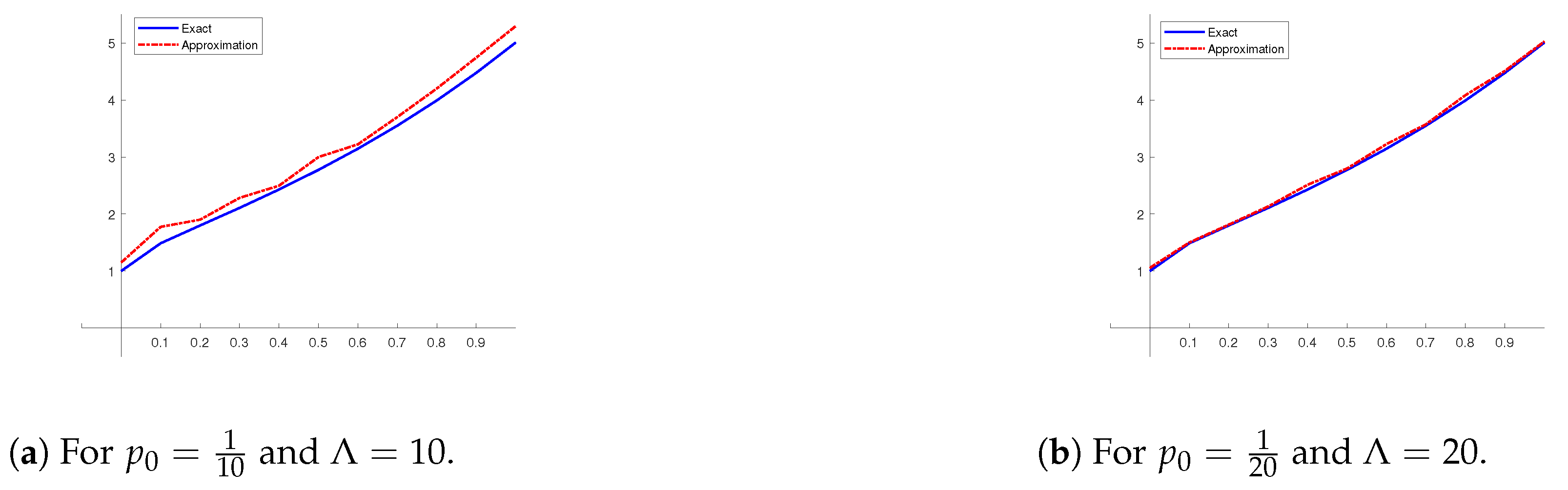
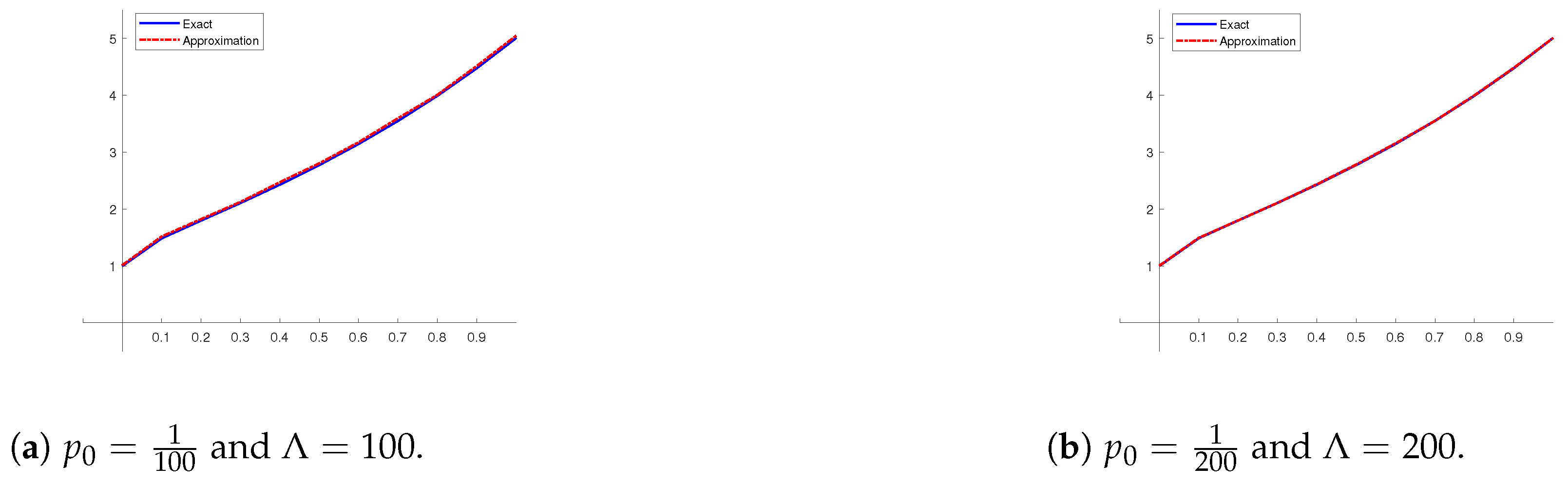
In this section, our target is to approximate the following system of difference equations:

$$\begin{array}{c}\hfill \begin{array}{cc}\hfill \left({{}_0{}^{LC}\nabla }_{p_0}^{\alpha }\mathrm{w}\right)\left(x_1\left(n{p}_0\right)\right)& =y\left(x_2\left(n{p}_0\right)\right),\hfill \\ \hfill \left({{}_0{}^{LC}\nabla }_{p_0}^{\beta }y\right)\left(n{p}_0\right)& =f\left(x_2\left(n{p}_0\right),\mathrm{w}\left(x_1\left(n{p}_0\right)\right)\right),\hfill \end{array}\end{array}$$

(18)

subject to the conditions

$$\begin{array}{c}\hfill \begin{array}{cc}\hfill \left({{}_0{}^{LC}\nabla }_{p_0}^{\alpha }\mathrm{w}\right)(-2p_0)& ={\mathrm{w}}_0,\hfill \\ \hfill \mathrm{w}(-p_0)& ={\mathrm{w}}_1,\hfill \end{array}\end{array}$$

(19)

where $\alpha ,\beta \in (0,1]$, $p_0>0$, ${\mathrm{w}}_0$ and ${\mathrm{w}}_1$ are constant vectors in $\mathbb{R}$.

Theorem 1.

System (18) with (19) has the solution

$$\begin{array}{cc}\hfill \mathrm{w}\left(x_1\left(n{p}_0\right)\right)& ={\mathrm{w}}_1+{\psi }_{2,0}\left(n{p}_0\right){\mathrm{w}}_0+\left({{}_0\nabla }_{p_0}^{-\alpha }g\right)\left(x_1\left(n{p}_0\right)\right),\hfill \end{array}$$

(20)

where $g\left(n{p}_0\right)=\left({{}_0\nabla }_{p_0}^{-\beta }F\right)\left(x_2\left(n{p}_0\right)\right)$ and $F\left(x_2\left(n{p}_0\right)\right)=f\left(x_2\left(n{p}_0\right),\mathrm{w}\left(x_1\left(n{p}_0\right)\right)\right)$, for $n\in {\mathbb{N}}_0$.

Proof. 

By considering Lemma 4 with $t=x_2\left(n{p}_0\right),x_1\left(n{p}_0\right)$, one can have

$$\begin{array}{cc}\hfill \left[{{}_0\nabla }_{p_0}^{-\beta }\left({{}_0{}^{LC}\nabla }_{p_0}^{\beta }y\right)\right]\left(x_2\left(n{p}_0\right)\right)& =y\left(x_2\left(n{p}_0\right)\right)-y\left(0\right)\hfill \\ \hfill & =\left({{}_0{}^{LC}\nabla }_{p_0}^{\alpha }\mathrm{w}\right)\left(x_1\left(n{p}_0\right)\right)-{\mathrm{w}}_0,\hfill \end{array}$$

(21)

and

$$\begin{array}{cc}\hfill \left[{{}_0\nabla }_{p_0}^{-\alpha }\left({{}_0{}^{LC}\nabla }_{p_0}^{\alpha }\mathrm{w}\right)\right]\left(x_1\left(n{p}_0\right)\right)& =\mathrm{w}\left(x_1\left(n{p}_0\right)\right)-{\mathrm{w}}_1.\hfill \end{array}$$

(22)

It follows from (21) that

$$\begin{array}{cc}\hfill \left({{}_0{}^{LC}\nabla }_{p_0}^{\alpha }\mathrm{w}\right)\left(x_1\left(n{p}_0\right)\right)& ={\mathrm{w}}_0+\left({{}_0\nabla }_{p_0}^{-\beta }F\right)\left(x_2\left(n{p}_0\right)\right),\hfill \end{array}$$

and it follows from this, Remark 2 (ii), and (22) that

$$\begin{array}{cc}\hfill \mathrm{w}\left(x_1\left(n{p}_0\right)\right)& ={\mathrm{w}}_1+\left({{}_0\nabla }_{p_0}^{-\alpha }\left[{\mathrm{w}}_0+\left({{}_0\nabla }_{p_0}^{-\beta }F\right)\left(x_2\left(n{p}_0\right)\right)\right]\right)\left(x_1\left(n{p}_0\right)\right)\hfill \\ \hfill & ={\mathrm{w}}_1+\left({{}_0\nabla }_{p_0}^{-\alpha }1\right)\left(x_1\left(n{p}_0\right)\right){\mathrm{w}}_0+\left({{}_0\nabla }_{p_0}^{-\alpha }g\right)\left(x_1\left(n{p}_0\right)\right)\hfill \\ \hfill & ={\mathrm{w}}_1+\left({\displaystyle \genfrac{}{}{0pt}{}{n-2+\alpha }{n-2}}\right){p_0}^{\alpha }{\mathrm{w}}_0+\left({{}_0\nabla }_{p_0}^{-\alpha }g\right)\left(n{p}_0\right)\hfill \\ \hfill & ={\mathrm{w}}_1+{\psi }_{2,0}\left(n{p}_0\right){\mathrm{w}}_0+\left({{}_0\nabla }_{p_0}^{-\alpha }g\right)\left(x_1\left(n{p}_0\right)\right),\hfill \end{array}$$

where $g\left(n{p}_0\right)=\left({{}_0\nabla }_{p_0}^{-\beta }F\right)\left(x_2\left(n{p}_0\right)\right)$ and $F\left(x_2\left(n{p}_0\right)\right)=f\left(x_2\left(n{p}_0\right),\mathrm{w}\left(x_1\left(n{p}_0\right)\right)\right)$, for $n\in {\mathbb{N}}_0$. Hence, the proof is completed. □

Remark 3.

Following [42] [Theorem 4.1], we can deduce that system (18) has a unique solution (i.e., (20) is unique) such that y and f satisfy the Lipschitz condition, i.e.,

$$\begin{array}{c}\hfill \left|y\left(n_1\right)-y\left(n_2\right)\right|\le L_1\left|n_1-n_2\right|,\end{array}$$

and

$$\begin{array}{c}\hfill \left|f(n,\mathrm{w})-f(n_2,\tilde{\mathrm{w}})\right|\le L_2\left|\mathrm{w}-\tilde{\mathrm{w}}\right|,\end{array}$$

for some positive constant $L_1$ and $L_2$.

In the following theorem, we examine the solution of a particular case of system (18).

Theorem 2.

Systems (18) and (19) have the following solution:

$$\begin{array}{cc}\hfill \mathrm{w}\left(x_1\left(n{p}_0\right)\right)& =\sum _{\kappa =0}^{\infty }{A}^{\kappa }\left({\psi }_{\kappa ,\kappa }{\mathrm{w}}_1+{\psi }_{\kappa +2,\kappa }{\mathrm{w}}_0\right)\left(n{p}_0\right),\hfill \end{array}$$

(23)

where $f\left(x_1\left(n{p}_0\right),\mathrm{w}\left(x_1\left(n{p}_0\right)\right)\right)=A\mathrm{w}\left(x_1\left(n{p}_0\right)\right)$, and $n\in {\mathbb{N}}_0$.

Proof. 

First, we try to investigate (23). In the case of $n=0$, it follows from (20) that

$$\begin{array}{cc}\hfill \mathrm{w}(-p_0)& ={\mathrm{w}}_1+{\psi }_{2,0}\left(0\right){\mathrm{w}}_0+\left({{}_0\nabla }_{p_0}^{-\alpha }g\right)(-p_0)={\mathrm{w}}_1,\hfill \end{array}$$

which is equivalent to

$$\begin{array}{cc}\hfill \mathrm{w}(-p_0)& =\left({\psi }_{0,0}{\mathrm{w}}_1+{\psi }_{2,0}{\mathrm{w}}_0\right)\left(0\right)+\underset{=0}{\underbrace{\sum _{\kappa =1}^{\infty }{A}^{\kappa }\left({\psi }_{\kappa ,\kappa }{\mathrm{w}}_1+{\psi }_{\kappa +1,\kappa }{\mathrm{w}}_0\right)\left(0\right)}},\hfill \end{array}$$

according to Remark 2 (vi) and the convention that

$$\begin{array}{cc}\hfill \left({{}_0\nabla }_{p_0}^{-\alpha }g\right)(-p_0)& ={\displaystyle \frac{p_0}{\Gamma \left(\alpha \right)}}\sum _{r=1}^{-1}{\left(-r{p}_0\right)}_{p_0}^{\overline{\alpha -1}}g\left(r{p}_0\right)=0.\hfill \end{array}$$

Next, for $n>0$, we define

$$\begin{array}{cc}\hfill {\mathrm{w}}_{m+1}\left(x_1\left(n{p}_0\right)\right)& ={\psi }_{0,0}\left(n{p}_0\right){\mathrm{w}}_1+{\psi }_{2,0}\left(n{p}_0\right){\mathrm{w}}_0+\left({{}_0\nabla }_{p_0}^{-\alpha }{g}_m\right)\left(n{p}_0\right),\hfill \end{array}$$

where $g_m\left(n{p}_0\right)=\left({{}_0\nabla }_{p_0}^{-\beta }{F}_m\right)\left(x_2\left(n{p}_0\right)\right)$ and $F_m\left(x_2\left(n{p}_0\right)\right)=A{\mathrm{w}}_m\left(x_1\left(n{p}_0\right)\right)$, for $m\in {\mathbb{N}}_0$.

Then, we see that

$$\begin{array}{cc}\hfill {\mathrm{w}}_1\left(x_1\left(n{p}_0\right)\right)& ={\psi }_{0,0}\left(n{p}_0\right){\mathrm{w}}_1+{\psi }_{2,0}\left(n{p}_0\right){\mathrm{w}}_0+\left({{}_0\nabla }_{p_0}^{-\alpha }{g}_0\right)\left(x_1\left(n{p}_0\right)\right)\hfill \\ \hfill & ={\psi }_{0,0}\left(n{p}_0\right){\mathrm{w}}_1+{\psi }_{2,0}\left(n{p}_0\right){\mathrm{w}}_0\hfill \\ \hfill & +A{\mathrm{w}}_1\left[{{}_0\nabla }_{p_0}^{-\alpha }\left({{}_0\nabla }_{p_0}^{-\beta }1\right)\left(n{p}_0\right)\right]\left(x_1\left(n{p}_0\right)\right)\hfill \\ \hfill & ={\psi }_{0,0}\left(n{p}_0\right){\mathrm{w}}_1+{\psi }_{2,0}\left(n{p}_0\right){\mathrm{w}}_0+A{\mathrm{w}}_1\left({{}_0\nabla }_{p_0}^{-\alpha }{\psi }_{0,1}\right)\left(x_1\left(n{p}_0\right)\right)\hfill \\ \hfill & ={\psi }_{0,0}\left(n{p}_0\right){\mathrm{w}}_1+{\psi }_{2,0}\left(n{p}_0\right){\mathrm{w}}_0+A{\psi }_{1,1}\left(n{p}_0\right){\mathrm{w}}_1,\hfill \end{array}$$

where we use Remark 2 (iii), (v), and

$$\begin{array}{cc}\hfill g_0\left(n{p}_0\right)=\left({{}_0\nabla }_{p_0}^{-\beta }{F}_0\right)\left(x_2\left(n{p}_0\right)\right)& =A{\mathrm{w}}_0\left(x_1\left(n{p}_0\right)\right)\left({{}_0\nabla }_{p_0}^{-\beta }1\right)\left(x_2\left(n{p}_0\right)\right)\hfill \\ \hfill & =A{\mathrm{w}}_1{\psi }_{0,1}\left(n{p}_0\right).\hfill \end{array}$$

Using the same technique together with using Remark 2 (iii) and (v), we can deduce

$$\begin{array}{c}{\mathrm{w}}_2\left(x_1\left(n{p}_0\right)\right)={\psi }_{0,0}\left(n{p}_0\right){\mathrm{w}}_1+{\psi }_{2,0}\left(n{p}_0\right){\mathrm{w}}_0+\left({{}_0\nabla }_{p_0}^{-\alpha }{g}_1\right)\left(x_1\left(n{p}_0\right)\right)\hfill \\ ={\psi }_{0,0}\left(n{p}_0\right){\mathrm{w}}_1+{\psi }_{2,0}\left(n{p}_0\right){\mathrm{w}}_0+A\left[{\psi }_{1,1}\left(n{p}_0\right){\mathrm{w}}_1+{\psi }_{3,1}\left(n{p}_0\right){\mathrm{w}}_0\right]\\ \hfill +A^2{\psi }_{2,2}\left(n{p}_0\right){\mathrm{w}}_1,\end{array}$$

where

$$\begin{array}{cc}\hfill g_1\left(n{p}_0\right)& =\left({{}_0\nabla }_{p_0}^{-\beta }{F}_1\right)\left(x_2\left(n{p}_0\right)\right)\hfill \\ \hfill & =A\left[{\mathrm{w}}_1\left({{}_0\nabla }_{p_0}^{-\beta }{\psi }_{0,0}\right)\left(n{p}_0\right)+{\mathrm{w}}_0\left({{}_0\nabla }_{p_0}^{-\beta }{\psi }_{2,0}\right)\left(n{p}_0\right)+A{\mathrm{w}}_1\left({{}_0\nabla }_{p_0}^{-\beta }{\psi }_{1,1}\right)\left(n{p}_0\right)\right]\hfill \\ \hfill & =A\left[{\psi }_{0,1}\left(n{p}_0\right){\mathrm{w}}_1+{\psi }_{2,1}\left(n{p}_0\right){\mathrm{w}}_0+A{\psi }_{1,2}\left(n{p}_0\right){\mathrm{w}}_1\right].\hfill \end{array}$$

By the same process, we can obtain the desired result in (23). □

The following lemmas are useful to obtain our main result.

Lemma 5.

If $0<\alpha \le 1$, then the following summation formula can be obtained:

$$\begin{array}{c}\hfill \underset{p_0\to 0}{lim}{\left(t_{p_0}-a\right)}^{\overline{-\alpha }}={(t-a)}^{-\alpha },\end{array}$$

for $p_0>0$, $t>a$, where $a\in \mathbb{R}$, $t_{p_0}=a+p_0+n{p}_0$, and $n=\left[{\displaystyle \frac{t-a}{p_0}}\right]+1$.

Proof. 

Consider

$$\begin{array}{cc}\hfill {\left(t_{p_0}-a\right)}^{\overline{-\alpha }}& ={\displaystyle \frac{\Gamma (n+1-\alpha )}{\Gamma (n+1)}}{p_0}^{-\alpha }\hfill \\ \hfill & ={\displaystyle \frac{\Gamma (n+1-\alpha )}{\Gamma (n+1)}}{\left(t_{p_0}-a\right)}^{-\alpha }{(n+1)}^{\alpha }.\hfill \end{array}$$

As $p_0\to 0$ (or $n\to \infty$), it follows that

$$\begin{array}{cc}\hfill \underset{p_0\to 0}{lim}{\left(t_{p_0}-a\right)}^{\overline{-\alpha }}& =\underset{p_0\to 0}{lim}{\displaystyle \frac{\Gamma (n+1-\alpha )}{\Gamma (n+1)}}{\left(t_{p_0}-a\right)}^{-\alpha }{(n+1)}^{\alpha }\hfill \\ \hfill & =\underset{p_0\to 0}{lim}{\left(t_{p_0}-a\right)}^{-\alpha }·\underset{n\to \infty }{lim}{\displaystyle \frac{\Gamma (n+1-\alpha )}{\Gamma (n+1)}}{(n+1)}^{\alpha }\hfill \\ \hfill & \approx {(t-a)}^{-\alpha },\hfill \end{array}$$

where it is seen that

$$\begin{array}{c}\hfill \underset{p_0\to 0}{lim}\left(t_{p_0}-a\right)=\underset{p_0\to 0}{lim}\left(p_0+(t-a)+p_0\right)=t-a,\end{array}$$

and the asymptotic formula is (see [39])

$$\begin{array}{c}\hfill \underset{n\to \infty }{lim}{\displaystyle \frac{\Gamma (n+1-\alpha )}{\Gamma (n+1)}}{(n+1)}^{\alpha }=1+O\left({\displaystyle \frac{1}{n+1}}\right)\approx 1.\end{array}$$

(24)

This proves the result. □

Lemma 6.

If $\alpha \in (0,1]$, then the following summation formula holds:

$$\begin{array}{cc}\hfill \left({{}_a{}^{RL}\nabla }_{p_0}^{\alpha }\mathrm{w}\right)\left(t_{p_0}\right)& ={p_0}^{-\alpha }\sum _{j=0}^n{(-1)}^j\left({\displaystyle \genfrac{}{}{0pt}{}{\alpha }{j}}\right)\mathrm{w}\left(t_{p_0}-j{p}_0\right),\hfill \end{array}$$

(25)

for $t>a$ and $p_0>0$ with $a\in \mathbb{R}$, $t_{p_0}=a+p_0+n{p}_0$, and $n\in {\mathbb{N}}_0$.

Proof. 

Considering Definition (8), one can have

$$\begin{array}{cc}\hfill \left({{}_a{}^{RL}\nabla }_{p_0}^{\alpha }\mathrm{w}\right)\left(t_{p_0}\right)& ={\displaystyle \frac{1}{\Gamma (-\alpha )}}\sum _{m=0}^{{\displaystyle \frac{t-a}{p_0}}-1}{\left(t_{p_0}-a-m{p}_0\right)}_{p_0}^{\overline{-\alpha -1}}{p}_0\mathrm{w}(a+p_0+m{p}_0)\hfill \\ \hfill & =p_0\sum _{m=0}^n{\displaystyle \frac{{\left(n{p}_0+p_0-m{p}_0\right)}_{p_0}^{\overline{-\alpha -1}}}{\Gamma (-\alpha )}}\mathrm{w}(a+p_0+m{p}_0)\hfill \\ \hfill & ={p_0}^{-\alpha }\sum _{m=0}^n{\displaystyle \frac{\Gamma (n-m-\alpha )}{\Gamma (n-m+1)\Gamma (-\alpha )}}\mathrm{w}(a+p_0+m{p}_0)\hfill \\ \hfill & ={p_0}^{-\alpha }\sum _{m=0}^n\left({\displaystyle \genfrac{}{}{0pt}{}{n-m-\alpha -1}{n-m}}\right)\mathrm{w}(a+p_0+m{p}_0)\hfill \\ \hfill & ={p_0}^{-\alpha }\sum _{j=0}^n\left({\displaystyle \genfrac{}{}{0pt}{}{j-\alpha -1}{j}}\right)\mathrm{w}(a+x_2\left(n{p}_0\right)-j{p}_0)\hfill \\ \hfill & ={p_0}^{-\alpha }\sum _{j=0}^n{(-1)}^j\left({\displaystyle \genfrac{}{}{0pt}{}{\alpha }{j}}\right)\mathrm{w}(a+x_2\left(n{p}_0\right)-j{p}_0)\hfill \\ \hfill & ={p_0}^{-\alpha }\sum _{j=0}^n{(-1)}^j\left({\displaystyle \genfrac{}{}{0pt}{}{\alpha }{j}}\right)\mathrm{w}(t_{p_0}-j{p}_0),\hfill \end{array}$$

where we used (6). Thus, the proof is completed. □

Theorem 3.

If $0<\alpha \le 1$, $\mathrm{w}$ is a continuous function, and ${\mathrm{w}}^{\prime }$ is integrable on $[a,\Lambda ]$ with $\Lambda >0$, then, for $p_0>0$ and $t>a$ with $a\in \mathbb{R}$, one can have

$$\begin{array}{cc}\hfill \left({{}_a{}^{LC}D}^{\alpha }\mathrm{w}\right)\left(t\right)& =\underset{p_0\to 0}{lim}\left({{}_a{}^{LC}\nabla }_{p_0}^{\alpha }\mathrm{w}\right)\left(t_{p_0}\right),\hfill \end{array}$$

where $t_{p_0}=a+p_0+n{p}_0$ and $n\in {\mathbb{N}}_0$.

Proof. 

By using (25) in (11), we can deduce

$$\begin{array}{cc}\hfill \left({{}_a{}^{LC}\nabla }_{p_0}^{\alpha }\mathrm{w}\right)\left(t_{p_0}\right)& ={p_0}^{-\alpha }\sum _{j=0}^n{(-1)}^j\left({\displaystyle \genfrac{}{}{0pt}{}{\alpha }{j}}\right)\mathrm{w}\left(t_{p_0}-j{p}_0\right)-{\displaystyle \frac{{\left(t_{p_0}-a\right)}_{p_0}^{\overline{-\alpha }}}{\Gamma (1-\alpha )}}\mathrm{w}\left(a\right),\hfill \end{array}$$

(26)

for $t_{p_0}=a+p_0+n{p}_0$. As $p_0\to 0$ on both sides of (26), we obtain the result by using Lemma 5. □

Proposition 1.

If $\alpha \in (0,1]$ and $p_0>0$, then the solution of

$$\begin{array}{cc}\hfill \left({{}_0{}^{LC}D}^{\alpha }\mathrm{w}\right)\left(t\right)& =f\left(t,\mathrm{w}(t\right),\hfill \\ \hfill & \mathrm{w}\left(0\right)={\mathrm{w}}_0,\hfill \end{array}$$

can be estimated with the solution of

$$\begin{array}{cc}\hfill \left({{}_a{}^{LC}\nabla }^{\alpha }\tilde{\mathrm{w}}\right)\left(t\right)& =f\left(t,\tilde{\mathrm{w}}\left(t\right)\right),\hfill \\ \hfill \tilde{\mathrm{w}}\left(a\right)& ={\mathrm{w}}_0,\hfill \end{array}$$

via the following limit:

$$\begin{array}{c}\hfill \underset{p_0\to 0}{lim}\tilde{\mathrm{w}}\left(t_{p_0}\right)=\mathrm{w}\left(t\right),\end{array}$$

where $t_{p_0}=a+p_0+n{p}_0$ and $n=\left[(t-p_0)/p_0\right]+1$.

Proposition 2.

If $\alpha \in (0,1]$ and $p_0>0$, then the solution of

$$\begin{array}{cc}\hfill \left[{{}_0{}^{LC}D}^{\beta }\left({{}_0{}^{LC}D}^{\alpha }\mathrm{w}\right)\right]\left(t\right)& =f\left(t,\mathrm{w}\left(t\right)\right),\hfill \\ \hfill & \mathrm{w}\left(0\right)={\mathrm{w}}_0,\hfill \end{array}$$

can be approximated with the solutions of (18) and (19) via the limit

$$\begin{array}{c}\hfill \underset{p_0\to 0}{lim}\tilde{\mathrm{w}}\left(t_{p_0}\right)=\mathrm{w}\left(t\right),\end{array}$$

where n and $t_{p_0}$ are given in Proposition 1.

4. Numerical Tests

In this section, we will present the result of the numerical experiment in [40] to demonstrate the effectiveness of the proposed technique.

For this reason, we consider

$$\begin{array}{cc}\hfill & \left({{}_0{}^{LC}D}^{\alpha }\mathrm{w}\right)\left(t\right)=\mathrm{w}\left(t\right)\mathrm{with}\mathrm{w}\left(0\right)=1,\hfill \end{array}$$

where its solution is given in [40] by

$$\begin{array}{c}\hfill \mathrm{w}\left(t\right)=E\left(t^{\alpha }\right):=\sum _{\kappa =0}^{\infty }{\displaystyle \frac{t^{\alpha \kappa }}{\Gamma (\alpha \kappa +1)}}.\end{array}$$

To compare the efficiency of the methods, we report, in Figure 1 and Figure 2, the actual computational results ($\mathrm{w}$) compared with the numerical results ($\tilde{\mathrm{w}}$) in the cases of $\alpha ={\displaystyle \frac{1}{2}}$ and $t=0,0.1,\dots ,1$ for different values of $p_0$ and $\Lambda$.

Furthermore, we know that

$$\begin{array}{cc}\hfill \left[{{}_0{}^{LC}D}^{\alpha }\left({{}_0{}^{LC}D}^{\alpha }\mathrm{w}\right)\right]\left(t\right)& =\mathrm{w}\left(t\right),\hfill \\ \hfill \left({{}_0{}^{LC}D}^{\alpha }\mathrm{w}\right)\left(0\right)& =1,\hfill \\ \hfill \mathrm{w}\left(0\right)& =1,\hfill \end{array}$$

where its exact solution is $\mathrm{w}\left(t\right)=E\left(t^{\alpha }\right)$.

As a result, by considering Figure 1 and Figure 2 and

Table 1. Numerical results in case of $p_0=0.1$.

$\mathit{E}\left({\mathit{t}}^{\frac{1}{2}}\right)$	Numerical Result	$\left|\mathbf{Error}\right|$
1.000000000000000	1.003804458469754	0.003804458469754
1.486763397673679	1.492441614080931	0.005678216407252
1.799017244188177	1.799775787083807	0.000758542895631
2.107699203837270	2.108238705023936	0.000539501186666
2.430043141497662	2.435351117027752	0.005307975530090
2.774285957670009	2.782077629971030	0.007791672301020
3.146213032210335	3.155553139052627	0.009340106842292
3.550802683646889	3.552101745731627	0.001299062084737
3.992835834192708	3.998524070801430	0.005688236608722
4.477184810795735	4.481878717206317	0.004693906410582
5.008980080762283	5.009099101457296	0.000119020695013

and

Table 2. Numerical results in case of $p_0=0.01$.

$\mathit{E}\left({\mathit{t}}^{\frac{1}{2}}\right)$	Numerical Result	$\left|\mathbf{Error}\right|$
1.000000000000000	1.000711215780434	0.000711215780434
1.486763397673679	1.486985144407696	0.000221746734017
1.799017244188177	1.799134661839032	0.000117417650856
2.107699203837270	2.107995879710488	0.000296675873218
2.430043141497662	2.430361919799588	0.000318778301926
2.774285957670009	2.774710124429723	0.000424166759714
3.146213032210335	3.146720890494996	0.000507858284661
3.550802683646889	3.550888199443980	0.000085515797090
3.992835834192708	3.993098316427406	0.000262482234698
4.477184810795735	4.477985825418505	0.000801014622770
5.008980080762283	5.009009301039845	0.000029220277562

, we conclude that the exact solution can be obtained from $\tilde{\mathrm{w}}$ such that $p_0$ is sufficiently small. This implies the applicability of Theorem 3 where $p_0\to 0$.

5. Concluding Remarks and Future Works

To summarize, we investigated the complete solution of a sequential fractional differential problem of Liouville–Caputo type including certain initial value conditions,

$$\begin{array}{cc}\hfill \left[{{}_0{}^{LC}D}^{\beta }\left({{}_0{}^{LC}D}^{\alpha }\mathrm{w}\right)\right]\left(t\right)& =f\left(t,\mathrm{w}\left(t\right)\right),\hfill \end{array}$$

with the condition $\mathrm{w}\left(0\right)={\mathrm{w}}_1$, by analyzing the corresponding system of the fractional difference,

$$\begin{array}{cc}\hfill \left({{}_0{}^{LC}\nabla }_{p_0}^{\alpha }\tilde{\mathrm{w}}\right)\left(x_1\left(n{p}_0\right)\right)& =y\left(x_2\left(n{p}_0\right)\right),\hfill \\ \hfill \left({{}_0{}^{LC}\nabla }_{p_0}^{\alpha }y\right)(nh+h)& =f\left(x_1\left(n{p}_0\right),\tilde{\mathrm{w}}\left(x_1\left(n{p}_0\right)\right)\right),\hfill \end{array}$$

subject to the conditions

$$\begin{array}{cc}\hfill \left({{}_0{}^{LC}\nabla }_{p_0}^{\alpha }\tilde{\mathrm{w}}\right)(-p_0)& ={\tilde{\mathrm{w}}}_0,\hfill \\ \hfill \tilde{\mathrm{w}}(-2p_0)& ={\tilde{\mathrm{w}}}_a,\hfill \end{array}$$

via the following limitation:

$$\begin{array}{c}\hfill \underset{p_0\to 0}{lim}\tilde{\mathrm{w}}\left(t_{p_0}\right)=\mathrm{w}\left(t\right),\end{array}$$

where $t_{p_0}$ and n are defined in Proposition 1. We used the expressions ${\psi }_{\kappa ,s}$ and ${\tilde{\psi }}_{\kappa ,s}$ in the solution of the discrete fractional difference system as stated in Definition 4.

Furthermore, the numerical example shows that the new reconstruction method can obtain a very high order of accuracy; when the value of $p_0$ is small enough (or $\Lambda$ is large enough), the approximation results are in good agreement with the exact one.

Concerning future works, we plan to extend the numerical schemes presented here to apply them to other types of discrete fractional systems including exponential and Mittag–Leffler systems in kernels to establish similar results (visit [22,38] to see these operators).

References

1. Kilbas, A.A.; Srivastava, H.M.; Trujillo, J.J. Theory and Applications of Fractional Differential Equations; Elsevier B.V.: Amsterdam, The Netherlands, 2006. [Google Scholar]
2. Cinar, M.; Secer, A.; Ozisik, M.; Bayram, M. Derivation of optical solitons of dimensionless Fokas-Lenells equation with perturbation term using Sardar sub-equation method. Opt. Quant. Electron 2022, 54, 402. [Google Scholar]
3. Ehsan, H.; Abbas, M.; Nazir, T.; Mohammed, P.O.; Chorfi, N.; Baleanu, D. Efficient analytical algorithms to study Fokas dynamical models involving M-truncated derivative. Qual. Theory Dyn. Syst. 2024, 23, 49. [Google Scholar]
4. Dos Santos, J.P.C.; Arjunan, M.M.; Cuevas, C. Existence results for fractional neutral integro-differential equations with state-dependent delay. Comput. Math. Appl. 2011, 62, 1275–1283. [Google Scholar]
5. Goodrich, C.S.; Peterson, A.C. Discrete Fractional Calculus; Springer: Berlin/Heidelberg, Germany, 2015. [Google Scholar]
6. Korpinar, Z.; Inc, M.; Baleanu, D.; Bayram, M. Theory and application for the time fractional Gardner equation with Mittag-Leffler kernel. J. Taibah Univ. Sci. 2019, 13, 813–819. [Google Scholar]
7. Hashemi, M.S.; Inc, M.; Bayram, M. Symmetry properties and exact solutions of the time fractional Kolmogorov-Petrovskii-Piskunov equation. Rev. Mex. Física 2019, 65, 529–535. [Google Scholar]
8. Chadha, A.; Pandey, D.N. Existence of mild solutions for a fractional equation with state-dependent delay via resolvent operators. Nonlinear Stud. 2015, 22, 71–85. [Google Scholar]
9. Phuong, N.D.; Sakar, F.M.; Etemad, S.; Rezapour, S. A novel fractional structure of a multi-order quantum multi-integro-differential problem. Adv. Differ. Equ. 2020, 2020, 633. [Google Scholar]
10. Rezapour, S.; Imran, A.; Hussain, A.; Martínez, F.; Etemad, S.; Kaabar, M.K.A. Condensing Functions and Approximate Endpoint Criterion for the Existence Analysis of Quantum Integro-Difference FBVPs. Symmetry 2021, 13, 469. [Google Scholar] [CrossRef]
11. Etemad, S.; Matar, M.M.; Ragusa, M.A.; Rezapour, S. Tripled Fixed Points and Existence Study to a Tripled Impulsive Fractional Differential System via Measures of Noncompactness. Mathematics 2022, 10, 25. [Google Scholar]
12. Atici, F.; Uyanik, M. Analysis of discrete fractional operators. Appl. Anal. Discret. Math. 2015, 9, 139–149. [Google Scholar]
13. Atici, F.M.; Atici, M.; Belcher, M.; Marshall, D. A new approach for modeling with discrete fractional equations. Fund. Inform. 2017, 151, 313–324. [Google Scholar]
14. Atici, F.; Sengul, S. Modeling with discrete fractional equations. J. Math. Anal. Appl. 2010, 369, 1–9. [Google Scholar]
15. Goodrich, C.S. On discrete sequential fractional boundary value problems. J. Math. Anal. Appl. 2012, 385, 111–124. [Google Scholar]
16. Noureen, R.; Naeem, M.N.; Baleanu, D.; Mohammed, P.O.; Almusawa, M.Y. Application of trigonometric B-spline functions for solving Caputo time fractional gas dynamics equation. AIMS Math. 2023, 8, 25343–25370. [Google Scholar]
17. Silem, A.; Wu, H.; Zhang, D.-J. Discrete rogue waves and blow-up from solitons of a nonisospectral semi-discrete nonlinear Schrödinger equation. Appl. Math. Lett. 2021, 116, 107049. [Google Scholar]
18. Liu, Y.; Liu, H.; Zhu, Y. An approach for numerical solutions of Caputo-Hadamard uncertain fractional differential equations. Fractal Fract. 2022, 6, 693. [Google Scholar] [CrossRef]
19. Lu, Q.; Zhu, Y. Comparison theorems and distributions of solutions to uncertain fractional difference equations. J. Comput. Appl. Math. 2020, 376, 112884. [Google Scholar]
20. Chen, C.R.; Bohner, M.; Jia, B.G. Ulam-Hyers stability of Caputo fractional difference equations. Math. Meth. Appl. Sci. 2019, 42, 7461–7470. [Google Scholar]
21. Lizama, C. The Poisson distribution, abstract fractional difference equations, and stability. Proc. Am. Math. Soc. 2017, 145, 3809–3827. [Google Scholar]
22. Mohammed, P.O.; Abdeljawad, T.; Hamasalh, F.K. On discrete delta Caputo-Fabrizio fractional operators and monotonicity analysis. Fractal Fract. 2021, 5, 116. [Google Scholar] [CrossRef]
23. Liu, X.; Du, F.; Anderson, D.; Jia, B. Monotonicity results for nabla fractional h-difference operators. Math. Meth. Appl. Sci. 2021, 44, 1207–1218. [Google Scholar]
24. Abdeljawad, T.; Baleanu, D. Monotonicity analysis of a nabla discrete fractional operator with discrete Mittag-Leffler kernel. Chaos Solit. Fractals 2017, 116, 1–5. [Google Scholar]
25. Goodrich, C.S.; Lizama, C. Positivity, monotonicity, and convexity for convolution operators. Discret. Contin. Dyn. Syst. 2020, 40, 4961–4983. [Google Scholar]
26. Wu, G.-C.; Baleanu, D.; Zeng, S.-D. Discrete chaos in fractional sine and standard maps. Phys. Lett. A 2014, 378, 484–487. [Google Scholar]
27. He, J.W.; Zhang, L.; Zhou, Y.; Ahmad, B. Existence of solutions for fractional difference equations via topological degree methods. Adv. Differ. Equ. 2018, 2018, 153. [Google Scholar]
28. Huang, L.-L.; Park, J.H.; Wu, G.-C.; Mo, Z.-W. Variable-order fractional discrete-time recurrent neural networks. J. Comput. Appl. Math. 2020, 370, 112633. [Google Scholar]
29. Mohammed, P.O.; Baleanu, D.; Al-Sarairah, E.; Abdeljawad, T.; Chorfi, N. Theoretical and numerical computations of convexity analysis for fractional differences using lower boundedness. Fractals 2023, 31, 2340183. [Google Scholar]
30. Mohammed, P.O.; Almusawa, M.Y. On analysing discrete sequential operators of fractional order and their monotonicity results. AIMS Math. 2023, 8, 12872–12888. [Google Scholar]
31. Segi Rahmat, M.R.; Md Noorani, M.S. Caputo type fractional difference operator and its application on discrete time scales. Adv. Differ. Equ. 2015, 2015, 160. [Google Scholar]
32. Almusawa, M.Y.; Mohammed, P.O. Approximation of sequential fractional systems of Liouville-Caputo type by discrete delta difference operators. Chaos Solit. Fractals 2023, 176, 114098. [Google Scholar]
33. Fečkan, M.; Pospíšil, M.; Danca, M.-F.; Wang, J. Caputo delta weakly fractional difference equations. Fract. Calc. Appl. Anal. 2022, 25, 2222–2240. [Google Scholar]
34. Srivastava, H.M.; Mohammed, P.O.; Ryoo, C.S.; Hamed, Y.S. Existence and uniqueness of a class of uncertain Liouville-Caputo fractional difference equations. J. King Saud Univ. Sci. 2021, 33, 101497. [Google Scholar]
35. Mohammed, P.O.; Goodrich, C.S.; Srivastava, H.M.; Al-Sarairah, E.; Hamed, Y.S. A study of monotonicity analysis for the delta and nabla discrete fractional operators of the Liouville-Caputo family. Axioms 2023, 12, 114. [Google Scholar] [CrossRef]
36. Mozyrska, D.; Girejko, E. Overview of Fractional h-difference Operators. In Advances in Harmonic Analysis and Operator Theory. Operator Theory: Advances and Applications; Almeida, A., Castro, L., Speck, F.O., Eds.; Birkhäuser: Basel, Switzerland, 2013; Volume 229. [Google Scholar]
37. Mozyrska, D.; Girejko, E.; Wyrwas, M. Fractional nonlinear systems with sequential operators. Cent. Eur. J. Phys. 2013, 11, 1295–1303. [Google Scholar]
38. Abdeljawad, T. Different type kernel h-fractional differences and their fractional h–sums. Chaos Solit. Fractals 2018, 116, 146–156. [Google Scholar]
39. Podlubny, I. Fractional Differential Equations; AP: New York, NY, USA, 1999. [Google Scholar]
40. Miller, K.S.; Ross, B. An Introduction to the Fractional Calculus and Fractional Differential Equation; John Wiley & Sons: New York, NY, USA, 1993. [Google Scholar]
41. Girejko, E.; Mozyrska, D. Positivity of fractional discrete systems with sequential h-differences. In Proceedings of the 2012 IEEE 4th International Conference on Nonlinear Science and Complexity (NSC), Budapest, Hungary, 6–11 August 2012; pp. 137–140. [Google Scholar]
42. Wang, M.; Jia, B.; Chen, C.; Zhu, X.; Du, F. Discrete fractional Bihari inequality and uniqueness theorem of solutions of nabla fractional difference equations with non-Lipschitz nonlinearities. Appl. Math. Comput. 2020, 367, 125118. [Google Scholar]
Figure 1. Numerical results for different values of p 0 .
Axioms 13 00570 g001
Figure 2. Numerical results for different values of p 0 .
Axioms 13 00570 g002