
Estimation of the Reliability Function of the Generalized Rayleigh Distribution under Progressive First-Failure Censoring Model

Abstract
1. Introduction
1.1. Progressive First-Failure Censoring (PFFC) Model
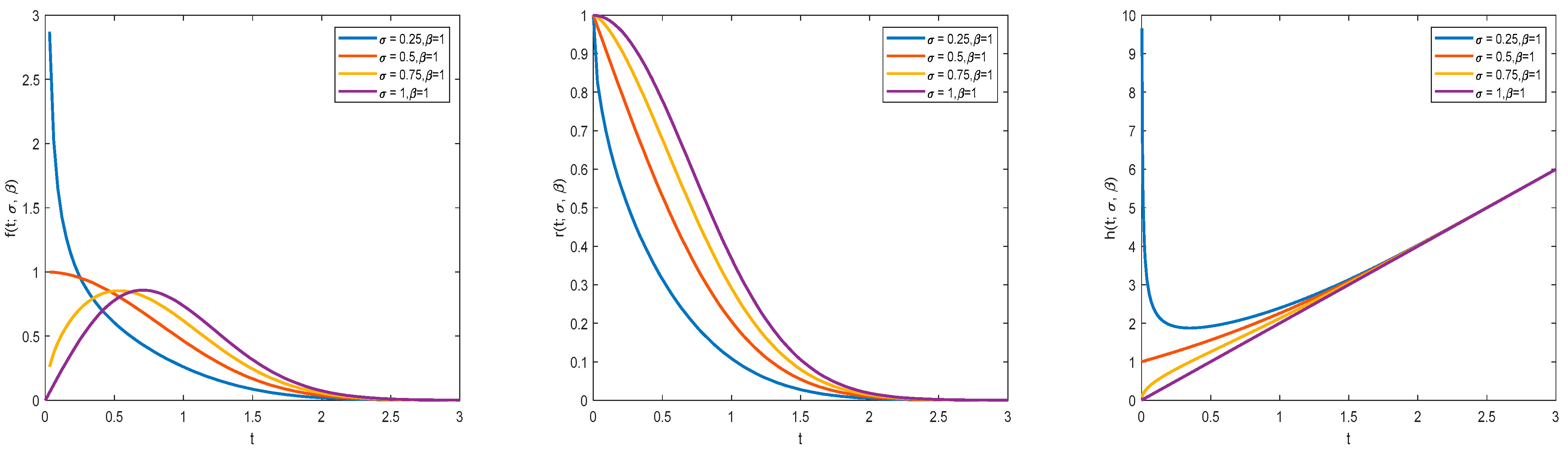
1.2. Generalized Rayleigh Distribution (GRD) Model
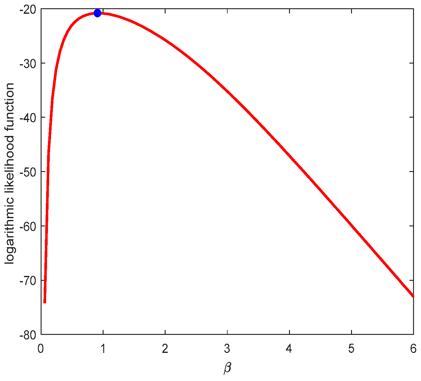
2. ML Estimation
2.1. Existence and Uniqueness of ML Estimation Solutions
2.2. EM Algorithm
3. Bootstrap CI
4. BE under Different Loss Functions
4.1. Information Prior and Non-Information Prior
- (i)
- SELF:
- (ii)
- GELF:
- (iii)
- WSELF:
- (iv)
- KLF:
- (v)
- M/Q SELF:
- (vi)
- PLF:
4.2. MCMC Method with Hybrid Gibbs Sampling
- (i)
- Select a candidate point from . If , resample until a valid candidate is obtained. Calculate the acceptance probability based on the candidate point:
- (ii)
- Generate a random number from a uniform distribution U (0, 1). Use the following formula to make the extraction:
- (iii)
- Set j = j + 1 and return to step (i) to continue repeating the above steps.
- (i)
- Select a candidate point from . If , resample until a valid candidate is obtained. Calculate the acceptance probability based on the candidate point:
- (ii)
- Generate a random number from a uniform distribution U (0, 1). Use the following equation to draw the sample:
- (iii)
- Set j = j + 1 and return to step (i) to continue repeating the above steps.
5. Monte Carlo Simulation
- (1)
- In ML estimation, the overall performance of the NR method is superior to that of the EM algorithm.
- (2)
- With the increase in sample size, the accuracy of point estimation and interval estimation improves under various estimation methods.
- (3)
- Based on parameters, RF, and HF under GRD, BE generally outperforms ML estimation.
- (4)
- In BE, the performance of information prior based BE is superior to that of non-information prior based BE.
- (5)
- In most cases, the MSE of estimated results obtained by the PFFC method with k = 2 and k = 3 is similar.
- (6)
- Under the MCMC sampling method, Bayesian estimator performs better based on PLF compared to other loss functions. However, it performs worst when based on M/Q SELF.
- (7)
- Generally speaking, censoring scheme c has superior performance and yields better results compared to the other two censoring schemes.
- (8)
- As sample size increases, AW for different CIs shows a decreasing trend. The AW for Boot-t CI is greater than that for Bayesian Cred.CI. When k = 3, AW for all CIs performs best.
- (9)
- Under conditions with informative prior available, AW for Bayesian Cred.CIs is smaller than that non-information prior available.
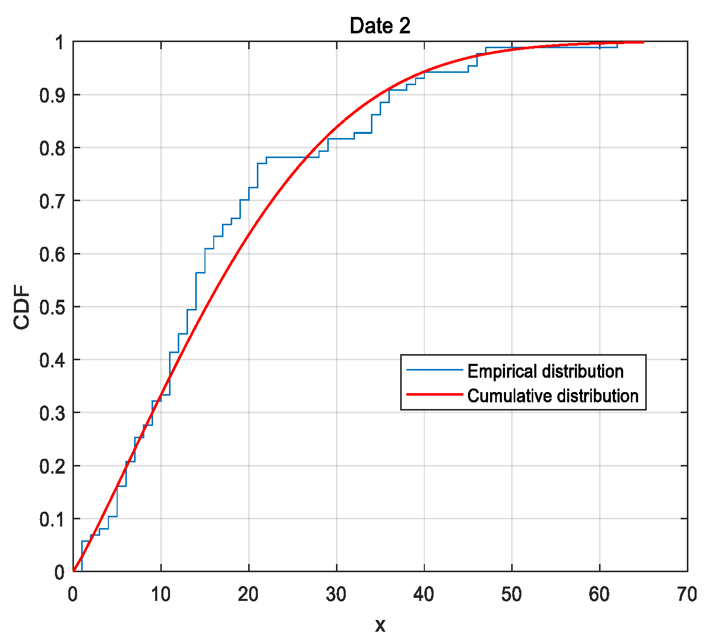
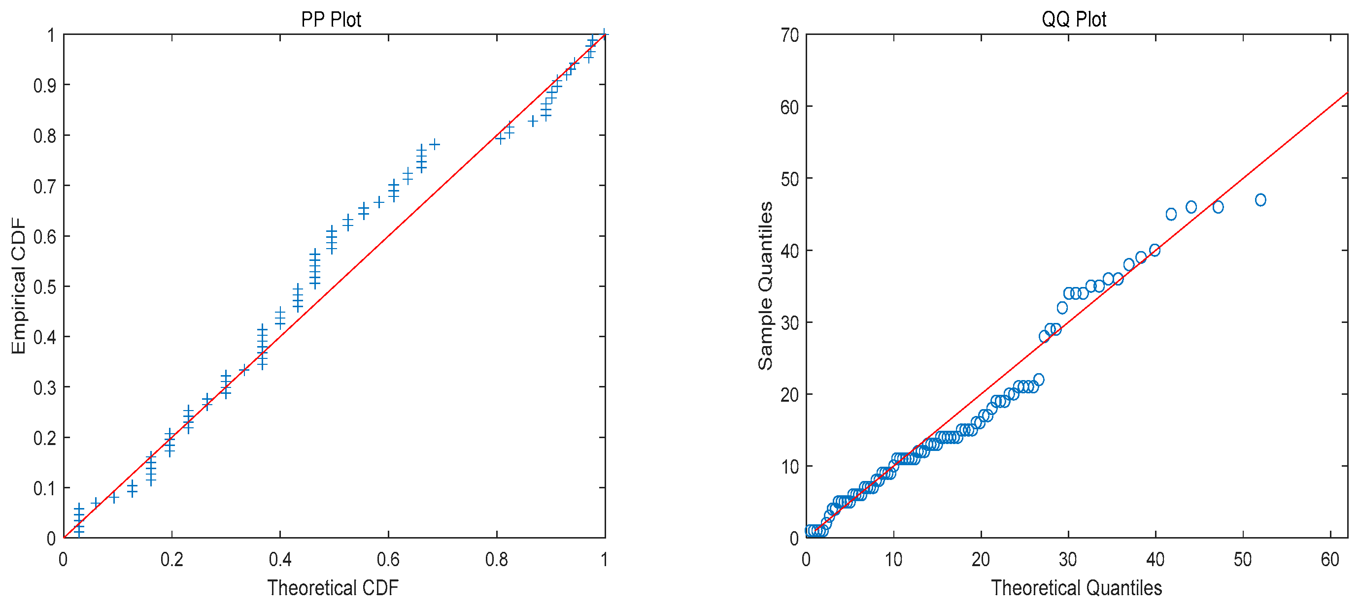
6. Analysis of Real Data
7. Conclusions
Author Contributions
Funding
Data Availability Statement
Conflicts of Interest
References
- Seong, K.; Lee, K. Exact likelihood inference for parameter of Exponential distribution under combined Generalized progressive hybrid censoring scheme. Symmetry 2022, 14, 1764. [Google Scholar] [CrossRef]
- Ateya, S.F.; Kilai, M.; Aldallal, R. Estimation using suggested EM algorithm based on progressively Type-II censored samples from a finite mixture of truncated Type-I generalized logistic distributions with an application. Math. Probl. Eng. 2022, 2022, 1720033. [Google Scholar] [CrossRef]
- Alotaibi, R.; Nassar, M.; Elshahhat, A. Estimations of modified Lindley parameters using progressive Type-II censoring with applications. Axioms 2023, 12, 171. [Google Scholar] [CrossRef]
- Balasooriya, U. Failure-censored reliability sampling plans for the exponential distribution. J. Stat. Comput. Simul. 1995, 52, 337–349. [Google Scholar] [CrossRef]
- Dykstra, O. Theory and technique of variation research. Technometrics 1964, 7, 654–655. [Google Scholar] [CrossRef]
- Wu, S.J.; Kuş, C. On estimation based on progressive first-failure censored sampling. Comput. Stat. Data Anal. 2009, 53, 3659–3670. [Google Scholar] [CrossRef]
- Shi, X.L.; Shi, Y.M. Estimation of stress-strength reliability for beta log Weibull distribution using progressive first-failure censored samples. Qual. Reliab. Eng. Int. 2023, 39, 1352–1375. [Google Scholar] [CrossRef]
- Abu-Moussa, M.H.; Alsadat, N.; Sharawy, A. On estimation of reliability functions for the extended Rayleigh distribution under progressive first-failure censoring model. Axioms 2023, 12, 680. [Google Scholar] [CrossRef]
- Elshahhat, A.; Sharma, V.K.; Mohammed, H.S. Statistical analysis of progressively first-failure censored data via beta-binomial removals. Aims Math. 2023, 8, 22419–22446. [Google Scholar] [CrossRef]
- Eliwa, M.S.; Ahmed, E.A. Reliability analysis of constant partially accelerated life tests under progressive first-failure Type-II censored data from Lomax model: EM and MCMC algorithms. Aims Math. 2023, 8, 29–60. [Google Scholar] [CrossRef]
- Surles, J.G.; Padgett, W.J. Inference for reliability and stress-strength for a scaled Burr type X distribution. Lifetime Data Anal. 2001, 7, 187–200. [Google Scholar] [CrossRef]
- Shen, Z.J.; Alrumayh, A.; Ahmad, Z.; Shanab, R.A.; Mutairi, M.A.; Aldallal, R. A new generalized Rayleigh distribution with analysis to big data of an online community. Alex. Eng. J. 2022, 61, 11523–11535. [Google Scholar] [CrossRef]
- Rabie, A.; Hussam, E.; Muse, A.H.; Aldallal, R.A.; Alharthi, A.S.; Aljohani, H.M. Estimations in a constant-stress partially accelerated life test for generalized Rayleigh distribution under Type-II hybrid censoring scheme. J. Mathem. 2022, 2022, 6307435. [Google Scholar] [CrossRef]
- Ren, J.; Gui, W.H. Inference and optimal censoring scheme for progressively Type-II censored competing risks model for generalized Rayleigh distribution. Comput. Stat. 2021, 36, 479–513. [Google Scholar] [CrossRef]
- Yang, L.Z.; Tsang, E.C.C.; Wang, X.Z.; Zhang, C.L. ELM parameter estimation in view of maximum likelihood. Neurocomputing 2023, 557, 126704. [Google Scholar] [CrossRef]
- Liu, Y.; Liu, B.D. Estimating unknown parameters in uncertain differential equation by maximum likelihood estimation. Soft. Comput. 2022, 26, 2773–2780. [Google Scholar] [CrossRef]
- Rasekhi, M.; Saber, M.M.; Hamedani, G.G.; El-Raouf, M.M.A.; Aldallal, R.; Gemeay, A.M. Approximate maximum likelihood estimations for the parameters of the generalized gudermannian distribution and its characterizations. J. Math. 2022, 2022, 2314–4629. [Google Scholar] [CrossRef]
- Cai, Y.X.; Gui, W.H. Classical and Bayesian inference for a progressive first-failure censored left-truncated normal distribution. Symmetry 2021, 13, 490. [Google Scholar] [CrossRef]
- Ng, H.K.T.; Chan, P.S.; Balakrishnan, N. Estimation of parameters from progressively censored data using EM algorithm. Comput. Stat. Data 2002, 39, 371–386. [Google Scholar] [CrossRef]
- Cho, H.; Kirch, C. Bootstrap confidence intervals for multiple change points based on moving sum procedures. Comput. Stat. Data Anal. 2022, 175, 107552. [Google Scholar] [CrossRef]
- Saegusa, T.; Sugasawa, S.; Lahiri, P. Parametric bootstrap confidence intervals for the multivariate Fay–Herriot model. J. Surv. Stat. Methodol. 2022, 10, 115–130. [Google Scholar] [CrossRef]
- Sroka, L. Comparison of jackknife and bootstrap methods in estimating confidence intervals. Sci. Pap. Silesian Univ. Technol. Organ. Manag. Ser. 2021, 153, 445–455. [Google Scholar] [CrossRef]
- Song, X.F.; Xiong, Z.Y.; Gui, W.H. Parameter estimation of exponentiated half-logistic distribution for left-truncated and right-censored data. Mathematics 2022, 10, 3838. [Google Scholar] [CrossRef]
- Han, M. Take a look at the hierarchical Bayesian estimation of parameters from several different angles. Commun. Stat. Theory Methods 2022, 52, 7718–7730. [Google Scholar] [CrossRef]
- Tiago, S.; Florian, L.; Denis, H. Bayesian estimation of decay parameters in Hawkes processes. Intell. Data Anal. 2023, 27, 223–240. [Google Scholar]
- Bangsgaard, K.O.; Andersen, M.; Heaf, J.G.; Ottesen, J.T. Bayesian parameter estimation for phosphate dynamics during hemodialysis. Math. Biosci. Eng. 2023, 20, 4455–4492. [Google Scholar] [CrossRef] [PubMed]
- Vaglio, M.; Pacilio, C.; Maselli, A.; Pani, P. Bayesian parameter estimation on boson-star binary signals with a coherent inspiral template and spin-dependent quadrupolar corrections. Phys. Rev. D 2023, 108, 023021. [Google Scholar] [CrossRef]
- Renjini, K.R.; Sathar, E.I.A.; Rajesh, G. A study of the effect of loss functions on the Bayes estimates of dynamic cumulative residual entropy for Pareto distribution under upper record values. J. Stat. Comput. Simul. 2016, 86, 324–339. [Google Scholar] [CrossRef]
- Sadoun, A.; Zeghdoudi, H.; Attoui, F.Z.; Remita, M.R. On Bayesian premium estimators for gamma lindley model under squared error loss function and linex loss function. J. Math. Stat. 2017, 13, 284–291. [Google Scholar] [CrossRef]
- Malgorzata, M. Bayesian estimation for non zero inflated modified power series distribution under linex and generalized entropy loss functions. Commun. Stat. Theory Methods 2016, 45, 3952–3969. [Google Scholar]
- Wasan, M.T. Parametric Estimation; McGraw-Hill Book Company: New York, NY, USA, 1970. [Google Scholar]
- Norstrom, J.G. The use of precautionary loss functions in risk analysis. IEEE Trans. Reliab. Theory 1996, 45, 400–403. [Google Scholar] [CrossRef]
- Han, M. A note on the posterior risk of the entropy loss function. Appl. Math. Model. 2023, 117, 705–713. [Google Scholar] [CrossRef]
- Abdel-Aty, Y.; Kayid, M.; Alomani, G. Generalized Bayes estimation based on a joint Type-II censored sample from K-exponential populations. Mathematics 2023, 11, 2190. [Google Scholar] [CrossRef]
- Ren, H.P.; Gong, Q.; Hu, X. Estimation of entropy for generalized Rayleigh distribution under progressively Type-II censored samples. Axioms 2023, 12, 776. [Google Scholar] [CrossRef]
- Han, M. E-Bayesian estimations of parameter and its evaluation standard: E-MSE (expected mean square error) under different loss functions. Commun. Stat. Simul. Comput. 2021, 50, 1971–1988. [Google Scholar] [CrossRef]
- Ali, S.; Aslam, M.; Kazmi, S.M.A. A study of the effect of the loss function on Bayes estimate, posterior risk and hazard function for lindley distribution. Appl. Math. Model. 2013, 37, 6068–6078. [Google Scholar] [CrossRef]
- Wei, Z.D. Parameter estimation of buffer autoregressive models based on Bayesian inference. Stat. Appl. 2023, 12, 32–39. [Google Scholar]
- Zhao, S.Y. Parameter estimation of logistic regression model based on MCMC algorithm—A case study of smart sleep bracelet. Mod. Comput. 2022, 28, 57–61. [Google Scholar]
- Asar, Y.; Belaghi, R.A. Estimation in Weibull distribution under progressively Type-I hybrid censored data. REVSTAT-Stat. J. 2023, 20, 563–586. [Google Scholar]
- Yang, K.; Zhang, Q.Q.; Yu, X.Y.; Dong, X.G. Bayesian inference for a mixture double autoregressive model. Stat. Neerlandica 2023, 77, 188–207. [Google Scholar] [CrossRef]
- Chen, X.Y.; Wang, J.J.; Yang, S.J. Semi-parametric hierarchical Bayesian modeling and optimization. Syst. Eng. Electron. 2023, 45, 1580–1588. [Google Scholar]
- Wang, X.Y.; Gui, W.H. Bayesian estimation of entropy for burr type XII distribution under progressive Type-II censored data. Mathematics 2021, 9, 313. [Google Scholar] [CrossRef]
- Balakrishnan, N.; Sandhu, R.A. A simple simulational algorithm for generating progressive Type-II censored samples. Am. Stat. 1995, 49, 229–230. [Google Scholar] [CrossRef]
- Bjerkedal, T. Acquisition of resistance in guinea pigs infected with different doses of virulent tubercle bacilli. Am. J. Epidemiol. 1960, 72, 130–148. [Google Scholar] [CrossRef] [PubMed]
- Alshunnar, F.S.; Raqab, M.Z.; Kundu, D. On the comparison of the Fisher information of the log-normal and generalized Rayleigh distributions. J. Appl. Stat. 2010, 37, 391–404. [Google Scholar] [CrossRef]
- Alahmadi, A.A.; Alqawba, M.; Almutiry, W.; Shawki, A.W.; Alrajhi, S.; Al-Marzouki, S.; Elgarhy, M. A New version of Weighte Weibull distribution: Modelling to COVID-19 data. Discret. Dyn. Nat. Soc. 2022, 2022, 3994361. [Google Scholar] [CrossRef]

| Algorithm: | Constructing Boot-t CI. |
|---|---|
| Step 1: | Setting the number of simulations B. |
| Step 2: | Obtaining the ML estimates and for parameters using the original censoring sample data . |
| Step 3: | Using the same censoring scheme, substitute the and obtained from step 2 into the CDF of the GRD to obtain a bootstrapped sample , and then obtain the bootstrapped ML estimates and and their variances and through the bootstrapped sample . |
| Step 4: | The statistical quantities and , as well as their CDFs and , are calculated from the bootstrap ML estimates and . |
| Step 5: | Repeated steps 3–4 for a total of B times, resulting in a series of Boot-t statistics and . |
| Step 6: | The obtained series of Boot-t statistics are sorted in ascending order to obtain and . |
| Loss Function | Bayes Estimator |
|---|---|
| SELF: | |
| GELF: | |
| WSELF: | |
| KLF: | |
| M/Q SELF: | |
| PLF: |
| Loss Function | Bayesian Estimator | ||
|---|---|---|---|
| Parameters | RF | HF | |
| SELF | |||
| GELF | |||
| WSELF | |||
| KLF | |||
| M/Q SELF | |||
| PLF | |||
| Scheme | |
|---|---|
| a | |
| b | |
| c |
| k | (n, m) | Q | NR | EM | k | (n, m) | Q | NR | EM | ||||||
|---|---|---|---|---|---|---|---|---|---|---|---|---|---|---|---|
| 2 | (30, 20) | a | 0.8842 | (0.0651) | 0.9722 | (0.0313) | r(t = 0.8) | 2 | (30, 20) | a | 0.4252 | (0.0107) | 0.3691 | (0.0164) | |
| b | 0.8928 | (0.0586) | 1.6036 | (0.6622) | b | 0.4216 | (0.0102) | 0.5000 | (0.0205) | ||||||
| c | 0.8663 | (0.0447) | 0.9553 | (0.0274) | c | 0.4308 | (0.0083) | 0.3780 | (0.0167) | ||||||
| (50, 30) | a | 0.8579 | (0.0382) | 0.9730 | (0.0308) | (50, 30) | a | 0.4334 | (0.0064) | 0.3596 | (0.0155) | ||||
| b | 0.8527 | (0.0294) | 1.8086 | (1.0321) | b | 0.4308 | (0.0069) | 0.5422 | (0.0229) | ||||||
| c | 0.8487 | (0.0309) | 0.9583 | (0.0270) | c | 0.4385 | (0.0050) | 0.3768 | (0.0141) | ||||||
| (80, 50) | a | 0.8423 | (0.0205) | 0.9710 | (0.0298) | (80, 50) | a | 0.4233 | (0.0037) | 0.3681 | (0.0112) | ||||
| b | 0.8262 | (0.0128) | 1.7139 | (0.8430) | b | 0.4398 | (0.0038) | 0.5304 | (0.0145) | ||||||
| c | 0.8291 | (0.0154) | 0.9543 | (0.0251) | c | 0.4412 | (0.0030) | 0.3791 | (0.0105) | ||||||
| 3 | (30, 20) | a | 0.9032 | (0.0630) | 0.9838 | (0.0344) | 3 | (30, 20) | a | 0.4102 | (0.0139) | 0.3451 | (0.0215) | ||
| b | 0.8763 | (0.0531) | 1.5236 | (0.5272) | b | 0.4144 | (0.0135) | 0.5511 | (0.0258) | ||||||
| c | 0.8607 | (0.0444) | 0.9715 | (0.0307) | c | 0.4264 | (0.0088) | 0.3554 | (0.0211) | ||||||
| (50, 30) | a | 0.8586 | (0.0327) | 0.9847 | (0.0344) | (50, 30) | a | 0.4208 | (0.0103) | 0.3351 | (0.0199) | ||||
| b | 0.8432 | (0.0237) | 1.6931 | (0.8001) | b | 0.4258 | (0.0081) | 0.6029 | (0.0338) | ||||||
| c | 0.8450 | (0.0246) | 0.9722 | (0.0303) | c | 0.4340 | (0.0060) | 0.3530 | (0.0172) | ||||||
| (80, 50) | a | 0.8343 | (0.0158) | 0.9829 | (0.0336) | (80, 50) | a | 0.4320 | (0.0058) | 0.3394 | (0.0166) | ||||
| b | 0.8830 | (0.0142) | 1.6227 | (0.6784) | b | 0.4348 | (0.0052) | 0.5918 | (0.0261) | ||||||
| c | 0.8273 | (0.0134) | 0.9703 | (0.0295) | c | 0.4380 | (0.0048) | 0.3529 | (0.0147) | ||||||
| 2 | (30, 20) | a | 1.0964 | (0.0808) | 1.2473 | (0.0909) | h(t = 0.8) | 2 | (30, 20) | a | 2.1290 | (1.0525) | 2.5528 | (1.1951) | |
| b | 1.0965 | (0.0717) | 1.2863 | (0.1169) | b | 2.1370 | (0.9762) | 2.3645 | (1.1512) | ||||||
| c | 1.0634 | (0.0451) | 1.2245 | (0.0823) | c | 1.9231 | (0.4184) | 2.4764 | (1.1039) | ||||||
| (50, 30) | a | 1.0595 | (0.0496) | 1.2605 | (0.0897) | (50, 30) | a | 1.9924 | (0.5380) | 2.5931 | (1.1116) | ||||
| b | 1.0701 | (0.0408) | 1.2821 | (0.1043) | b | 1.9558 | (0.4125) | 2.2209 | (0.7645) | ||||||
| c | 1.0472 | (0.0265) | 1.2248 | (0.0745) | c | 1.8726 | (0.2336) | 2.4634 | (0.9240) | ||||||
| (80, 50) | a | 1.0347 | (0.0264) | 1.2405 | (0.0702) | (80, 50) | a | 1.8656 | (0.2287) | 2.4997 | (0.7864) | ||||
| b | 1.0242 | (0.0202) | 1.2710 | (0.0868) | b | 1.8681 | (0.2692) | 2.2012 | (0.4902) | ||||||
| c | 1.0209 | (0.0142) | 1.2142 | (0.0600) | c | 1.8050 | (0.1167) | 2.4096 | (0.6838) | ||||||
| 3 | (30, 20) | a | 1.1031 | (0.0941) | 1.2982 | (0.1245) | 3 | (30, 20) | a | 2.2133 | (1.3141) | 2.7623 | (1.7360) | ||
| b | 1.1070 | (0.0926) | 1.1858 | (0.0659) | b | 2.1488 | (1.1277) | 1.9918 | (0.6252) | ||||||
| c | 1.0673 | (0.0472) | 1.2762 | (0.1162) | c | 1.9823 | (0.5537) | 2.6855 | (1.6634) | ||||||
| (50, 30) | a | 1.0775 | (0.0598) | 1.3101 | (0.1181) | (50, 30) | a | 2.0362 | (0.7900) | 2.7898 | (1.5223) | ||||
| b | 1.0662 | (0.0518) | 1.1632 | (0.0463) | b | 1.9644 | (0.5173) | 1.7905 | (0.3320) | ||||||
| c | 1.0530 | (0.0329) | 1.2729 | (0.0979) | c | 1.9191 | (0.3502) | 2.6459 | (1.2474) | ||||||
| (80, 50) | a | 1.0459 | (0.0349) | 1.2973 | (0.1018) | (80, 50) | a | 1.9041 | (0.3268) | 2.7242 | (1.2120) | ||||
| b | 1.0404 | (0.0262) | 1.1571 | (0.0358) | b | 1.8764 | (0.2589) | 1.7889 | (0.1754) | ||||||
| c | 1.0285 | (0.0169) | 1.2680 | (0.0868) | c | 1.8497 | (0.1807) | 2.6141 | (1.0279) | ||||||
| k | (n, m) | Q | Inf | Non-Inf | ||||||||||
|---|---|---|---|---|---|---|---|---|---|---|---|---|---|---|
| BS | BG | BW | BK | BM | BP | BS | BG | BW | BK | BM | BP | |||
| 2 | (30, 20) | a | 0.6933 (0.0114) | 0.6635 (0.0186) | 0.6540 (0.0213) | 0.6733 (0.0160) | 0.6179 (0.0331) | 0.7140 (0.0074) | 0.6435 (0.0245) | 0.6219 (0.0317) | 0.6144 (0.0344) | 0.6288 (0.0293) | 0.5847 (0.0464) | 0.6572 (0.0204) |
| b | 0.6435 (0.0245) | 0.6307 (0.0287) | 0.6265 (0.0301) | 0.6349 (0.0272) | 0.6097 (0.0362) | 0.6522 (0.0218) | 0.6344 (0.0274) | 0.6157 (0.0340) | 0.6095 (0.0363) | 0.6218 (0.0317) | 0.5853 (0.0461) | 0.6470 (0.0234) | ||
| c | 0.6672 (0.0176) | 0.6420 (0.0250) | 0.6340 (0.0276) | 0.6504 (0.0224) | 0.6032 (0.0387) | 0.6848 (0.0133) | 0.6390 (0.0259) | 0.6182 (0.0331) | 0.6114 (0.0356) | 0.6251 (0.0306) | 0.5849 (0.0463) | 0.6532 (0.0215) | ||
| (50, 30) | a | 0.7184 (0.0067) | 0.6977 (0.0105) | 0.6911 (0.0118) | 0.7074 (0.0091) | 0.6660 (0.0180) | 0.7328 (0.0045) | 0.6476 (0.0232) | 0.6282 (0.0295) | 0.6215 (0.0319) | 0.6344 (0.0274) | 0.5944 (0.0423) | 0.6599 (0.0196) | |
| b | 0.6816 (0.0140) | 0.6704 (0.0168) | 0.6668 (0.0178) | 0.6741 (0.0158) | 0.6526 (0.0217) | 0.6893 (0.0123) | 0.6793 (0.0146) | 0.6643 (0.0184) | 0.6590 (0.0199) | 0.6691 (0.0171) | 0.6370 (0.0266) | 0.6888 (0.0124) | ||
| c | 0.7472 (0.0028) | 0.7288 (0.0051) | 0.7225 (0.0060) | 0.7347 (0.0043) | 0.6970 (0.0106) | 0.7593 (0.0017) | 0.7158 (0.0071) | 0.6952 (0.0110) | 0.6885 (0.0124) | 0.7020 (0.0096) | 0.6622 (0.0190) | 0.7298 (0.0049) | ||
| (80, 50) | a | 0.7445 (0.0031) | 0.7306 (0.0048) | 0.7260 (0.0055) | 0.7352 (0.0042) | 0.7078 (0.0085) | 0.7538 (0.0021) | 0.7215 (0.0062) | 0.7102 (0.0081) | 0.7064 (0.0088) | 0.7139 (0.0074) | 0.6914 (0.0118) | 0.7290 (0.0050) | |
| b | 0.7206 (0.0063) | 0.7113 (0.0079) | 0.7083 (0.0084) | 0.7144 (0.0073) | 0.6964 (0.0107) | 0.7269 (0.0053) | 0.6972 (0.0106) | 0.6884 (0.0125) | 0.6855 (0.0131) | 0.6914 (0.0118) | 0.6744 (0.0158) | 0.7033 (0.0093) | ||
| c | 0.7583 (0.0017) | 0.7440 (0.0031) | 0.7393 (0.0037) | 0.7487 (0.0026) | 0.7205 (0.0063) | 0.7680 (0.0010) | 0.7361 (0.0041) | 0.7261 (0.0055) | 0.7227 (0.0060) | 0.7294 (0.0050) | 0.7092 (0.0082) | 0.7427 (0.0033) | ||
| 3 | (30, 20) | a | 0.6917 (0.0117) | 0.6626 (0.0189) | 0.6530 (0.0216) | 0.6721 (0.0164) | 0.6155 (0.0341) | 0.7113 (0.0079) | 0.6709 (0.0167) | 0.6468 (0.0235) | 0.6392 (0.0258) | 0.6549 (0.0211) | 0.6106 (0.0359) | 0.6883 (0.0125) |
| b | 0.6586 (0.0200) | 0.6437 (0.0244) | 0.6389 (0.0260) | 0.6487 (0.0229) | 0.6200 (0.0324) | 0.6688 (0.0172) | 0.6167 (0.0336) | 0.5976 (0.0410) | 0.5914 (0.0435) | 0.6039 (0.0384) | 0.5673 (0.0541) | 0.6297 (0.0290) | ||
| c | 0.6713 (0.0166) | 0.6526 (0.0217) | 0.6461 (0.0237) | 0.6585 (0.0200) | 0.6189 (0.0328 | 0.6830 (0.0137) | 0.6359 (0.0269) | 0.6169 (0.0335) | 0.6105 (0.0359) | 0.6231 (0.0313) | 0.5845 (0.0464) | 0.6484 (0.0230 | ||
| (50, 30) | a | 0.7162 (0.0070) | 0.6998 (0.0100) | 0.6943 (0.0112) | 0.7052 (0.0090) | 0.6730 (0.0161) | 0.7274 (0.0053) | 0.6567 (0.0206) | 0.6354 (0.0271) | 0.6281 (0.0296) | 0.6422 (0.0249) | 0.5986 (0.0406) | 0.6700 (0.0169) | |
| b | 0.6942 (0.0112) | 0.6819 (0.0139) | 0.6778 (0.0149) | 0.6860 (0.0130) | 0.6618 (0.0191) | 0.7024 (0.0095) | 0.6892 (0.0123) | 0.6744 (0.0158) | 0.6695 (0.0170) | 0.6793 (0.0146) | 0.6500 (0.0225) | 0.6991 (0.0102) | ||
| c | 0.7397 (0.0036) | 0.7236 (0.0058) | 0.7182 (0.0067) | 0.7288 (0.0051) | 0.6964 (0.0107) | 0.7503 (0.0025) | 0.7280 (0.0052) | 0.7115 (0.0078) | 0.7059 (0.0088) | 0.7169 (0.0069) | 0.6839 (0.0135) | 0.7389 (0.0037) | ||
| (80, 50) | a | 0.7388 (0.0037) | 0.7273 (0.0053) | 0.7235 (0.0059) | 0.7311 (0.0048) | 0.7082 (0.0084) | 0.7465 (0.0029) | 0.7197 (0.0065) | 0.7094 (0.0082) | 0.7059 (0.0089) | 0.7127 (0.0076) | 0.6911 (0.0119) | 0.7261 (0.0055) | |
| b | 0.7107 (0.0080) | 0.7046 (0.0091) | 0.7026 (0.0095) | 0.7066 (0.0087) | 0.6942 (0.0112) | 0.7146 (0.0073) | 0.6857 (0.0131) | 0.6788 (0.0147) | 0.6765 (0.0152) | 0.6811 (0.0141) | 0.6674 (0.0176) | 0.6903 (0.0120) | ||
| c | 0.7586 (0.0017) | 0.7490 (0.0026) | 0.7460 (0.0029) | 0.7523 (0.0023) | 0.7341 (0.0043) | 0.7653 (0.0012) | 0.7366 (0.0040) | 0.7275 (0.0053) | 0.7244 (0.0057) | 0.7305 (0.0048) | 0.7120 (0.0077) | 0.7426 (0.0033) | ||
| k | (n, m) | Q | Inf | Non-Inf | ||||||||||
|---|---|---|---|---|---|---|---|---|---|---|---|---|---|---|
| BS | BG | BW | BK | BM | BP | BS | BG | BW | BK | BM | BP | |||
| 2 | (30, 20) | a | 0.8360 (0.0269) | 0.8049 (0.0381) | 0.7936 (0.0426) | 0.8145 (0.0344) | 0.7456 (0.0647) | 0.8547 (0.0211) | 0.7498 (0.0626) | 0.7019 (0.0889) | 0.6860 (0.0986) | 0.7172 (0.0800) | 0.6251 (0.1406) | 0.7813 (0.0478) |
| b | 0.8910 (0.0119) | 0.8718 (0.0164) | 0.8651 (0.0182) | 0.8779 (0.0149) | 0.8370 (0.0266) | 0.9029 (0.0094) | 0.8739 (0.0159) | 0.8467 (0.0235) | 0.8376 (0.0264) | 0.8556 (0.0209) | 0.8014 (0.0395) | 0.8919 (0.0117) | ||
| c | 0.8976 (0.0105) | 0.8714 (0.0165) | 0.8622 (0.0190) | 0.8797 (0.0145) | 0.8242 (0.0309) | 0.9138 (0.0074) | 0.8707 (0.0167) | 0.8494 (0.0227) | 0.8419 (0.0250) | 0.8562 (0.0201) | 0.8112 (0.0357) | 0.8841 (0.0134) | ||
| (50, 30) | a | 0.8946 (0.0111) | 0.8665 (0.0178) | 0.8565 (0.0206) | 0.8753 (0.0155) | 0.8147 (0.0343) | 0.9118 (0.0078) | 0.8647 (0.0183) | 0.8459 (0.0238) | 0.8394 (0.0258) | 0.8520 (0.0219) | 0.8130 (0.0350) | 0.8767 (0.0152) | |
| b | 0.9215 (0.0062) | 0.8981 (0.0104) | 0.8898 (0.0121) | 0.9056 (0.0089) | 0.8556 (0.0209) | 0.9361 (0.0041) | 0.9197 (0.0064) | 0.8957 (0.0109) | 0.8875 (0.0127) | 0.9034 (0.0093) | 0.8542 (0.0213) | 0.9351 (0.0042) | ||
| c | 0.9401 (0.0036) | 0.9247 (0.0057) | 0.9194 (0.0065) | 0.9297 (0.0049) | 0.8977 (0.0105) | 0.9499 (0.0025) | 0.9150 (0.0072) | 0.9001 (0.0100) | 0.8952 (0.0110) | 0.9050 (0.0090) | 0.8756 (0.0155) | 0.9248 (0.0057) | ||
| (80, 50) | a | 0.9239 (0.0058) | 0.9086 (0.0083) | 0.9033 (0.0093) | 0.9136 (0.0075) | 0.8817 (0.0140) | 0.9336 (0.0044) | 0.9044 (0.0091) | 0.8885 (0.0124) | 0.8827 (0.0138) | 0.8935 (0.0113) | 0.8581 (0.0201) | 0.9142 (0.0074) | |
| b | 0.9445 (0.0031) | 0.9318 (0.0047) | 0.9274 (0.0053) | 0.9360 (0.0041) | 0.9101 (0.0081) | 0.9529 (0.0022) | 0.9328 (0.0045) | 0.9139 (0.0074) | 0.9073 (0.0086) | 0.9200 (0.0064) | 0.8799 (0.0144) | 0.9448 (0.0030) | ||
| c | 0.9676 (0.0011) | 0.9588 (0.0017) | 0.9557 (0.0020) | 0.9616 (0.0015) | 0.9435 (0.0032) | 0.9732 (0.0007) | 0.9572 (0.0018) | 0.9462 (0.0029) | 0.9424 (0.0033) | 0.9498 (0.0025) | 0.9269 (0.0053) | 0.9642 (0.0013) | ||
| 3 | (30, 20) | a | 0.8748 (0.0157) | 0.8371 (0.0265) | 0.8235 (0.0311) | 0.8488 (0.0229) | 0.7673 (0.0541) | 0.8973 (0.0105) | 0.7962 (0.0415) | 0.7328 (0.0714) | 0.7092 (0.0846) | 0.7515 (0.0618) | 0.6130 (0.1498) | 0.8322 (0.0282) |
| b | 0.8870 (0.0128) | 0.8544 (0.0212) | 0.8427 (0.0248) | 0.8645 (0.0184) | 0.7938 (0.0425) | 0.9066 (0.0087) | 0.8829 (0.0137) | 0.8378 (0.0263) | 0.8202 (0.0323) | 0.8510 (0.0222) | 0.7409 (0.0671) | 0.9084 (0.0084) | ||
| c | 0.9227 (0.0060) | 0.8987 (0.0103) | 0.8904 (0.0120) | 0.9064 (0.0088) | 0.8565 (0.0206) | 0.9380 (0.0038) | 0.8914 (0.0118) | 0.8593 (0.0198) | 0.8473 (0.0233) | 0.8691 (0.0171) | 0.7950 (0.0420) | 0.9103 (0.0080) | ||
| (50, 30) | a | 0.8905 (0.0120) | 0.8650 (0.0182) | 0.8562 (0.0207) | 0.8732 (0.0161) | 0.8205 (0.0322) | 0.9069 (0.0087) | 0.8344 (0.0274) | 0.8001 (0.0400) | 0.7879 (0.0450) | 0.8108 (0.0358) | 0.7382 (0.0686) | 0.8552 (0.0210) | |
| b | 0.9197 (0.0064) | 0.8864 (0.0129) | 0.8743 (0.0158) | 0.8967 (0.0107) | 0.8240 (0.0310) | 0.9398 (0.0036) | 0.8966 (0.0107) | 0.8655 (0.0181) | 0.8548 (0.0211) | 0.8755 (0.0155) | 0.8116 (0.0355) | 0.9168 (0.0069) | ||
| c | 0.9333 (0.0044) | 0.9173 (0.0068) | 0.9117 (0.0078) | 0.9225 (0.0060) | 0.8890 (0.0123) | 0.9433 (0.0032) | 0.9165 (0.0070) | 0.8965 (0.0107) | 0.8894 (0.0122) | 0.9029 (0.0094) | 0.8604 (0.0195) | 0.9289 (0.0051) | ||
| (80, 50) | a | 0.9084 (0.0084) | 0.8928 (0.0115) | 0.8874 (0.0127) | 0.8979 (0.0104) | 0.8659 (0.0180) | 0.9185 (0.0066) | 0.8856 (0.0131) | 0.8633 (0.0187) | 0.8553 (0.0209) | 0.8703 (0.0168) | 0.8221 (0.0317) | 0.8992 (0.0102) | |
| b | 0.9623 (0.0014) | 0.9461 (0.0029) | 0.9405 (0.0035) | 0.9513 (0.0024) | 0.9176 (0.0068) | 0.9728 (0.0007) | 0.9489 (0.0026) | 0.9253 (0.0056) | 0.9170 (0.0069) | 0.9328 (0.0045) | 0.8834 (0.0136) | 0.9639 (0.0013) | ||
| c | 0.9642 (0.0013) | 0.9530 (0.0022) | 0.9494 (0.0026) | 0.9567 (0.0019) | 0.9349 (0.0042) | 0.9716 (0.0008) | 0.9358 (0.0041) | 0.9261 (0.0055) | 0.9228 (0.0060) | 0.9293 (0.0050) | 0.9099 (0.0081) | 0.9423 (0.0033) | ||
| k | (n, m) | Q | Inf | Non-Inf | ||||||||||
|---|---|---|---|---|---|---|---|---|---|---|---|---|---|---|
| BS | BG | BW | BK | BM | BP | BS | BG | BW | BK | BM | BP | |||
| 2 | (30, 20) | a | 0.3743 (0.0059) | 0.3551 (0.0092) | 0.3481 (0.0106) | 0.3609 (0.0081) | 0.3186 (0.0175) | 0.3859 (0.0042) | 0.3474 (0.0107) | 0.3304 (0.0145) | 0.3245 (0.0160) | 0.3358 (0.0133) | 0.3011 (0.0224) | 0.3581 (0.0086) |
| b | 0.3963 (0.0030) | 0.3773 (0.0054) | 0.3705 (0.065) | 0.3831 (0.0046) | 0.3423 (0.0118) | 0.4078 (0.0019) | 0.3709 (0.0064) | 0.3501 (0.0102) | 0.3425 (0.0117) | 0.3564 (0.0089) | 0.3111 (0.0195) | 0.3833 (0.0046) | ||
| c | 0.3939 (0.0033) | 0.3815 (0.0048) | 0.3772 (0.0054) | 0.3854 (0.0043) | 0.3595 (0.0083) | 0.4017 (0.0024) | 0.3721 (0.0053) | 0.3599 (0.0083) | 0.3557 (0.0091) | 0.3638 (0.0076) | 0.3388 (0.0126) | 0.3862 (0.0051) | ||
| (50, 30) | a | 0.4078 (0.0019) | 0.3966 (0.0029) | 0.3927 (0.0034) | 0.4002 (0.0026) | 0.3763 (0.0056) | 0.4148 (0.0013) | 0.3824 (0.0047) | 0.3691 (0.0067) | 0.3645 (0.0075) | 0.3733 (0.0060) | 0.3458 (0.0110) | 0.3908 (0.0036) | |
| b | 0.4259 (0.0006) | 0.4164 (0.0012) | 0.4131 (0.0014) | 0.4195 (0.0010) | 0.3996 (0.0026) | 0.4320 (0.0004) | 0.3932 (0.0033) | 0.3808 (0.0049) | 0.3766 (0.0055) | 0.3848 (0.0044) | 0.3595 (0.0083) | 0.4012 (0.0025) | ||
| c | 0.3972 (0.0029) | 0.3863 (0.0042) | 0.3826 (0.0047) | 0.3898 (0.0037) | 0.3676 (0.0069) | 0.4042 (0.0022) | 0.3864 (0.0042) | 0.3765 (0.0055) | 0.3730 (0.0061) | 0.3796 (0.0051) | 0.3589 (0.0085) | 0.3926 (0.0034) | ||
| (80, 50) | a | 0.4233 (0.0008) | 0.4169 (0.0012) | 0.4147 (0.0013) | 0.4190 (0.0010) | 0.4057 (0.0020) | 0.4274 (0.0006) | 0.4127 (0.0015) | 0.4051 (0.0021) | 0.4025 (0.0023) | 0.4076 (0.0019) | 0.3918 (0.0035) | 0.4176 (0.0011) | |
| b | 0.4288 (0.0005) | 0.4228 (0.0008) | 0.4208 (0.0010) | 0.4248 (0.0007) | 0.4126 (0.0015) | 0.4326 (0.0003) | 0.4177 (0.0011) | 0.4101 (0.0017) | 0.4075 (0.0019) | 0.4126 (0.0015) | 0.3970 (0.0029) | 0.4226 (0.0008) | ||
| c | 0.4274 (0.0006) | 0.4227 (0.0008) | 0.4211 (0.0009) | 0.4243 (0.0007) | 0.4149 (0.0013) | 0.4305 (0.0004) | 0.4258 (0.0006) | 0.4214 (0.0009) | 0.4199 (0.0010) | 0.4228 (0.0008) | 0.4141 (0.0013) | 0.4287 (0.0005) | ||
| 3 | (30, 20) | a | 0.3833 (0.0046) | 0.3559 (0.0090) | 0.3448 (0.0112) | 0.3636 (0.0076) | 0.2918 (0.0258) | 0.3986 (0.0027) | 0.3514 (0.0099) | 0.3245 (0.0160) | 0.3157 (0.0183) | 0.3330 (0.0139) | 0.2823 (0.0284) | 0.3686 (0.0068) |
| b | 0.3902 (0.0037) | 0.3699 (0.0066) | 0.3624 (0.0078) | 0.3761 (0.0056) | 0.3301 (0.0146) | 0.4026 (0.0023) | 0.3734 (0.0060) | 0.3459 (0.0110) | 0.3356 (0.0133) | 0.3540 (0.0094) | 0.2901 (0.0259) | 0.3900 (0.0037) | ||
| c | 0.4012 (0.0025) | 0.3870 (0.0041) | 0.3820 (0.0047) | 0.3915 (0.0035) | 0.3619 (0.0079) | 0.4102 (0.0017) | 0.3815 (0.0048) | 0.3667 (0.0071) | 0.3616 (0.0080) | 0.3714 (0.0063) | 0.3407 (0.0121) | 0.3908 (0.0036) | ||
| (50, 30) | a | 0.4098 (0.0017) | 0.3976 (0.0028) | 0.3930 (0.0033) | 0.4013 (0.0025) | 0.3734 (0.0060) | 0.4172 (0.0011) | 0.3691 (0.0067) | 0.3430 (0.0116) | 0.3323 (0.0141) | 0.3502 (0.0101) | 0.2843 (0.0278) | 0.3829 (0.0046) | |
| b | 0.4182 (0.0011) | 0.4033 (0.0023) | 0.3983 (0.0028) | 0.4081 (0.0018) | 0.3783 (0.0053) | 0.4277 (0.0005) | 0.4174 (0.0011) | 0.3993 (0.0027) | 0.3924 (0.0034) | 0.4047 (0.0021) | 0.3624 (0.0078) | 0.4281 (0.0005) | ||
| c | 0.3954 (0.0031) | 0.3861 (0.0042) | 0.3830 (0.0046) | 0.3891 (0.0038) | 0.3702 (0.0065) | 0.4041 (0.0024) | 0.3933 (0.0033) | 0.3840 (0.0045) | 0.3808 (0.0049) | 0.3870 (0.0041) | 0.3681 (0.0068) | 0.3993 (0.0027) | ||
| (80, 50) | a | 0.4142 (0.0018) | 0.4017 (0.0024) | 0.3992 (0.0027) | 0.4040 (0.0022) | 0.3891 (0.0038) | 0.4136 (0.0014) | 0.3941 (0.0032) | 0.3856 (0.0043) | 0.3954 (0.0031) | 0.3883 (0.0039) | 0.3703 (0.0065) | 0.3995 (0.0026) | |
| b | 0.4248 (0.0007) | 0.4170 (0.0011) | 0.4144 (0.0013) | 0.4195 (0.0010) | 0.4035 (0.0022) | 0.4297 (0.0004) | 0.4111 (0.0016) | 0.4019 (0.0024) | 0.3987 (0.0027) | 0.4048 (0.0021) | 0.3857 (0.0042) | 0.4170 (0.0011) | ||
| c | 0.4387 (0.0001) | 0.4301 (0.0004) | 0.4272 (0.0006) | 0.4329 (0.0003) | 0.4155 (0.0013) | 0.4442 (0.0001) | 0.4370 (0.0002) | 0.4288 (0.0005) | 0.4259 (0.0006) | 0.4314 (0.0004) | 0.4138 (0.0014) | 0.4421 (0.0001) | ||
| k | (n, m) | Q | Inf | Non-Inf | ||||||||||
|---|---|---|---|---|---|---|---|---|---|---|---|---|---|---|
| BS | BG | BW | BK | BM | BP | BS | BG | BW | BK | BM | BP | |||
| 2 | (30, 20) | a | 1.5697 (0.0287) | 1.4251 (0.0985) | 1.3735 (0.1335) | 1.4683 (0.0732) | 1.1667 (0.3274) | 1.6569 (0.0067) | 1.4900 (0.0620) | 1.3755 (0.1321) | 1.3344 (0.1637) | 1.4100 (0.1082) | 1.1644 (0.3302) | 1.5605 (0.0318) |
| b | 1.5267 (0.0450) | 1.3825 (0.1271) | 1.3335 (0.1644) | 1.4268 (0.0974) | 1.1460 (0.3516) | 1.6181 (0.0146) | 1.4169 (0.0599) | 1.3715 (0.1350) | 1.3292 (0.1679) | 1.4086 (0.1091) | 1.1618 (0.3332) | 1.5684 (0.0291) | ||
| c | 1.5784 (0.0258) | 1.4882 (0.0629) | 1.4578 (0.0791) | 1.5169 (0.0493) | 1.3384 (0.1605) | 1.6377 (0.0103) | 1.5427 (0.0385) | 1.4402 (0.0893) | 1.4060 (0.1109) | 1.4728 (0.0709) | 1.2725 (0.2176) | 1.6105 (0.0165) | ||
| (50, 30) | a | 1.6180 (0.0146) | 1.5107 (0.0521) | 1.4754 (0.0694) | 1.5451 (0.0376) | 1.3420 (0.1576) | 1.6891 (0.0025) | 1.5582 (0.0327) | 1.4677 (0.0736) | 1.4381 (0.0905) | 1.4969 (0.0586) | 1.3257 (0.1708) | 1.6187 (0.0145) | |
| b | 1.6344 (0.0109) | 1.5479 (0.0365) | 1.5190 (0.0484) | 1.5756 (0.0267) | 1.4056 (0.1111) | 1.6910 (0.0023) | 1.5239 (0.0462) | 1.4260 (0.0980) | 1.3917 (0.1206) | 1.4563 (0.0799) | 1.2523 (0.2368) | 1.5861 (0.0234) | ||
| c | 1.6421 (0.0094) | 1.5804 (0.0251) | 1.5599 (0.0321) | 1.6005 (0.0192) | 1.4786 (0.0678) | 1.6834 (0.0031) | 1.5741 (0.0272) | 1.5117 (0.0517) | 1.4908 (0.0616) | 1.5319 (0.0429) | 1.4082 (0.1094) | 1.6156 (0.0152) | ||
| (80, 50) | a | 1.6718 (0.0045) | 1.5995 (0.0194) | 1.5764 (0.0264) | 1.6234 (0.0134) | 1.4894 (0.0623) | 1.7214 (0.0003) | 1.6345 (0.0109) | 1.5730 (0.0275) | 1.5532 (0.0345) | 1.5933 (0.0212) | 1.4769 (0.0687) | 1.6770 (0.0038) | |
| b | 1.6671 (0.0052) | 1.6145 (0.0155) | 1.5969 (0.0202) | 1.6317 (0.0115) | 1.5275 (0.0447) | 1.7018 (0.0014) | 1.6584 (0.0065) | 1.5973 (0.0201) | 1.5771 (0.0262) | 1.6172 (0.0148) | 1.4976 (0.0583) | 1.6991 (0.0016) | ||
| c | 1.6581 (0.0065) | 1.6143 (0.0155) | 1.5997 (0.0194) | 1.6286 (0.0122) | 1.5418 (0.0389) | 1.6872 (0.0027) | 1.5950 (0.0207) | 1.5535 (0.0344) | 1.5393 (0.0399) | 1.5669 (0.0296) | 1.4812 (0.0665) | 1.6216 (0.0138) | ||
| 3 | (30, 20) | a | 1.5573 (0.0330) | 1.3927 (0.1199) | 1.3334 (0.1645) | 1.4410 (0.0888) | 1.0984 (0.4103) | 1.6546 (0.0071) | 1.3598 (0.1438) | 1.1956 (0.2953) | 1.1409 (0.3577) | 1.2455 (0.2435) | 0.9412 (0.6364) | 1.4626 (0.0764) |
| b | 1.5614 (0.0315) | 1.4386 (0.0902) | 1.3969 (0.1170) | 1.4769 (0.0687) | 1.2352 (0.2538) | 1.6401 (0.0098) | 1.3753 (0.1323) | 1.2506 (0.2385) | 1.2074 (0.2825) | 1.2886 (0.2028) | 1.0380 (0.4913) | 1.4541 (0.0812) | ||
| c | 1.5846 (0.0238) | 1.4883 (0.0629) | 1.4559 (0.0801) | 1.5189 (0.0484) | 1.3293 (0.1678) | 1.6475 (0.0084) | 1.5575 (0.0329) | 1.4648 (0.0751) | 1.4343 (0.0928) | 1.4946 (0.0597) | 1.3163 (0.1787) | 1.6199 (0.0142) | ||
| (50, 30) | a | 1.6116 (0.0162) | 1.4895 (0.0622) | 1.4500 (0.0835) | 1.5287 (0.0442) | 1.2999 (0.1927) | 1.6954 (0.0019) | 1.5799 (0.0253) | 1.4518 (0.0825) | 1.4098 (0.1084) | 1.4924 (0.0608) | 1.2511 (0.2381) | 1.6639 (0.0056) | |
| b | 1.6188 (0.0144) | 1.5323 (0.0427) | 1.5030 (0.0557) | 1.5598 (0.0321) | 1.3861 (0.1245) | 1.6755 (0.0040) | 1.5347 (0.0417) | 1.4357 (0.0920) | 1.4029 (0.1129) | 1.4673 (0.0738) | 1.2766 (0.2138) | 1.6005 (0.0192) | ||
| c | 1.6196 (0.0143) | 1.5422 (0.0387) | 1.5168 (0.0494) | 1.5673 (0.0295) | 1.4183 (0.1028) | 1.6719 (0.0045) | 1.5809 (0.0250) | 1.5011 (0.0566) | 1.4750 (0.0697) | 1.5270 (0.0449) | 1.3737 (0.1334) | 1.6347 (0.0109) | ||
| (80, 50) | a | 1.6138 (0.0157) | 1.5474 (0.0367) | 1.5257 (0.0455) | 1.5692 (0.0288) | 1.4425 (0.0879) | 1.6585 (0.0065) | 1.5791 (0.0256) | 1.4785 (0.0679) | 1.4429 (0.0877) | 1.5095 (0.0527) | 1.3001 (0.1926) | 1.6404 (0.0097) | |
| b | 1.6443 (0.0090) | 1.5790 (0.0256) | 1.5575 (0.0329) | 1.6003 (0.0192) | 1.4731 (0.0707) | 1.6888 (0.0025) | 1.5847 (0.0238) | 1.5151 (0.0501) | 1.4926 (0.0607) | 1.5380 (0.0404) | 1.4059 (0.1109) | 1.6325 (0.0113) | ||
| c | 1.6469 (0.0085) | 1.5953 (0.0206) | 1.5779 (0.0260) | 1.6120 (0.0161) | 1.5147 (0.0503) | 1.6808 (0.0034) | 1.6254 (0.0129) | 1.5777 (0.0260) | 1.5618 (0.0314) | 1.5933 (0.0212) | 1.4991 (0.0575) | 1.6573 (0.0067) | ||
| k | (n, m) | Q | Boot-t CI | Inf | Non-Inf | k | (n, m) | Q | Boot-t CI | Inf | Non-Inf | ||
|---|---|---|---|---|---|---|---|---|---|---|---|---|---|
| Cred.CI | Cred.CI | Cres.CI | Cred.CI | ||||||||||
| AW | AW | AW | AW | AW | AW | ||||||||
| 2 | (30, 20) | a | 1.4408 | 0.3043 | 0.3493 | r(t = 0.8) | 2 | (30, 20) | a | 0.3748 | 0.2299 | 0.2558 | |
| b | 0.9306 | 0.2654 | 0.3087 | b | 0.3075 | 0.2473 | 0.2483 | ||||||
| c | 0.8049 | 0.3934 | 0.4093 | c | 0.6809 | 0.2190 | 0.2255 | ||||||
| (50, 30) | a | 0.8956 | 0.2961 | 0.3356 | (50, 30) | a | 0.3513 | 0.1792 | 0.1888 | ||||
| b | 0.5480 | 0.2617 | 0.2878 | b | 0.2898 | 0.1970 | 0.1984 | ||||||
| c | 0.6534 | 0.3598 | 0.3906 | c | 0.5727 | 0.2027 | 0.2070 | ||||||
| (80, 50) | a | 0.5675 | 0.2831 | 0.3187 | (80, 50) | a | 0.2898 | 0.1604 | 0.1787 | ||||
| b | 0.4079 | 0.2600 | 0.2784 | b | 0.2163 | 0.1405 | 0.1637 | ||||||
| c | 0.5974 | 0.2801 | 0.3004 | c | 0.4755 | 0.1350 | 0.1458 | ||||||
| 3 | (30, 20) | a | 1.3254 | 0.2947 | 0.3358 | 3 | (30, 20) | a | 0.2564 | 0.2040 | 0.2420 | ||
| b | 0.7471 | 0.2399 | 0.2849 | b | 0.3042 | 0.2383 | 0.2412 | ||||||
| c | 0.6702 | 0.3328 | 0.3849 | c | 0.5577 | 0.2029 | 0.2122 | ||||||
| (50, 30) | a | 0.5153 | 0.2805 | 0.3144 | (50, 30) | a | 0.2434 | 0.1662 | 0.1720 | ||||
| b | 0.4607 | 0.2032 | 0.2214 | b | 0.2338 | 0.1792 | 0.1950 | ||||||
| c | 0.5053 | 0.3289 | 0.3793 | c | 0.5368 | 0.1610 | 0.1710 | ||||||
| (80, 50) | a | 0.5001 | 0.2579 | 0.2602 | (80, 50) | a | 0.1571 | 0.1475 | 0.1646 | ||||
| b | 0.3713 | 0.1812 | 0.1842 | b | 0.1897 | 0.1284 | 0.1602 | ||||||
| c | 0.4971 | 0.2525 | 0.2832 | c | 0.4701 | 0.1329 | 0.1352 | ||||||
| 2 | (30, 20) | a | 1.5109 | 0.4861 | 0.5986 | h(t = 0.8) | 2 | (30, 20) | a | 2.4525 | 1.0215 | 1.0661 | |
| b | 1.3316 | 0.5701 | 0.6062 | b | 2.2799 | 1.5842 | 1.6715 | ||||||
| c | 1.8853 | 0.5502 | 0.5745 | c | 4.9014 | 1.2195 | 1.3793 | ||||||
| (50, 30) | a | 1.2356 | 0.4518 | 0.4859 | (50, 30) | a | 2.3585 | 0.8768 | 0.8962 | ||||
| b | 0.8538 | 0.4818 | 0.5276 | b | 1.8764 | 1.4697 | 1.6348 | ||||||
| c | 1.5827 | 0.3583 | 0.4638 | c | 4.5132 | 1.1207 | 1.2353 | ||||||
| (80, 50) | a | 1.0531 | 0.3619 | 0.4065 | (80, 50) | a | 2.2304 | 0.7948 | 0.8730 | ||||
| b | 0.7125 | 0.3229 | 0.3867 | b | 1.2160 | 0.9789 | 1.0538 | ||||||
| c | 0.9611 | 0.3064 | 0.3269 | c | 3.9968 | 0.7289 | 0.9098 | ||||||
| 3 | (30, 20) | a | 1.4238 | 0.4458 | 0.5213 | 3 | (30, 20) | a | 2.3612 | 1.0046 | 1.0216 | ||
| b | 1.1445 | 0.5046 | 0.5901 | b | 2.2455 | 1.2139 | 1.3956 | ||||||
| c | 1.3713 | 0.4295 | 0.4746 | c | 4.2802 | 1.1100 | 1.3018 | ||||||
| (50, 30) | a | 1.1092 | 0.4240 | 0.4418 | (50, 30) | a | 2.3496 | 0.7881 | 0.8948 | ||||
| b | 0.6524 | 0.4252 | 0.4875 | b | 1.3520 | 0.8980 | 0.9262 | ||||||
| c | 1.0988 | 0.3399 | 0.3842 | c | 3.6779 | 1.0479 | 1.1967 | ||||||
| (80, 50) | a | 1.0110 | 0.3196 | 0.3549 | (80, 50) | a | 1.3505 | 0.7117 | 0.8430 | ||||
| b | 0.6452 | 0.2723 | 0.3116 | b | 1.1708 | 0.6929 | 0.7208 | ||||||
| c | 0.9273 | 0.3062 | 0.3374 | c | 2.6189 | 0.5405 | 0.5961 |
| Censoring | Censoring Samples | |
|---|---|---|
| i | (0, 0, 0, 0, 0, 0, 0, 0, 0, 0, 0, 12) | 12, 24, 32, 38, 44, 53, 55, 58, 60, 60, 63, 67 |
| ii | (1, 1, 1, 1, 1, 1, 1, 1, 1, 1, 1, 1) | 12, 32, 44, 55, 60, 63, 70, 81, 95, 121, 146, 258 |
| iii | (12, 0, 0, 0, 0, 0, 0, 0, 0, 0, 0, 0) | 70, 75, 81, 85, 95, 99, 121, 131, 146, 211, 258, 341 |
| Censoring | Censoring Samples | |
|---|---|---|
| i | (0, 0, 0, 0, 0, 0, 0, 0, 0, 0, 0, 0, 0, 0, 14) | 1, 4, 1, 6, 5, 8, 7, 15, 13, 5, 19, 14, 7, 20, 12 |
| ii | (1, 1, 1, 1, 1, 1, 1, 1, 1, 1, 1, 1, 1, 1, 1) | 1, 1, 5, 7, 13, 19, 7, 12, 17, 11, 15, 29, 34, 40, 35 |
| iii | (14, 0, 0, 0, 0, 0, 0, 0, 0, 0, 0, 0, 0, 0, 0) | 12, 14, 17, 11, 11, 21, 15, 16, 29, 19, 34, 47, 40, 34, 35 |
| P | CS | MLE | Inf | Non-Inf | ||||||||||
|---|---|---|---|---|---|---|---|---|---|---|---|---|---|---|
| BS | BG | BM | BK | BW | BP | BS | BG | BM | BK | BW | BP | |||
| i | 1.3075 | 1.3083 | 1.2219 | 1.1938 | 1.2497 | 1.0861 | 1.3677 | 1.1953 | 1.1127 | 1.0855 | 1.1390 | 0.9830 | 1.2488 | |
| ii | 0.7127 | 0.7423 | 0.7132 | 0.7034 | 0.7226 | 0.6645 | 0.7615 | 0.6646 | 0.6323 | 0.6220 | 0.6429 | 0.5822 | 0.6875 | |
| iii | 1.2354 | 1.1986 | 1.1410 | 1.1225 | 1.1599 | 1.0519 | 1.2391 | 1.1769 | 1.1260 | 1.1090 | 1.1425 | 1.0428 | 1.2100 | |
| i | 0.0087 | 0.0085 | 0.0080 | 0.0079 | 0.0082 | 0.0071 | 0.0088 | 0.0077 | 0.0071 | 0.0069 | 0.0073 | 0.0060 | 0.0080 | |
| ii | 0.0028 | 0.0029 | 0.0027 | 0.0026 | 0.0028 | 0.0023 | 0.0030 | 0.0025 | 0.0022 | 0.0021 | 0.0023 | 0.0017 | 0.0026 | |
| iii | 0.0038 | 0.0036 | 0.0035 | 0.0034 | 0.0035 | 0.0032 | 0.0037 | 0.0035 | 0.0034 | 0.0033 | 0.0034 | 0.0031 | 0.0036 | |
| r(t = 121) | i | 0.4052 | 0.4095 | 0.3755 | 0.3627 | 0.3854 | 0.3110 | 0.4285 | 0.4097 | 0.3711 | 0.3568 | 0.3823 | 0.2994 | 0.4314 |
| ii | 0.7962 | 0.7950 | 0.7930 | 0.7923 | 0.7937 | 0.7896 | 0.7963 | 0.7943 | 0.7918 | 0.7909 | 0.7926 | 0.7875 | 0.7959 | |
| iii | 0.8734 | 0.8728 | 0.8714 | 0.8710 | 0.8719 | 0.8692 | 0.8737 | 0.8718 | 0.8706 | 0.8702 | 0.8710 | 0.8685 | 0.8726 | |
| h(t = 121) | i | 0.0173 | 0.0163 | 0.0136 | 0.0128 | 0.0145 | 0.0102 | 0.0183 | 0.0139 | 0.0118 | 0.0110 | 0.0124 | 0.0085 | 0.0152 |
| ii | 0.0028 | 0.0029 | 0.0027 | 0.0026 | 0.0028 | 0.0023 | 0.0031 | 0.0026 | 0.0023 | 0.0023 | 0.0024 | 0.0020 | 0.0027 | |
| iii | 0.0027 | 0.0026 | 0.0025 | 0.0024 | 0.0025 | 0.0022 | 0.0027 | 0.0026 | 0.0024 | 0.0023 | 0.0024 | 0.0021 | 0.0027 | |
| P | CS | MLE | Inf | Non-Inf | ||||||||||
|---|---|---|---|---|---|---|---|---|---|---|---|---|---|---|
| BS | BG | BM | BK | BW | BP | BS | BG | BM | BK | BW | BP | |||
| i | 0.7701 | 0.7956 | 0.7614 | 0.7032 | 0.7723 | 0.7497 | 0.8177 | 0.7455 | 0.7101 | 0.6497 | 0.7214 | 0.6981 | 0.7687 | |
| ii | 0.5877 | 0.5975 | 0.5788 | 0.5470 | 0.5849 | 0.5725 | 0.6097 | 0.5762 | 0.5541 | 0.5182 | 0.5613 | 0.5468 | 0.5910 | |
| iii | 1.4616 | 1.4797 | 1.4271 | 1.3386 | 1.4441 | 1.4094 | 1.5142 | 1.4310 | 1.3696 | 1.2709 | 1.3896 | 1.3494 | 1.4728 | |
| i | 0.0279 | 0.0287 | 0.0265 | 0.0217 | 0.0271 | 0.0256 | 0.0299 | 0.0260 | 0.0232 | 0.0130 | 0.0238 | 0.0218 | 0.0274 | |
| ii | 0.0116 | 0.0121 | 0.0112 | 0.0094 | 0.0115 | 0.0109 | 0.0127 | 0.0107 | 0.0095 | 0.0067 | 0.0098 | 0.0090 | 0.0113 | |
| iii | 0.0261 | 0.0261 | 0.0256 | 0.0246 | 0.0258 | 0.0254 | 0.0265 | 0.0252 | 0.0246 | 0.0233 | 0.0248 | 0.0243 | 0.0256 | |
| r(t = 34) | i | 0.3303 | 0.3244 | 0.2817 | 0.2045 | 0.2937 | 0.2660 | 0.3490 | 0.3839 | 0.3350 | 0.2064 | 0.3469 | 0.3134 | 0.4093 |
| ii | 0.6801 | 0.6665 | 0.6609 | 0.6510 | 0.6627 | 0.6589 | 0.6702 | 0.6908 | 0.6866 | 0.6796 | 0.6880 | 0.6852 | 0.6934 | |
| iii | 0.5871 | 0.5878 | 0.5797 | 0.5657 | 0.5823 | 0.5769 | 0.5930 | 0.5969 | 0.5893 | 0.5761 | 0.5918 | 0.5867 | 0.6018 | |
| h(t = 34) | i | 0.0566 | 0.0644 | 0.0540 | 0.0382 | 0.0571 | 0.0506 | 0.0710 | 0.0526 | 0.0418 | 0.0273 | 0.0450 | 0.0384 | 0.0602 |
| ii | 0.0150 | 0.0170 | 0.0154 | 0.0130 | 0.0159 | 0.0149 | 0.0181 | 0.0143 | 0.0129 | 0.0107 | 0.0133 | 0.0124 | 0.0151 | |
| iii | 0.0397 | 0.0388 | 0.0362 | 0.0319 | 0.0370 | 0.0353 | 0.0404 | 0.0369 | 0.0338 | 0.0288 | 0.0348 | 0.0327 | 0.0391 | |
| P | CS | Boot-t CI | Inf | Non-Inf | |||
|---|---|---|---|---|---|---|---|
| Cred.CI | Cred.CI | ||||||
| Lower | Upper | Lower | Upper | Lower | Upper | ||
| i | 0.3788 | 3.3711 | 0.6944 | 1.6543 | 0.5473 | 1.4111 | |
| ii | 0.4404 | 0.9945 | 0.4903 | 0.7901 | 0.3438 | 0.7667 | |
| iii | 0.4078 | 2.4879 | 0.7525 | 1.3509 | 0.5793 | 1.2401 | |
| i | 0.0076 | 0.0241 | 0.0037 | 0.0103 | 0.0027 | 0.0088 | |
| ii | 0.0013 | 0.0047 | 0.0011 | 0.0032 | 0.0006 | 0.0029 | |
| iii | 0.0023 | 0.0078 | 0.0021 | 0.0040 | 0.0016 | 0.0036 | |
| r(t = 121) | i | 0.1175 | 0.4102 | 0.1598 | 0.4893 | 0.1899 | 0.5018 |
| ii | 0.5054 | 0.9720 | 0.6755 | 0.8138 | 0.6825 | 0.8166 | |
| iii | 0.7802 | 1.0456 | 0.7629 | 0.8825 | 0.7818 | 0.8875 | |
| h(t = 121) | i | 0.0104 | 0.0540 | 0.0043 | 0.0210 | 0.0049 | 0.0187 |
| ii | −0.0051 | 0.0152 | 0.0013 | 0.0035 | 0.0013 | 0.0034 | |
| iii | −0.0040 | 0.0063 | 0.0012 | 0.0032 | 0.0013 | 0.0030 | |
| P | CS | Boot-t CI | Inf | Non-Inf | |||
|---|---|---|---|---|---|---|---|
| Cred.CI | Cred.CI | ||||||
| Lower | Upper | Lower | Upper | Lower | Upper | ||
| i | 0.4042 | 1.2987 | 0.4673 | 0.9027 | 0.4050 | 0.8380 | |
| ii | 0.3349 | 0.9499 | 0.3762 | 0.6768 | 0.3198 | 0.6236 | |
| iii | 0.5861 | 2.2770 | 0.8628 | 1.6155 | 0.8207 | 1.6569 | |
| i | 0.0067 | 0.0684 | 0.0129 | 0.0330 | 0.0085 | 0.0299 | |
| ii | 0.0043 | 0.0223 | 0.0048 | 0.0141 | 0.0030 | 0.0124 | |
| iii | 0.0092 | 0.0366 | 0.0163 | 0.0278 | 0.0154 | 0.0283 | |
| r(t = 34) | i | −0.0054 | 0.5323 | 0.0948 | 0.3932 | 0.1032 | 0.4527 |
| ii | 0.5217 | 0.8017 | 0.5070 | 0.7025 | 0.5263 | 0.7196 | |
| iii | 0.3561 | 1.0039 | 0.4116 | 0.6261 | 0.4018 | 0.6360 | |
| h(t = 34) | i | −0.0168 | 0.2118 | 0.0173 | 0.0779 | 0.0106 | 0.0682 |
| ii | −0.0006 | 0.0370 | 0.0067 | 0.0199 | 0.0054 | 0.0174 | |
| iii | −0.0090 | 0.0755 | 0.0183 | 0.0452 | 0.0159 | 0.0458 | |
Disclaimer/Publisher’s Note: The statements, opinions and data contained in all publications are solely those of the individual author(s) and contributor(s) and not of MDPI and/or the editor(s). MDPI and/or the editor(s) disclaim responsibility for any injury to people or property resulting from any ideas, methods, instructions or products referred to in the content. |
© 2024 by the authors. Licensee MDPI, Basel, Switzerland. This article is an open access article distributed under the terms and conditions of the Creative Commons Attribution (CC BY) license (https://creativecommons.org/licenses/by/4.0/).
Share and Cite
Gong, Q.; Chen, R.; Ren, H.; Zhang, F. Estimation of the Reliability Function of the Generalized Rayleigh Distribution under Progressive First-Failure Censoring Model. Axioms 2024, 13, 580. https://doi.org/10.3390/axioms13090580
Gong Q, Chen R, Ren H, Zhang F. Estimation of the Reliability Function of the Generalized Rayleigh Distribution under Progressive First-Failure Censoring Model. Axioms. 2024; 13(9):580. https://doi.org/10.3390/axioms13090580
Chicago/Turabian StyleGong, Qin, Rui Chen, Haiping Ren, and Fan Zhang. 2024. "Estimation of the Reliability Function of the Generalized Rayleigh Distribution under Progressive First-Failure Censoring Model" Axioms 13, no. 9: 580. https://doi.org/10.3390/axioms13090580
APA StyleGong, Q., Chen, R., Ren, H., & Zhang, F. (2024). Estimation of the Reliability Function of the Generalized Rayleigh Distribution under Progressive First-Failure Censoring Model. Axioms, 13(9), 580. https://doi.org/10.3390/axioms13090580