On Extending the Applicability of Iterative Methods for Solving Systems of Nonlinear Equations

Abstract

In this paper, we present a technique that improves the applicability of the result obtained by Cordero et al. in 2024 for solving nonlinear equations. Cordero et al. assumed the involved operator to be differentiable at least five times to extend a two-step p-order method to order $p+3$. We obtained the convergence order of Cordero et al.’s method by assuming only up to the third-order derivative of the operator. Our analysis is in a more general commutative Banach algebra setting and provides a radius of the convergence ball. Finally, we validate our theoretical findings with several numerical examples. Also, the concept of basin of attraction is discussed with examples.

1. Introduction

In science and engineering, we commonly experience problems that require solving the systems of nonlinear equations expressed by

$$\Psi \left(x\right)=0,$$

(1)

where $\Psi :\Omega \subseteq X\to Y$ is a nonlinear operator. Here, X is a commutative Banach algebra, Y is a Banach space, and $\Omega$ is a non-empty open convex subset of X. Many real-life problems, including optimal control, transport theory, neurophysiology, reactors and steering, kinematics, synthesis problems, etc., fit into Equation (1) (for details, see [1,2,3,4,5,6]). However, it is not always possible to obtain an analytical or closed-form solution of Equation (1). Thus, the iterative methods are useful for approximating such solutions. In some conditions, the solution $\xi \in \Omega$ of (1) may be obtained as a fixed point of some appropriate iterative function $F:\Omega \to \Omega$ satisfying $x_{n+1}=F\left(x_n\right),n=0,1,2,\dots$, where $x_0$ is an initial guess of $\xi$. The Newton method [7], defined by

$$x_{n+1}=x_n-{\Psi }^{\prime }{\left(x_n\right)}^{-1}\Psi \left(x_n\right),n=0,1,2,\dots$$

(2)

is probably the most popular and widely used iterative method for finding the approximate solution for (1). Under some conditions, (2) has the order of convergence two (see [7]). We always want to find algorithms that solve our problems in optimistic ways. In recent years, numerous authors developed a modified version of (2), which improved the method’s order of convergence (see Definition 2). For example, Behl et al. in [8] proposed a method of order seven and Lotfi et al. in [9] proposed a method of order six. In both cases, they used the Taylor series expansion with the existence of at least seven-time Fréchet differentiability of the involving operator on ${\mathbb{R}}^m$. Cordero et al. in [10] proved that the method

$$\begin{array}{ccc}\hfill y_n& =& x_n-{\Psi }^{\prime }{\left(x_n\right)}^{-1}\Psi \left(x_n\right),\hfill \\ \hfill z_n& =& \vartheta (x_n,y_n),\hfill \\ \hfill x_{n+1}& =& z_n-\left[{\displaystyle \frac{7}{2}}I+{\Psi }^{\prime }{\left(x_n\right)}^{-1}{\Psi }^{\prime }\left(y_n\right)\left(-4I+{\displaystyle \frac{3}{2}}{\Psi }^{\prime }{\left(x_n\right)}^{-1}{\Psi }^{\prime }\left(y_n\right)\right)\right]{\Psi }^{\prime }{\left(x_n\right)}^{-1}\Psi \left(z_n\right),\hfill \end{array}$$

(3)

had the order of convergence $p+3$, if $\vartheta$ was an iterative map with convergence order p. Here, I is the identity operator. Behl et al. and Lotfi et al.’s works are particular cases of Cordero et al.’s work in [10]. But the techniques used in [10] needed higher-order Fréchet differentiability of the involved operator and the analysis was conducted in Euclidean spaces. For example, consider the function $\gamma :[-2,2]\to \mathbb{R}$ defined by

$$\gamma \left(s\right)=\left\{\begin{array}{cc}0& \mathrm{if}s=0\\ {\displaystyle \frac{1}{24}}{s}^{4}log{s}^2+s^7-s^5& \mathrm{otherwise}.\end{array}\right.$$

We can observe that $s=1$ is a simple solution of $\gamma \left(s\right)=0$ and ${\gamma }^{\left(4\right)}\left(s\right)=log{s}^2+840s^3-120s+{\displaystyle \frac{25}{6}}$ is unbounded on $[-2,2]$. Hence, the function $\gamma$ is not differentiable more than three times on $[-2,2]$. Thus, the analysis given in [8,9,10] does not guarantee the convergence of the method (3) to the solution $s=1$ of $\gamma \left(s\right)=0$. To reduce the requirement of higher-order derivatives for the convergence analysis, numerous authors have studied similar results in [11,12,13]. The significance of our work is as follows:

(i)

We obtain the convergence order $p+3$ of method (3) without using the Taylor series expansion.

(ii)

We use conditions on the operator and its Fréchet derivates up to the third order only.

(iii)

We provide the convergence ball which was not given in earlier studies.

(iv)

The analysis in [10] was conducted in the Euclidean spaces, whereas our study is in a more general commutative Banach algebra setting.

We organised this paper as follows. In Section 2, we discuss some useful concepts used in our study. The convergence analysis of method (3) is presented in Section 3. Several numerical examples are given in Section 4 to validate our results, and the method’s basin of attraction is presented in Section 5. Finally, we provide a conclusion based on the theoretical and numerical experiments in Section 6.

2. Preliminary Concepts

Let $𝒪(\eta ,d)=\{x\in X:\parallel x-\eta \parallel <d\}$, and $𝒪[\eta ,d]=\{x\in X:\parallel x-\eta \parallel \le d\}$, where $d>0$ and $\eta \in X$.

Lemma 1

(cf. [7], (Theorem 1.1.12)). Let T be a bounded linear operator defined on X with $\parallel T\parallel \le \rho <1$. Then, the operator $I-T$ is invertible, and $\parallel {(I-T)}^{-1}\parallel \le {\displaystyle \frac{1}{1-\rho }}.$

Definition 1

(See [14]). The efficiency index for comparing the iterative methods is defined by ${\displaystyle E_f=p^{1/\theta }}$, where θ is the total number of functions and derivatives evaluated per iteration.

Definition 2

(See [15,16]). Let $\xi \in X$ and ${\alpha }_n\in X,$ for $n=0,1,2,3,\cdots .$ Then, the sequence $\left\{{\alpha }_n\right\}$ is said to converge to ξ with an R order of at least p if the following conditions hold:

(i) 

${\displaystyle \underset{n\to \infty }{lim}\parallel {\alpha }_n-\xi \parallel =0}$,

(ii) 

There exist $\tau >0$, $n_0\in \mathbb{N}$, and $p\in [0,\infty )$ such that $\parallel {\alpha }_{n+1}-\xi \parallel \le \tau \parallel {\alpha }_n{-\xi \parallel }^p,\forall n\ge n_0.$

Definition 3

(See [16]). Let ξ be a solution of Equation (1) and suppose that $x_{n-2},x_{n-1},x_n$ and $x_{n+1}$ are four consecutive iterations near to ξ. Then, the approximated computational order of convergence (ACOC) is defined by

$$\begin{array}{c}\hfill ACOC={\displaystyle \frac{\ln \left(\parallel x_{n+1}-x_n\parallel /\parallel x_n-x_{n-1}\parallel \right)}{\ln \left(\parallel x_n-x_{n-1}\parallel /\parallel x_{n-1}-x_{n-2}\parallel \right)}}.\end{array}$$

Remark 1.

Note that the ACOC is not a good measure if there is an oscillating behaviour of the approximations or slow convergence in the initial stage [17].

We use the following conditions on the operator $\Psi$ in our study:

(C₁)

${\displaystyle {\Psi }^{\prime }{\left(\xi \right)}^{-1}}$ is a bounded linear operator from Y into X, where $\xi$ is a simple solution of (1);

(C₂)

${\displaystyle \parallel {\Psi }^{\prime }{\left(\xi \right)}^{-1}\left({\Psi }^{\prime }\left(x\right)-{\Psi }^{\prime }\left(\xi \right)\right)\parallel \le L\parallel x-\xi \parallel ,\mathrm{for}\mathrm{some}L>0\mathrm{and}\forall x\in \Omega }$;

(C₃)

${\displaystyle \parallel {\Psi }^{\prime }{\left(\xi \right)}^{-1}\left({\Psi }^{″}\left(x\right)-{\Psi }^{″}\left(\xi \right)\right)\parallel \le M\parallel x-\xi \parallel ,\mathrm{for}\mathrm{some}M>0\mathrm{and}\forall x\in \Omega }$;

(C₄)

${\displaystyle \parallel {\Psi }^{\prime }{\left(\xi \right)}^{-1}\left({\Psi }^{‴}\left(x\right)-{\Psi }^{‴}\left(\xi \right)\right)\parallel \le K\parallel x-\xi \parallel ,\mathrm{for}\mathrm{some}K>0\mathrm{and}\forall x\in \Omega }$;

(C₅)

${\displaystyle \parallel {\Psi }^{\prime }{\left(\xi \right)}^{-1}{\Psi }^{″}\left(x\right)\parallel \le P,\mathrm{for}\mathrm{some}P>0\mathrm{and}\forall x\in \Omega }$;

(C₆)

${\displaystyle \parallel {\Psi }^{\prime }{\left(\xi \right)}^{-1}{\Psi }^{‴}\left(x\right)\parallel \le Q,\mathrm{for}\mathrm{some}Q>0\mathrm{and}\forall x\in \Omega }$.

By condition $\left(C_2\right)$, we have

$$\begin{array}{ccc}\hfill \parallel {\Psi }^{\prime }{\left(\xi \right)}^{-1}{\Psi }^{\prime }\left(x\right)\parallel & \le & 1+L\parallel x-\xi \parallel ,\mathrm{for}\mathrm{all}x\in \Omega .\hfill \end{array}$$

(4)

The next tool, known as the Mean Value Theorem (MVT) in integral form [18], is used very frequently in our study:

$$\begin{array}{ccc}\hfill \Psi \left(x\right)-\Psi \left(y\right)& =& {\int }_0^1{\Psi }^{\prime }\left(y+s(x-y)\right)ds(x-y),\forall x,y\in \Omega ,\hfill \end{array}$$

(5)

$$\begin{array}{ccc}\hfill {\Psi }^{\prime }\left(x\right)-{\Psi }^{\prime }\left(y\right)& =& {\int }_0^1{\Psi }^{″}\left(y+t(x-y)\right)dt(x-y),\forall x,y\in \Omega ,\hfill \end{array}$$

(6)

$$\begin{array}{ccc}\hfill {\Psi }^{″}\left(x\right)-{\Psi }^{″}\left(y\right)& =& {\int }_0^1{\Psi }^{‴}\left(y+w(x-y)\right)dw(x-y),\forall x,y\in \Omega .\hfill \end{array}$$

(7)

3. Main Results

First, we introduce some functions and parameters used in this analysis. Define the following functions $\zeta ,g:\left[0,{\displaystyle \frac{1}{L}}\right)\to \mathbb{R}$ by

$$\begin{array}{ccc}\hfill \zeta \left(s\right)& =& {\displaystyle \frac{1}{1-Ls}}\left[{\displaystyle \frac{P{\tau }^2}{2}}{s}^{p-3}+{\displaystyle \frac{K\tau }{64}}(4+\tau s^{p-1})+{\displaystyle \frac{Q{\tau }^2}{4}}{s}^{p-2}\right]+{\displaystyle \frac{MP\tau }{3{(1-Ls)}^2}}\hfill \\ & & +{\displaystyle \frac{1}{{(1-Ls)}^3}}\left[(2+Ls)\left({\displaystyle \frac{MP\tau }{8}}(2+\tau s^{p-1})+{\displaystyle \frac{P^2{\tau }^2}{4}}{s}^{p-2}\right)+{\displaystyle \frac{3QL\tau }{8}}(4-Ls)\right]\hfill \\ & & +{\displaystyle \frac{1}{{(1-Ls)}^4}}[{\displaystyle \frac{3K\tau }{32}}(4-L^2{s}^2)(2+L\tau s^p)+{\displaystyle \frac{3L{P}^2\tau }{8}}(8+Ls)+{\displaystyle \frac{QL\tau }{16}}{(2+Ls)}^2\hfill \\ & & \times (2+\tau s^{p-1})+{\displaystyle \frac{3QL\tau }{8}}(2+Ls)(2+L\tau s^p)]+{\displaystyle \frac{{(2+Ls)}^2}{{(1-Ls)}^5}}[{\displaystyle \frac{K\tau }{96}}(5-2Ls)(2+L\tau s^p)\hfill \\ & & +{\displaystyle \frac{3L{P}^2\tau }{16}}(2+\tau s^{p-1})]+{\displaystyle \frac{9MP\tau }{32{(1-Ls)}^6}}(4-L^2{s}^2)(2+Ls)(2+L\tau s^p),\hfill \end{array}$$

and $g\left(s\right)=\zeta \left(s\right)s^{p+2}-1$. Clearly, $\zeta$ and g are continuous on $\left(0,{\displaystyle \frac{1}{L}}\right)$. We observe that each of the terms in $\zeta \left(s\right)$ are non-negative and non-decreasing on $\left(0,{\displaystyle \frac{1}{L}}\right)$; hence, $\zeta$ is non-decreasing on $\left(0,{\displaystyle \frac{1}{L}}\right)$. Therefore, g is also non-decreasing ($g^{\prime }\left(s\right)=(p+2)s^{p+1}\zeta \left(s\right)+{\zeta }^{\prime }\left(s\right)s^{p+2}\ge 0,\forall s$) with $g\left(0\right)=-1$ and ${\displaystyle \underset{s\to {\frac{1}{L}}^{-}}{lim}g\left(s\right)=+\infty }$. By the Intermediate Value Theorem, there exists a smallest $r\in \left(0,{\displaystyle \frac{1}{L}}\right)$ such that $g\left(r\right)=0$. Observe that $0\le \zeta \left(s\right)s^{p+2}<1,\forall s\in (0,r)$.

Theorem 1.

Assume that the conditions $\left(C_1\right)-\left(C_6\right)$ hold. Then, the sequence ${\left(x_n\right)}_{n\in \mathbb{N}}$ generated by (3) with an initial value $x_0\in 𝒪(\xi ,r)\backslash \left\{\xi \right\}$ is well defined, and $x_n\in 𝒪[\xi ,r]$, $\forall n\in \mathbb{N}\cup \left\{0\right\}$. Moreover, the following holds:

$$\begin{array}{ccc}\hfill \left(i\right)& & \parallel x_{n+1}-\xi \parallel \le \zeta \left(r\right)\parallel x_n{-\xi \parallel }^{p+3},\mathit{for}n=0,1,2,\cdots \hfill \end{array}$$

(8)

$$\begin{array}{ccc}\hfill \left(ii\right)& & \underset{n\to \infty }{lim}{x}_n=\xi .\hfill \end{array}$$

(9)

Proof. 

Using the principle of mathematical induction, we prove that $x_n\in 𝒪[\xi ,r]$, $\forall n\in \mathbb{N}$. First, we verify the result for $n=1$. Using (3) and (5) with $x=z_0$ and $y=\xi$, we write $x_1-\xi$ as follows:

$$\begin{array}{ccc}\hfill x_1-\xi & =& z_0-\xi -{\Psi }^{\prime }{\left(x_0\right)}^{-1}\Psi \left(z_0\right)\hfill \\ & & +\left[{\Psi }^{\prime }{\left(x_0\right)}^{-1}{\Psi }^{\prime }\left(y_0\right)-I\right]{\Psi }^{\prime }{\left(x_0\right)}^{-1}\Psi \left(z_0\right)\hfill \\ & & -{\displaystyle \frac{3}{2}}{\left[{\Psi }^{\prime }{\left(x_0\right)}^{-1}{\Psi }^{\prime }\left(y_0\right)-I\right]}^2{\Psi }^{\prime }{\left(x_0\right)}^{-1}\Psi \left(z_0\right)\hfill \\ & =& {\Psi }^{\prime }{\left(x_0\right)}^{-1}{\int }_0^1\left[{\Psi }^{\prime }\left(x_0\right)-{\Psi }^{\prime }\left(\xi +t(z_0-\xi )\right)\right]dt(z_0-\xi )\hfill \\ & & +{\Psi }^{\prime }{\left(x_0\right)}^{-1}\left[{\Psi }^{\prime }\left(y_0\right)-{\Psi }^{\prime }\left(x_0\right)\right]{\Psi }^{\prime }{\left(x_0\right)}^{-1}\Psi \left(z_0\right)\hfill \\ & & -{\displaystyle \frac{3}{2}}{\left[{\Psi }^{\prime }{\left(x_0\right)}^{-1}\left({\Psi }^{\prime }\left(y_0\right)-{\Psi }^{\prime }\left(x_0\right)\right)\right]}^2{\Psi }^{\prime }{\left(x_0\right)}^{-1}\Psi \left(z_0\right).\hfill \end{array}$$

Using (6) with $x=x_0,y=\xi +t(z_0-\xi )$ in the first term, and $x=y_0,y=x_0$ in the second and third terms above, we obtain

$$\begin{array}{ccc}\hfill x_1-\xi & =& {\Psi }^{\prime }{\left(x_0\right)}^{-1}{\int }_0^1{\int }_0^1{\Psi }^{″}\left(\xi +s(x_0-\xi )+(1-s)t(z_0-\xi )\right)\hfill \\ & & \times \left[x_0-\xi -t(z_0-\xi )\right]dsdt(z_0-\xi )\hfill \\ & & +{\Psi }^{\prime }{\left(x_0\right)}^{-1}{\int }_0^1{\Psi }^{″}\left(x_0+s(y_0-x_0)\right)ds(y_0-x_0){\Psi }^{\prime }{\left(x_0\right)}^{-1}\Psi \left(z_0\right)\hfill \\ & & -{\displaystyle \frac{3}{2}}{\left[{\Psi }^{\prime }{\left(x_0\right)}^{-1}{\int }_0^1{\Psi }^{″}\left(x_0+s(y_0-x_0)\right)ds(y_0-x_0)\right]}^2{\Psi }^{\prime }{\left(x_0\right)}^{-1}\Psi \left(z_0\right)\hfill \\ & =& {\Psi }^{\prime }{\left(x_0\right)}^{-1}{\int }_0^1{\int }_0^1{\Psi }^{″}\left(\xi +s(x_0-\xi )+(1-s)t(z_0-\xi )\right)dsdt(x_0-\xi )(z_0-\xi )\hfill \\ & & -{\Psi }^{\prime }{\left(x_0\right)}^{-1}{\int }_0^1{\int }_0^1{\Psi }^{″}\left(\xi +s(x_0-\xi )+(1-s)t(z_0-\xi )\right)tdsdt{(z_0-\xi )}^2\hfill \\ & & +{\Psi }^{\prime }{\left(x_0\right)}^{-1}{\int }_0^1{\Psi }^{″}\left(x_0+s(y_0-x_0)\right)ds(y_0-x_0){\Psi }^{\prime }{\left(x_0\right)}^{-1}\Psi \left(z_0\right)\hfill \\ & & -{\displaystyle \frac{3}{2}}{\left[{\Psi }^{\prime }{\left(x_0\right)}^{-1}{\int }_0^1{\Psi }^{″}\left(x_0+s(y_0-x_0)\right)ds(y_0-x_0)\right]}^2{\Psi }^{\prime }{\left(x_0\right)}^{-1}\Psi \left(z_0\right).\hfill \end{array}$$

Adding and subtracting ${\Psi }^{″}\left(\xi \right)$ in the integrands above (first, third, and fourth terms), we obtain

$$\begin{array}{ccc}\hfill x_1-\xi & =& {\Psi }^{\prime }{\left(x_0\right)}^{-1}{\int }_0^1{\int }_0^1\left[{\Psi }^{″}\left(\xi +s(x_0-\xi )+(1-s)t(z_0-\xi )\right)-{\Psi }^{″}\left(\xi \right)\right]dsdt\hfill \\ \hfill & & \times (x_0-\xi )(z_0-\xi )+{\Psi }^{\prime }{\left(x_0\right)}^{-1}{\Psi }^{″}\left(\xi \right)(x_0-\xi )(z_0-\xi )\hfill \\ \hfill & & -{\Psi }^{\prime }{\left(x_0\right)}^{-1}{\int }_0^1{\int }_0^1{\Psi }^{″}\left(\xi +s(x_0-\xi )+(1-s)t(z_0-\xi )\right)tdsdt{(z_0-\xi )}^2\hfill \\ \hfill & & +{\Psi }^{\prime }{\left(x_0\right)}^{-1}{\int }_0^1\left[{\Psi }^{″}\left(x_0+s(y_0-x_0)\right)-{\Psi }^{″}\left(\xi \right)\right]ds(y_0-x_0)\hfill \\ \hfill & & \times {\Psi }^{\prime }{\left(x_0\right)}^{-1}\Psi \left(z_0\right)+{\Psi }^{\prime }{\left(x_0\right)}^{-1}{\Psi }^{″}\left(\xi \right)(y_0-x_0){\Psi }^{\prime }{\left(x_0\right)}^{-1}\Psi \left(z_0\right)\hfill \\ & & -{\displaystyle \frac{3}{2}}{\Psi }^{\prime }{\left(x_0\right)}^{-1}{\int }_0^1{\Psi }^{″}\left(x_0+s(y_0-x_0)\right)ds(y_0-x_0){\Psi }^{\prime }{\left(x_0\right)}^{-1}\hfill \\ & & \times {\int }_0^1\left[{\Psi }^{″}\left(x_0+s(y_0-x_0)\right)-{\Psi }^{″}\left(\xi \right)\right]ds(y_0-x_0){\Psi }^{\prime }{\left(x_0\right)}^{-1}\Psi \left(z_0\right)\hfill \\ & & -{\displaystyle \frac{3}{2}}{\Psi }^{\prime }{\left(x_0\right)}^{-1}{\int }_0^1{\Psi }^{″}\left(x_0+s(y_0-x_0)\right)ds(y_0-x_0){\Psi }^{\prime }{\left(x_0\right)}^{-1}{\Psi }^{″}\left(\xi \right)\hfill \\ & & \times (y_0-x_0){\Psi }^{\prime }{\left(x_0\right)}^{-1}\Psi \left(z_0\right).\hfill \end{array}$$

Using (7) (by taking suitable x and y) in the first and fourth terms in the above equation, we obtain

$$\begin{array}{ccc}\hfill x_1-\xi & =& {\mathcal{I}}_1+{\mathcal{I}}_2+{\Psi }^{\prime }{\left(x_0\right)}^{-1}{\int }_0^1{\int }_0^1{\int }_0^1{\Psi }^{‴}\left(\xi +w\left(s(x_0-\xi )+(1-s)t(z_0-\xi )\right)\right)\hfill \\ \hfill & & \times \left[s(x_0-\xi )+(1-s)t(z_0-\xi )\right]dwdsdt(x_0-\xi )(z_0-\xi )\hfill \\ \hfill & & +{\Psi }^{\prime }{\left(x_0\right)}^{-1}{\Psi }^{″}\left(\xi \right)(x_0-\xi )(z_0-\xi )\hfill \\ \hfill & & +{\Psi }^{\prime }{\left(x_0\right)}^{-1}{\int }_0^1{\int }_0^1{\Psi }^{‴}\left(\xi +w\left(x_0-\xi +s(y_0-x_0)\right)\right)[x_0-\xi +s(y_0-x_0)]\hfill \\ \hfill & & \times dwds(y_0-x_0){\Psi }^{\prime }{\left(x_0\right)}^{-1}\Psi \left(z_0\right)+{\Psi }^{\prime }{\left(x_0\right)}^{-1}{\Psi }^{″}\left(\xi \right)(y_0-x_0){\Psi }^{\prime }{\left(x_0\right)}^{-1}\Psi \left(z_0\right)\hfill \\ \hfill & & -{\displaystyle \frac{3}{2}}{\Psi }^{\prime }{\left(x_0\right)}^{-1}{\int }_0^1{\Psi }^{″}\left(x_0+s(y_0-x_0)\right)ds(y_0-x_0){\Psi }^{\prime }{\left(x_0\right)}^{-1}{\Psi }^{″}\left(\xi \right)\hfill \\ \hfill & & \times (y_0-x_0){\Psi }^{\prime }{\left(x_0\right)}^{-1}\Psi \left(z_0\right),\hfill \end{array}$$

(10)

where

$$\begin{array}{ccc}\hfill {\mathcal{I}}_1& =& -{\Psi }^{\prime }{\left(x_0\right)}^{-1}{\int }_0^1{\int }_0^1{\Psi }^{″}\left(\xi +s(x_0-\xi )+(1-s)t(z_0-\xi )\right)tdsdt{(z_0-\xi )}^2\hfill \end{array}$$

and

$$\begin{array}{ccc}\hfill {\mathcal{I}}_2& =& -{\displaystyle \frac{3}{2}}{\Psi }^{\prime }{\left(x_0\right)}^{-1}{\int }_0^1{\Psi }^{″}\left(x_0+s(y_0-x_0)\right)ds(y_0-x_0){\Psi }^{\prime }{\left(x_0\right)}^{-1}\hfill \\ & & \times {\int }_0^1\left[{\Psi }^{″}\left(x_0+s(y_0-x_0)\right)-{\Psi }^{″}\left(\xi \right)\right]ds(y_0-x_0){\Psi }^{\prime }{\left(x_0\right)}^{-1}\Psi \left(z_0\right).\hfill \end{array}$$

For convenience, we denote $a(t,s,w)=\xi +w\left(s(x_0-\xi )+(1-s)t(z_0-\xi )\right)$, and $b(s,w)=\xi +w\left(x_0-\xi +s(y_0-x_0)\right)$.

By adding and subtracting ${\Psi }^{″}\left(\xi \right)$ in the integrand of the last term of Equation (10), we have

$$\begin{array}{ccc}\hfill x_1-\xi & =& {\mathcal{I}}_1+{\mathcal{I}}_2+{\Psi }^{\prime }{\left(x_0\right)}^{-1}{\int }_0^1{\int }_0^1{\int }_0^1{\Psi }^{‴}\left(a(t,s,w)\right)sdwdsdt{(x_0-\xi )}^2(z_0-\xi )\hfill \\ & & +{\Psi }^{\prime }{\left(x_0\right)}^{-1}{\int }_0^1{\int }_0^1{\int }_0^1{\Psi }^{‴}\left(a(t,s,w)\right)(1-s)tdwdsdt(z_0-\xi )(x_0-\xi )(z_0-\xi )\hfill \\ & & +{\Psi }^{\prime }{\left(x_0\right)}^{-1}{\Psi }^{″}\left(\xi \right)(x_0-\xi )(z_0-\xi )\hfill \\ & & +{\Psi }^{\prime }{\left(x_0\right)}^{-1}{\int }_0^1{\int }_0^1{\Psi }^{‴}\left(b(s,w)\right)dwds(x_0-\xi )(y_0-x_0){\Psi }^{\prime }{\left(x_0\right)}^{-1}\Psi \left(z_0\right)\hfill \\ & & +{\Psi }^{\prime }{\left(x_0\right)}^{-1}{\int }_0^1{\int }_0^1{\Psi }^{‴}\left(b(s,w)\right)sdwds{(y_0-x_0)}^2{\Psi }^{\prime }{\left(x_0\right)}^{-1}\Psi \left(z_0\right)\hfill \\ & & +{\Psi }^{\prime }{\left(x_0\right)}^{-1}{\Psi }^{″}\left(\xi \right)(y_0-x_0){\Psi }^{\prime }{\left(x_0\right)}^{-1}\Psi \left(z_0\right)\hfill \\ & & -{\displaystyle \frac{3}{2}}{\Psi }^{\prime }{\left(x_0\right)}^{-1}{\int }_0^1\left[{\Psi }^{″}\left(x_0+s(y_0-x_0)\right)-{\Psi }^{″}\left(\xi \right)\right]ds(y_0-x_0){\Psi }^{\prime }{\left(x_0\right)}^{-1}\hfill \\ & & \times {\Psi }^{″}\left(\xi \right)(y_0-x_0){\Psi }^{\prime }{\left(x_0\right)}^{-1}\Psi \left(z_0\right)\hfill \\ & & -{\displaystyle \frac{3}{2}}{\Psi }^{\prime }{\left(x_0\right)}^{-1}{\Psi }^{″}\left(\xi \right)(y_0-x_0){\Psi }^{\prime }{\left(x_0\right)}^{-1}{\Psi }^{″}\left(\xi \right)(y_0-x_0){\Psi }^{\prime }{\left(x_0\right)}^{-1}\Psi \left(z_0\right).\hfill \end{array}$$

Again, by adding and subtracting ${\Psi }^{‴}\left(\xi \right)$ in the integrand in the third, sixth, and seventh terms above, we obtain

$$\begin{array}{ccc}\hfill x_1-\xi & =& \sum _{j=1}^7{\mathcal{I}}_j+{\displaystyle \frac{1}{2}}{\Psi }^{\prime }{\left(x_0\right)}^{-1}{\Psi }^{‴}\left(\xi \right){(x_0-\xi )}^2(z_0-\xi )\hfill \\ \hfill & & +{\Psi }^{\prime }{\left(x_0\right)}^{-1}{\Psi }^{″}\left(\xi \right)(x_0-\xi )(z_0-\xi )\hfill \\ \hfill & & +{\Psi }^{\prime }{\left(x_0\right)}^{-1}{\Psi }^{‴}\left(\xi \right)(x_0-\xi )(y_0-x_0){\Psi }^{\prime }{\left(x_0\right)}^{-1}\Psi \left(z_0\right)\hfill \\ \hfill & & +{\displaystyle \frac{1}{2}}{\Psi }^{\prime }{\left(x_0\right)}^{-1}{\Psi }^{‴}\left(\xi \right){(y_0-x_0)}^2{\Psi }^{\prime }{\left(x_0\right)}^{-1}\Psi \left(z_0\right)\hfill \\ \hfill & & +{\Psi }^{\prime }{\left(x_0\right)}^{-1}{\Psi }^{″}\left(\xi \right)(y_0-x_0){\Psi }^{\prime }{\left(x_0\right)}^{-1}\Psi \left(z_0\right)\hfill \\ \hfill & & -{\displaystyle \frac{3}{2}}{\Psi }^{\prime }{\left(x_0\right)}^{-1}{\Psi }^{″}\left(\xi \right)(y_0-x_0){\Psi }^{\prime }{\left(x_0\right)}^{-1}{\Psi }^{″}\left(\xi \right)(y_0-x_0){\Psi }^{\prime }{\left(x_0\right)}^{-1}\Psi \left(z_0\right),\hfill \end{array}$$

(11)

where

$$\begin{array}{ccc}\hfill {\mathcal{I}}_3& =& {\Psi }^{\prime }{\left(x_0\right)}^{-1}{\int }_0^1{\int }_0^1{\int }_0^1\left[{\Psi }^{‴}\left(a(t,s,w)\right)-{\Psi }^{‴}\left(\xi \right)\right]sdwdsdt{(x_0-\xi )}^2(z_0-\xi )\hfill \\ \hfill {\mathcal{I}}_4& =& {\Psi }^{\prime }{\left(x_0\right)}^{-1}{\int }_0^1{\int }_0^1{\int }_0^1{\Psi }^{‴}\left(a(t,s,w)\right)(1-s)tdwdsdt(z_0-\xi )(x_0-\xi )(z_0-\xi ),\hfill \\ \hfill {\mathcal{I}}_5& =& {\Psi }^{\prime }{\left(x_0\right)}^{-1}{\int }_0^1{\int }_0^1\left[{\Psi }^{‴}\left(b(s,w)\right)-{\Psi }^{‴}\left(\xi \right)\right]dwds(x_0-\xi )(y_0-x_0){\Psi }^{\prime }{\left(x_0\right)}^{-1}\Psi \left(z_0\right),\hfill \\ \hfill {\mathcal{I}}_6& =& {\Psi }^{\prime }{\left(x_0\right)}^{-1}{\int }_0^1{\int }_0^1\left[{\Psi }^{‴}\left(b(s,w)\right)-{\Psi }^{‴}\left(\xi \right)\right]sdwds{(y_0-x_0)}^2{\Psi }^{\prime }{\left(x_0\right)}^{-1}\Psi \left(z_0\right),\hfill \end{array}$$

and

$$\begin{array}{ccc}\hfill {\mathcal{I}}_7& =& -{\displaystyle \frac{3}{2}}{\Psi }^{\prime }{\left(x_0\right)}^{-1}{\int }_0^1\left[{\Psi }^{″}\left(x_0+s(y_0-x_0)\right)-{\Psi }^{″}\left(\xi \right)\right]ds(y_0-x_0){\Psi }^{\prime }{\left(x_0\right)}^{-1}\hfill \\ & & \times {\Psi }^{″}\left(\xi \right)(y_0-x_0){\Psi }^{\prime }{\left(x_0\right)}^{-1}\Psi \left(z_0\right).\hfill \end{array}$$

By adding ${\Psi }^{\prime }{\left(x_0\right)}^{-1}{\Psi }^{″}\left(\xi \right)(y_0-x_0)(z_0-\xi )$ in the third and subtracting the same in the sixth term, and combing the fourth and fifth terms in (11), we obtain

$$\begin{array}{ccc}\hfill x_1-\xi & =& \sum _{j=1}^7{\mathcal{I}}_j+{\displaystyle \frac{1}{2}}{\Psi }^{\prime }{\left(x_0\right)}^{-1}{\Psi }^{‴}\left(\xi \right){(x_0-\xi )}^2(z_0-\xi )\hfill \\ & & +{\Psi }^{\prime }{\left(x_0\right)}^{-1}{\Psi }^{″}\left(\xi \right)[x_0-\xi +y_0-x_0](z_0-\xi )\hfill \\ & & +{\Psi }^{\prime }{\left(x_0\right)}^{-1}{\Psi }^{‴}\left(\xi \right)\left[x_0-\xi +y_0-x_0-{\displaystyle \frac{1}{2}}(y_0-x_0)\right](y_0-x_0){\Psi }^{\prime }{\left(x_0\right)}^{-1}\Psi \left(z_0\right)\hfill \\ & & -{\Psi }^{\prime }{\left(x_0\right)}^{-1}{\Psi }^{″}\left(\xi \right)(y_0-x_0)[z_0-\xi -{\Psi }^{\prime }{\left(x_0\right)}^{-1}\Psi \left(z_0\right)]\hfill \\ & & -{\displaystyle \frac{3}{2}}{\Psi }^{\prime }{\left(x_0\right)}^{-1}{\Psi }^{″}\left(\xi \right)(y_0-x_0){\Psi }^{\prime }{\left(x_0\right)}^{-1}{\Psi }^{″}\left(\xi \right)(y_0-x_0){\Psi }^{\prime }{\left(x_0\right)}^{-1}\Psi \left(z_0\right)\hfill \\ & =& \sum _{j=1}^7{\mathcal{I}}_j+{\displaystyle \frac{1}{2}}{\Psi }^{\prime }{\left(x_0\right)}^{-1}{\Psi }^{‴}\left(\xi \right){(x_0-\xi )}^2(z_0-\xi )\hfill \\ & & +{\Psi }^{\prime }{\left(x_0\right)}^{-1}{\Psi }^{″}\left(\xi \right)(y_0-\xi )(z_0-\xi )\hfill \\ & & +{\Psi }^{\prime }{\left(x_0\right)}^{-1}{\Psi }^{‴}\left(\xi \right)(y_0-\xi )(y_0-x_0){\Psi }^{\prime }{\left(x_0\right)}^{-1}\Psi \left(z_0\right)\hfill \\ & & -{\displaystyle \frac{1}{2}}{\Psi }^{\prime }{\left(x_0\right)}^{-1}{\Psi }^{‴}\left(\xi \right){(y_0-x_0)}^2{\Psi }^{\prime }{\left(x_0\right)}^{-1}\Psi \left(z_0\right)\hfill \\ & & -{\Psi }^{\prime }{\left(x_0\right)}^{-1}{\Psi }^{″}\left(\xi \right)(y_0-x_0)\left[z_0-\xi -{\Psi }^{\prime }{\left(x_0\right)}^{-1}\Psi \left(z_0\right)\right]\hfill \\ & & -{\displaystyle \frac{3}{2}}{\Psi }^{\prime }{\left(x_0\right)}^{-1}{\Psi }^{″}\left(\xi \right)(y_0-x_0){\Psi }^{\prime }{\left(x_0\right)}^{-1}{\Psi }^{″}\left(\xi \right)(y_0-x_0){\Psi }^{\prime }{\left(x_0\right)}^{-1}\Psi \left(z_0\right).\hfill \end{array}$$

By using the relation $y_0=x_0-{\Psi }^{\prime }{\left(x_0\right)}^{-1}\Psi \left(x_0\right)$ in the third term, and by adding and subtracting the term ${\displaystyle \frac{1}{2}}{\Psi }^{\prime }{\left(x_0\right)}^{-1}{\Psi }^{‴}\left(\xi \right){(y_0-x_0)}^2(z_0-\xi )$ in the above equation, we obtain

$$\begin{array}{ccc}\hfill x_1-\xi & =& \sum _{j=1}^7{\mathcal{I}}_j+{\displaystyle \frac{1}{2}}{\Psi }^{\prime }{\left(x_0\right)}^{-1}{\Psi }^{‴}\left(\xi \right)\left[{(x_0-\xi )}^2-{(y_0-x_0)}^2\right](z_0-\xi )\hfill \\ & & +{\Psi }^{\prime }{\left(x_0\right)}^{-1}{\Psi }^{″}\left(\xi \right)\left[x_0-\xi -{\Psi }^{\prime }{\left(x_0\right)}^{-1}\Psi \left(x_0\right)\right](z_0-\xi )\hfill \\ & & +{\Psi }^{\prime }{\left(x_0\right)}^{-1}{\Psi }^{‴}\left(\xi \right)(y_0-\xi )(y_0-x_0){\Psi }^{\prime }{\left(x_0\right)}^{-1}\Psi \left(z_0\right)\hfill \\ & & +{\displaystyle \frac{1}{2}}{\Psi }^{\prime }{\left(x_0\right)}^{-1}{\Psi }^{‴}\left(\xi \right){(y_0-x_0)}^2\left[z_0-\xi -{\Psi }^{\prime }{\left(x_0\right)}^{-1}\Psi \left(z_0\right)\right]\hfill \\ & & -{\Psi }^{\prime }{\left(x_0\right)}^{-1}{\Psi }^{″}\left(\xi \right)(y_0-x_0)\left[z_0-\xi -{\Psi }^{\prime }{\left(x_0\right)}^{-1}\Psi \left(z_0\right)\right]\hfill \\ & & -{\displaystyle \frac{3}{2}}{\Psi }^{\prime }{\left(x_0\right)}^{-1}{\Psi }^{″}\left(\xi \right)(y_0-x_0){\Psi }^{\prime }{\left(x_0\right)}^{-1}{\Psi }^{″}\left(\xi \right)(y_0-x_0){\Psi }^{\prime }{\left(x_0\right)}^{-1}\Psi \left(z_0\right).\hfill \end{array}$$

By applying (5) (with suitable x and y) in the third and in the sixth term, and with the relation ${\alpha }^2-{\beta }^2=(\alpha -\beta )(\alpha +\beta )$, $\alpha ,\beta \in X$, we obtain

$$\begin{array}{ccc}\hfill x_1-\xi & =& \sum _{j=1}^7{\mathcal{I}}_j+{\displaystyle \frac{1}{2}}{\Psi }^{\prime }{\left(x_0\right)}^{-1}{\Psi }^{‴}\left(\xi \right)(y_0-\xi )[x_0-\xi -(y_0-x_0)](z_0-\xi )\hfill \\ & & +{\Psi }^{\prime }{\left(x_0\right)}^{-1}{\Psi }^{″}\left(\xi \right){\Psi }^{\prime }{\left(x_0\right)}^{-1}{\int }_0^1[{\Psi }^{\prime }\left(x_0\right)-{\Psi }^{\prime }(\xi +t(x_0-\xi ))]dt(x_0-\xi )(z_0-\xi )\hfill \\ & & +{\Psi }^{\prime }{\left(x_0\right)}^{-1}{\Psi }^{‴}\left(\xi \right)(y_0-\xi )(y_0-x_0){\Psi }^{\prime }{\left(x_0\right)}^{-1}\Psi \left(z_0\right)\hfill \\ & & +{\displaystyle \frac{1}{2}}{\Psi }^{\prime }{\left(x_0\right)}^{-1}{\Psi }^{‴}\left(\xi \right){(y_0-x_0)}^2\left[z_0-\xi -{\Psi }^{\prime }{\left(x_0\right)}^{-1}\Psi \left(z_0\right)\right]\hfill \\ & & -{\Psi }^{\prime }{\left(x_0\right)}^{-1}{\Psi }^{″}\left(\xi \right)(y_0-x_0){\Psi }^{\prime }{\left(x_0\right)}^{-1}{\int }_0^1[{\Psi }^{\prime }\left(x_0\right)-{\Psi }^{\prime }(\xi +t(z_0-\xi ))]dt(z_0-\xi )\hfill \\ & & -{\displaystyle \frac{3}{2}}{\Psi }^{\prime }{\left(x_0\right)}^{-1}{\Psi }^{″}\left(\xi \right)(y_0-x_0){\Psi }^{\prime }{\left(x_0\right)}^{-1}{\Psi }^{″}\left(\xi \right)(y_0-x_0){\Psi }^{\prime }{\left(x_0\right)}^{-1}\Psi \left(z_0\right).\hfill \end{array}$$

By using (6) (with suitable x and y) in third and sixth term above, we obtain

$$\begin{array}{ccc}\hfill x_1-\xi & =& \sum _{j=1}^7{\mathcal{I}}_j+{\displaystyle \frac{1}{2}}{\Psi }^{\prime }{\left(x_0\right)}^{-1}{\Psi }^{‴}\left(\xi \right)(y_0-\xi )[x_0-\xi -(y_0-x_0)](z_0-\xi )\hfill \\ & & +{\Psi }^{\prime }{\left(x_0\right)}^{-1}{\Psi }^{″}\left(\xi \right){\Psi }^{\prime }{\left(x_0\right)}^{-1}{\int }_0^1{\int }_0^1{\Psi }^{″}\left(c(t,s)\right)(1-t)dsdt{(x_0-\xi )}^2(z_0-\xi )\hfill \\ & & +{\Psi }^{\prime }{\left(x_0\right)}^{-1}{\Psi }^{‴}\left(\xi \right)(y_0-\xi )(y_0-x_0){\Psi }^{\prime }{\left(x_0\right)}^{-1}\Psi \left(z_0\right)\hfill \\ & & +{\displaystyle \frac{1}{2}}{\Psi }^{\prime }{\left(x_0\right)}^{-1}{\Psi }^{‴}\left(\xi \right){(y_0-x_0)}^2\left[z_0-\xi -{\Psi }^{\prime }{\left(x_0\right)}^{-1}\Psi \left(z_0\right)\right]\hfill \\ & & -{\Psi }^{\prime }{\left(x_0\right)}^{-1}{\Psi }^{″}\left(\xi \right)(y_0-x_0){\Psi }^{\prime }{\left(x_0\right)}^{-1}{\int }_0^1{\int }_0^1{\Psi }^{″}\left(d(t,s)\right)\hfill \\ & & \times \left[x_0-\xi -t(z_0-\xi )\right]dsdt(z_0-\xi )\hfill \\ & & -{\displaystyle \frac{3}{2}}{\Psi }^{\prime }{\left(x_0\right)}^{-1}{\Psi }^{″}\left(\xi \right)(y_0-x_0){\Psi }^{\prime }{\left(x_0\right)}^{-1}{\Psi }^{″}\left(\xi \right)(y_0-x_0){\Psi }^{\prime }{\left(x_0\right)}^{-1}\Psi \left(z_0\right),\hfill \end{array}$$

where $c(t,s)=\xi +\left(t+(1-t)s\right)(x_0-\xi )$ and $d(t,s)=\xi +s(x_0-\xi )+(1-s)t(z_0-\xi )$. By adding and subtracting ${\Psi }^{″}\left(\xi \right)$ in the integrand of the third and sixth term above, we obtain

$$\begin{array}{ccc}\hfill x_1-\xi & =& \sum _{j=1}^7{\mathcal{I}}_j+{\displaystyle \frac{1}{2}}{\Psi }^{\prime }{\left(x_0\right)}^{-1}{\Psi }^{‴}\left(\xi \right)(y_0-\xi )[x_0-\xi -(y_0-x_0)](z_0-\xi )\hfill \\ & & +{\Psi }^{\prime }{\left(x_0\right)}^{-1}{\Psi }^{″}\left(\xi \right){\Psi }^{\prime }{\left(x_0\right)}^{-1}{\int }_0^1{\int }_0^1\left[{\Psi }^{″}\left(c(t,s)\right)-{\Psi }^{″}\left(\xi \right)\right](1-t)dsdt{(x_0-\xi )}^2\hfill \\ & & \times (z_0-\xi )+{\displaystyle \frac{1}{2}}{\Psi }^{\prime }{\left(x_0\right)}^{-1}{\Psi }^{″}\left(\xi \right){\Psi }^{\prime }{\left(x_0\right)}^{-1}{\Psi }^{″}\left(\xi \right){(x_0-\xi )}^2(z_0-\xi )\hfill \\ & & +{\Psi }^{\prime }{\left(x_0\right)}^{-1}{\Psi }^{‴}\left(\xi \right)(y_0-\xi )(y_0-x_0){\Psi }^{\prime }{\left(x_0\right)}^{-1}\Psi \left(z_0\right)\hfill \\ & & +{\displaystyle \frac{1}{2}}{\Psi }^{\prime }{\left(x_0\right)}^{-1}{\Psi }^{‴}\left(\xi \right){(y_0-x_0)}^2\left[z_0-\xi -{\Psi }^{\prime }{\left(x_0\right)}^{-1}\Psi \left(z_0\right)\right]\hfill \\ & & -{\Psi }^{\prime }{\left(x_0\right)}^{-1}{\Psi }^{″}\left(\xi \right)(y_0-x_0){\Psi }^{\prime }{\left(x_0\right)}^{-1}{\int }_0^1{\int }_0^1\left[{\Psi }^{″}\left(d(t,s)\right)-{\Psi }^{″}\left(\xi \right)\right]dsdt\hfill \\ & & \times (x_0-\xi )(z_0-\xi )\hfill \\ & & -{\Psi }^{\prime }{\left(x_0\right)}^{-1}{\Psi }^{″}\left(\xi \right)(y_0-x_0){\Psi }^{\prime }{\left(x_0\right)}^{-1}{\Psi }^{″}\left(\xi \right)(x_0-\xi )(z_0-\xi )\hfill \\ & & +{\Psi }^{\prime }{\left(x_0\right)}^{-1}{\Psi }^{″}\left(\xi \right)(y_0-x_0){\Psi }^{\prime }{\left(x_0\right)}^{-1}{\int }_0^1{\int }_0^1{\Psi }^{″}\left(d(t,s)\right)tdsdt{(z_0-\xi )}^2\hfill \\ & & -{\displaystyle \frac{3}{2}}{\Psi }^{\prime }{\left(x_0\right)}^{-1}{\Psi }^{″}\left(\xi \right)(y_0-x_0){\Psi }^{\prime }{\left(x_0\right)}^{-1}{\Psi }^{″}\left(\xi \right)(y_0-x_0){\Psi }^{\prime }{\left(x_0\right)}^{-1}\Psi \left(z_0\right)\hfill \\ & =& \sum _{j=1}^{13}{\mathcal{I}}_j+{\displaystyle \frac{1}{2}}{\Psi }^{\prime }{\left(x_0\right)}^{-1}{\Psi }^{″}\left(\xi \right){\Psi }^{\prime }{\left(x_0\right)}^{-1}{\Psi }^{″}\left(\xi \right){(x_0-\xi )}^2(z_0-\xi )\hfill \\ & & -{\Psi }^{\prime }{\left(x_0\right)}^{-1}{\Psi }^{″}\left(\xi \right)(y_0-x_0){\Psi }^{\prime }{\left(x_0\right)}^{-1}{\Psi }^{″}\left(\xi \right)(x_0-\xi )(z_0-\xi )\hfill \\ & & -{\displaystyle \frac{3}{2}}{\Psi }^{\prime }{\left(x_0\right)}^{-1}{\Psi }^{″}\left(\xi \right)(y_0-x_0){\Psi }^{\prime }{\left(x_0\right)}^{-1}{\Psi }^{″}\left(\xi \right)(y_0-x_0){\Psi }^{\prime }{\left(x_0\right)}^{-1}\Psi \left(z_0\right),\hfill \end{array}$$

where

$$\begin{array}{ccc}\hfill {\mathcal{I}}_8& =& {\displaystyle \frac{1}{2}}{\Psi }^{\prime }{\left(x_0\right)}^{-1}{\Psi }^{‴}\left(\xi \right)(y_0-\xi )[x_0-\xi -(y_0-x_0)](z_0-\xi )\hfill \\ \hfill {\mathcal{I}}_9& =& {\Psi }^{\prime }{\left(x_0\right)}^{-1}{\Psi }^{″}\left(\xi \right){\Psi }^{\prime }{\left(x_0\right)}^{-1}{\int }_0^1{\int }_0^1\left[{\Psi }^{″}\left(c(t,s)\right)-{\Psi }^{″}\left(\xi \right)\right](1-t)dsdt\hfill \\ & & \times {(x_0-\xi )}^2(z_0-\xi ),\hfill \end{array}$$

$$\begin{array}{ccc}\hfill {\mathcal{I}}_{10}& =& {\Psi }^{\prime }{\left(x_0\right)}^{-1}{\Psi }^{‴}\left(\xi \right)(y_0-\xi )(y_0-x_0){\Psi }^{\prime }{\left(x_0\right)}^{-1}\Psi \left(z_0\right),\hfill \\ \hfill {\mathcal{I}}_{11}& =& {\displaystyle \frac{1}{2}}{\Psi }^{\prime }{\left(x_0\right)}^{-1}{\Psi }^{‴}\left(\xi \right){(y_0-x_0)}^2\left[z_0-\xi -{\Psi }^{\prime }{\left(x_0\right)}^{-1}\Psi \left(z_0\right)\right]\hfill \\ \hfill {\mathcal{I}}_{12}& =& -{\Psi }^{\prime }{\left(x_0\right)}^{-1}{\Psi }^{″}\left(\xi \right)(y_0-x_0){\Psi }^{\prime }{\left(x_0\right)}^{-1}{\int }_0^1{\int }_0^1\left[{\Psi }^{″}\left(d(t,s)\right)-{\Psi }^{″}\left(\xi \right)\right]dsdt\hfill \\ \hfill & & \times (x_0-\xi )(z_0-\xi ),\hfill \end{array}$$

and

$$\begin{array}{ccc}\hfill {\mathcal{I}}_{13}& =& {\Psi }^{\prime }{\left(x_0\right)}^{-1}{\Psi }^{″}\left(\xi \right)(y_0-x_0){\Psi }^{\prime }{\left(x_0\right)}^{-1}{\int }_0^1{\int }_0^1{\Psi }^{″}\left(d(t,s)\right)tdsdt{(z_0-\xi )}^2.\hfill \end{array}$$

By adding and subtracting ${\Psi }^{\prime }{\left(x_0\right)}^{-1}{\Psi }^{″}\left(\xi \right)(y_0-x_0){\Psi }^{\prime }{\left(x_0\right)}^{-1}{\Psi }^{″}\left(\xi \right)(y_0-x_0)(z_0-\xi )$, we obtain

$$\begin{array}{ccc}\hfill x_1-\xi & =& \sum _{j=1}^{13}{\mathcal{I}}_j+{\displaystyle \frac{1}{2}}{\Psi }^{\prime }{\left(x_0\right)}^{-1}{\Psi }^{″}\left(\xi \right){\Psi }^{\prime }{\left(x_0\right)}^{-1}{\Psi }^{″}\left(\xi \right){(x_0-\xi )}^2(z_0-\xi )\hfill \\ & & -{\Psi }^{\prime }{\left(x_0\right)}^{-1}{\Psi }^{″}\left(\xi \right)(y_0-x_0){\Psi }^{\prime }{\left(x_0\right)}^{-1}{\Psi }^{″}\left(\xi \right)[x_0-\xi +y_0-x_0](z_0-\xi )\hfill \\ & & +{\Psi }^{\prime }{\left(x_0\right)}^{-1}{\Psi }^{″}\left(\xi \right)(y_0-x_0){\Psi }^{\prime }{\left(x_0\right)}^{-1}{\Psi }^{″}\left(\xi \right)(y_0-x_0)(z_0-\xi )\hfill \\ & & -{\displaystyle \frac{3}{2}}{\Psi }^{\prime }{\left(x_0\right)}^{-1}{\Psi }^{″}\left(\xi \right)(y_0-x_0){\Psi }^{\prime }{\left(x_0\right)}^{-1}{\Psi }^{″}\left(\xi \right)(y_0-x_0){\Psi }^{\prime }{\left(x_0\right)}^{-1}\Psi \left(z_0\right)\hfill \\ & =& \sum _{j=1}^{14}{\mathcal{I}}_j+{\displaystyle \frac{1}{2}}{\Psi }^{\prime }{\left(x_0\right)}^{-1}{\Psi }^{″}\left(\xi \right){\Psi }^{\prime }{\left(x_0\right)}^{-1}{\Psi }^{″}\left(\xi \right){(x_0-\xi )}^2(z_0-\xi )\hfill \\ & & +{\Psi }^{\prime }{\left(x_0\right)}^{-1}{\Psi }^{″}\left(\xi \right)(y_0-x_0){\Psi }^{\prime }{\left(x_0\right)}^{-1}{\Psi }^{″}\left(\xi \right)(y_0-x_0)(z_0-\xi )\hfill \\ & & -\left(1+{\displaystyle \frac{1}{2}}\right){\Psi }^{\prime }{\left(x_0\right)}^{-1}{\Psi }^{″}\left(\xi \right)(y_0-x_0){\Psi }^{\prime }{\left(x_0\right)}^{-1}{\Psi }^{″}\left(\xi \right)(y_0-x_0){\Psi }^{\prime }{\left(x_0\right)}^{-1}\Psi \left(z_0\right)\hfill \\ & =& \sum _{j=1}^{14}{\mathcal{I}}_j+{\displaystyle \frac{1}{2}}{\Psi }^{\prime }{\left(x_0\right)}^{-1}{\Psi }^{″}\left(\xi \right){\Psi }^{\prime }{\left(x_0\right)}^{-1}{\Psi }^{″}\left(\xi \right){(x_0-\xi )}^2(z_0-\xi )\hfill \\ & & -{\displaystyle \frac{1}{2}}{\Psi }^{\prime }{\left(x_0\right)}^{-1}{\Psi }^{″}\left(\xi \right)(y_0-x_0){\Psi }^{\prime }{\left(x_0\right)}^{-1}{\Psi }^{″}\left(\xi \right)(y_0-x_0){\Psi }^{\prime }{\left(x_0\right)}^{-1}\Psi \left(z_0\right)\hfill \\ & & +{\Psi }^{\prime }{\left(x_0\right)}^{-1}{\Psi }^{″}\left(\xi \right)(y_0-x_0){\Psi }^{\prime }{\left(x_0\right)}^{-1}{\Psi }^{″}\left(\xi \right)(y_0-x_0)[z_0-\xi -{\Psi }^{\prime }{\left(x_0\right)}^{-1}\Psi \left(z_0\right)],\hfill \end{array}$$

where ${\displaystyle {\mathcal{I}}_{14}=-{\Psi }^{\prime }{\left(x_0\right)}^{-1}{\Psi }^{″}\left(\xi \right)(y_0-x_0){\Psi }^{\prime }{\left(x_0\right)}^{-1}{\Psi }^{″}\left(\xi \right)(y_0-\xi )(z_0-\xi )}$. By using the commutative properties in X, we have

$$\begin{array}{ccc}\hfill x_1-\xi & =& \sum _{j=1}^{14}{\mathcal{I}}_j+{\displaystyle \frac{1}{2}}{\Psi }^{\prime }{\left(x_0\right)}^{-1}{\Psi }^{″}\left(\xi \right){\Psi }^{\prime }{\left(x_0\right)}^{-1}{\Psi }^{″}\left(\xi \right)\hfill \\ & & \times \left[{(x_0-\xi )}^2(z_0-\xi )-{(y_0-x_0)}^2{\Psi }^{\prime }{\left(x_0\right)}^{-1}\Psi \left(z_0\right)\right]\hfill \\ & & +{\Psi }^{\prime }{\left(x_0\right)}^{-1}{\Psi }^{″}\left(\xi \right)(y_0-x_0){\Psi }^{\prime }{\left(x_0\right)}^{-1}{\Psi }^{″}\left(\xi \right)(y_0-x_0)[z_0-\xi -{\Psi }^{\prime }{\left(x_0\right)}^{-1}\Psi \left(z_0\right)].\hfill \end{array}$$

Again, by adding and subtracting ${\displaystyle \frac{1}{2}}{\Psi }^{\prime }{\left(x_0\right)}^{-1}{\Psi }^{″}\left(\xi \right){\Psi }^{\prime }{\left(x_0\right)}^{-1}{\Psi }^{″}\left(\xi \right){(y_0-x_0)}^2(z_0-\xi )$, we obtain

$$\begin{array}{ccc}\hfill x_1-\xi & =& \sum _{j=1}^{14}{\mathcal{I}}_j+{\displaystyle \frac{1}{2}}{\Psi }^{\prime }{\left(x_0\right)}^{-1}{\Psi }^{″}\left(\xi \right){\Psi }^{\prime }{\left(x_0\right)}^{-1}{\Psi }^{″}\left(\xi \right)\left[{(x_0-\xi )}^2-{(y_0-x_0)}^2\right](z_0-\xi )\hfill \\ & & +{\displaystyle \frac{1}{2}}{\Psi }^{\prime }{\left(x_0\right)}^{-1}{\Psi }^{″}\left(\xi \right){\Psi }^{\prime }{\left(x_0\right)}^{-1}{\Psi }^{″}\left(\xi \right){(y_0-x_0)}^2\left[z_0-\xi -{\Psi }^{\prime }{\left(x_0\right)}^{-1}\Psi \left(z_0\right)\right]\hfill \\ & & +{\Psi }^{\prime }{\left(x_0\right)}^{-1}{\Psi }^{″}\left(\xi \right)(y_0-x_0){\Psi }^{\prime }{\left(x_0\right)}^{-1}{\Psi }^{″}\left(\xi \right)(y_0-x_0)[z_0-\xi -{\Psi }^{\prime }{\left(x_0\right)}^{-1}\Psi \left(z_0\right)].\hfill \end{array}$$

By using the identity ${\alpha }^2-{\beta }^2=(\alpha -\beta )(\alpha +\beta )$, we obtain

$$\begin{array}{ccc}\hfill x_1-\xi & =& \sum _{j=1}^{14}{\mathcal{I}}_j+{\displaystyle \frac{1}{2}}{\Psi }^{\prime }{\left(x_0\right)}^{-1}{\Psi }^{″}\left(\xi \right){\Psi }^{\prime }{\left(x_0\right)}^{-1}{\Psi }^{″}\left(\xi \right)(y_0-\xi )[x_0-\xi -(y_0-x_0)](z_0-\xi )\hfill \\ & & +{\displaystyle \frac{1}{2}}{\Psi }^{\prime }{\left(x_0\right)}^{-1}{\Psi }^{″}\left(\xi \right){\Psi }^{\prime }{\left(x_0\right)}^{-1}{\Psi }^{″}\left(\xi \right){(y_0-x_0)}^2\left[z_0-\xi -{\Psi }^{\prime }{\left(x_0\right)}^{-1}\Psi \left(z_0\right)\right]\hfill \\ & & +{\Psi }^{\prime }{\left(x_0\right)}^{-1}{\Psi }^{″}\left(\xi \right)(y_0-x_0){\Psi }^{\prime }{\left(x_0\right)}^{-1}{\Psi }^{″}\left(\xi \right)(y_0-x_0)[z_0-\xi -{\Psi }^{\prime }{\left(x_0\right)}^{-1}\Psi \left(z_0\right)]\hfill \\ & =& \sum _{j=1}^{17}{\mathcal{I}}_j,\hfill \end{array}$$

where

$$\begin{array}{ccc}\hfill {\mathcal{I}}_{15}& =& {\displaystyle \frac{1}{2}}{\Psi }^{\prime }{\left(x_0\right)}^{-1}{\Psi }^{″}\left(\xi \right){\Psi }^{\prime }{\left(x_0\right)}^{-1}{\Psi }^{″}\left(\xi \right)(y_0-\xi )\left[x_0-\xi -(y_0-x_0)\right](z_0-\xi ),\hfill \\ \hfill {\mathcal{I}}_{16}& =& {\displaystyle \frac{1}{2}}{\Psi }^{\prime }{\left(x_0\right)}^{-1}{\Psi }^{″}\left(\xi \right){\Psi }^{\prime }{\left(x_0\right)}^{-1}{\Psi }^{″}\left(\xi \right){(y_0-x_0)}^2\left[z_0-\xi -{\Psi }^{\prime }{\left(x_0\right)}^{-1}\Psi \left(z_0\right)\right],\hfill \end{array}$$

and

$$\begin{array}{ccc}\hfill {\mathcal{I}}_{17}& =& {\Psi }^{\prime }{\left(x_0\right)}^{-1}{\Psi }^{″}\left(\xi \right)(y_0-x_0){\Psi }^{\prime }{\left(x_0\right)}^{-1}{\Psi }^{″}\left(\xi \right)(y_0-x_0)\left[z_0-\xi -{\Psi }^{\prime }{\left(x_0\right)}^{-1}\Psi \left(z_0\right)\right].\hfill \end{array}$$

Before moving further, we find some useful estimates. By $\left(C_2\right)$, we have

$$\begin{array}{ccc}\hfill \parallel {\Psi }^{\prime }{\left(\xi \right)}^{-1}\left({\Psi }^{\prime }\left(x\right)-{\Psi }^{\prime }\left(\xi \right)\right)\parallel & \le & L\parallel x-\xi \parallel <1,\mathrm{for}\mathrm{all}x\in 𝒪\left(\xi ,{\displaystyle \frac{1}{L}}\right).\hfill \end{array}$$

By Lemma 1 (with $T=I-{\Psi }^{\prime }{\left(\xi \right)}^{-1}{\Psi }^{\prime }\left(x\right)$, and $\rho =L\parallel x-\xi \parallel$), we obtain

$$\begin{array}{ccc}\hfill \parallel {\Psi }^{\prime }{\left(x\right)}^{-1}{\Psi }^{\prime }\left(\xi \right)\parallel & \le & {\displaystyle \frac{1}{1-L\parallel x-\xi \parallel }},\forall x\in 𝒪\left(\xi ,{\displaystyle \frac{1}{L}}\right).\hfill \end{array}$$

(12)

Since ${\displaystyle x_0\in 𝒪\left(\xi ,\frac{1}{L}\right)}$, and by using (5), we have

$$\begin{array}{ccc}\hfill {\Psi }^{\prime }{\left(x_0\right)}^{-1}\Psi \left(z_0\right)& =& {\Psi }^{\prime }{\left(x_0\right)}^{-1}{\int }_0^1{\Psi }^{\prime }\left(\xi +t(z_0-\xi )\right)dt(z_0-\xi )\hfill \\ & =& {\Psi }^{\prime }{\left(x_0\right)}^{-1}\Psi \left(\xi \right){\int }_0^1\Psi {\left(\xi \right)}^{-1}{\Psi }^{\prime }\left(\xi +t(z_0-\xi )\right)dt(z_0-\xi ),\hfill \\ \hfill y_0-\xi & =& x_0-\xi -{\Psi }^{\prime }{\left(x_0\right)}^{-1}\Psi \left(x_0\right)\hfill \\ & =& {\Psi }^{\prime }{\left(x_0\right)}^{-1}{\int }_0^1\left[{\Psi }^{\prime }\left(x_0\right)-{\Psi }^{\prime }\left(\xi +t(x_0-\xi )\right)\right]dt(x_0-\xi )\hfill \\ & =& {\Psi }^{\prime }{\left(x_0\right)}^{-1}\Psi \left(\xi \right){\int }_0^1\Psi {\left(\xi \right)}^{-1}\left[{\Psi }^{\prime }\left(x_0\right)-{\Psi }^{\prime }\left(\xi +t(x_0-\xi )\right)\right]dt(x_0-\xi ),\hfill \end{array}$$

and

$$\begin{array}{ccc}\hfill z_0-\xi -{\Psi }^{\prime }{\left(x_0\right)}^{-1}\Psi \left(z_0\right)& =& {\Psi }^{\prime }{\left(x_0\right)}^{-1}{\int }_0^1\left[{\Psi }^{\prime }\left(x_0\right)-{\Psi }^{\prime }\left(\xi +t(z_0-\xi )\right)\right]dt(z_0-\xi )\hfill \\ & =& {\Psi }^{\prime }{\left(x_0\right)}^{-1}\Psi \left(\xi \right){\int }_0^1\Psi {\left(\xi \right)}^{-1}\left[{\Psi }^{\prime }\left(x_0\right)-{\Psi }^{\prime }\left(\xi +t(z_0-\xi )\right)\right]dt\hfill \\ & & \times (z_0-\xi ).\hfill \end{array}$$

By using $\left(C_2\right)$, (4) and (12), we obtain

$$\begin{array}{ccc}\hfill \parallel {\Psi }^{\prime }{\left(x_0\right)}^{-1}\Psi \left(z_0\right)\parallel & \le & {\displaystyle \frac{2+L\parallel z_0-\xi \parallel }{2(1-L\parallel x_0-\xi \parallel )}}\parallel z_0-\xi \parallel \hfill \end{array}$$

(13)

$$\begin{array}{ccc}\hfill \parallel y_0-\xi \parallel & \le & {\displaystyle \frac{3L\parallel x_0{-\xi \parallel }^2}{2\left(1-L\parallel x_0-\xi \parallel \right)}},\hfill \end{array}$$

(14)

and

$$\begin{array}{ccc}\hfill \parallel z_0-\xi -{\Psi }^{\prime }{\left(x_0\right)}^{-1}\Psi \left(z_0\right)\parallel & \le & {\displaystyle \frac{L(2\parallel x_0-\xi \parallel +\parallel z_0-\xi \parallel )}{2(1-L\parallel x_0-\xi \parallel )}}\parallel z_0-\xi \parallel .\hfill \end{array}$$

(15)

By (14), we obtain

$$\begin{array}{ccc}\hfill \parallel y_0-x_0\parallel & \le & {\displaystyle \frac{2+L\parallel x_0-\xi \parallel }{2(1-L\parallel x_0-\xi \parallel )}}\parallel x_0-\xi \parallel .\hfill \end{array}$$

(16)

Since $\vartheta$ in (3) is of order p (without loss of generality, we assume that $n_0=0$ and ${\alpha }_{n+1}=x_{n+1}=z_n$ in Definition 2), we have

$$\parallel z_0-\xi \parallel \le \tau \parallel x_0{-\xi \parallel }^p.$$

(17)

We shall find an upper bound of $\parallel {\mathcal{I}}_j\parallel$ for each $j=1,\dots ,17$. Using $\left(C_2\right)$ and (12), we obtain

$$\begin{array}{ccc}\hfill \parallel {\mathcal{I}}_1\parallel & \le & \parallel {\Psi }^{\prime }{\left(x_0\right)}^{-1}{\Psi }^{\prime }\left(\xi \right)\parallel {\int }_0^1{\int }_0^1\parallel {\Psi }^{\prime }{\left(\xi \right)}^{-1}{\Psi }^{″}\left(\xi +s(x_0-\xi )+(1-s)t(z_0-\xi )\right)\parallel \hfill \\ & & \times tdsdt\parallel z_0{-\xi \parallel }^2\hfill \\ & \le & {\displaystyle \frac{P\parallel z_0{-\xi \parallel }^2}{2(1-L\parallel x_0-\xi \parallel )}}.\hfill \end{array}$$

By using $\left(C_3\right),\left(C_5\right)$, (12), (13) and (16), we find estimates for $\parallel {\mathcal{I}}_2\parallel$ and $\parallel {\mathcal{I}}_7\parallel$:

$$\begin{array}{ccc}\hfill \parallel {\mathcal{I}}_2\parallel & \le & {\displaystyle \frac{3}{2}}\parallel {\Psi }^{\prime }{\left(x_0\right)}^{-1}{\Psi }^{\prime }\left(\xi \right)\parallel {\int }_0^1\parallel {\Psi }^{\prime }{\left(\xi \right)}^{-1}{\Psi }^{″}\left(x_0+s(y_0-x_0)\right)\parallel ds\parallel y_0-x_0\parallel \hfill \\ & & \times \parallel {\Psi }^{\prime }{\left(x_0\right)}^{-1}{\Psi }^{\prime }\left(\xi \right)\parallel {\int }_0^1\parallel {\Psi }^{\prime }{\left(\xi \right)}^{-1}\left[{\Psi }^{″}\left(x_0+s(y_0-x_0)\right)-{\Psi }^{″}\left(\xi \right)\right]\parallel ds\hfill \\ & & \times \parallel y_0-x_0\parallel \parallel {\Psi }^{\prime }{\left(x_0\right)}^{-1}{\Psi }^{\prime }\left(z_0\right)\parallel \hfill \\ & \le & {\displaystyle \frac{9MP(4-L^2\parallel x_0{-\xi \parallel }^2\left)\right(2+L\parallel x_0-\xi \parallel \left)\right(2+L\parallel z_0-\xi \parallel )}{64(1-L\parallel x_0-\xi {\parallel )}^6}}\parallel z_0-\xi \parallel \parallel x_0{-\xi \parallel }^3\hfill \end{array}$$

and

$$\begin{array}{ccc}\hfill \parallel {\mathcal{I}}_7\parallel & \le & {\displaystyle \frac{3}{2}}\parallel {\Psi }^{\prime }{\left(x_0\right)}^{-1}{\Psi }^{\prime }\left(\xi \right)\parallel {\int }_0^1\parallel {\Psi }^{\prime }{\left(\xi \right)}^{-1}\left[{\Psi }^{″}\left(x_0+s(y_0-x_0)\right)-{\Psi }^{″}\left(\xi \right)\right]\parallel ds\hfill \\ & & \times \parallel y_0-x_0\parallel \parallel {\Psi }^{\prime }{\left(x_0\right)}^{-1}{\Psi }^{\prime }\left(\xi \right)\parallel \parallel {\Psi }^{\prime }{\left(\xi \right)}^{-1}{\Psi }^{″}\left(\xi \right)\parallel \parallel y_0-x_0\parallel \parallel {\Psi }^{\prime }{\left(x_0\right)}^{-1}\Psi \left(z_0\right)\parallel \hfill \\ & \le & {\displaystyle \frac{9MP(4-L^2\parallel x_0{-\xi \parallel }^2\left)\right(2+L\parallel x_0-\xi \parallel \left)\right(2+L\parallel z_0-\xi \parallel )}{64(1-L\parallel x_0-\xi {\parallel )}^6}}\parallel z_0-\xi \parallel \parallel x_0{-\xi \parallel }^3.\hfill \end{array}$$

By utilising $\left(C_4\right)$ and (12), we obtain

$$\begin{array}{ccc}\hfill \parallel {\mathcal{I}}_3\parallel & \le & \parallel {\Psi }^{\prime }{\left(x_0\right)}^{-1}{\Psi }^{\prime }\left(\xi \right)\parallel {\int }_0^1{\int }_0^1{\int }_0^1\parallel {\Psi }^{\prime }{\left(\xi \right)}^{-1}\left[{\Psi }^{‴}\left(a(t,s,w)\right)-{\Psi }^{‴}\left(\xi \right)\right]\parallel sdwdsdt\hfill \\ & & \times \parallel x_0{-\xi \parallel }^2\parallel z_0-\xi \parallel \hfill \\ & \le & {\displaystyle \frac{K(4\parallel x_0-\xi \parallel +\parallel z_0-\xi \parallel )}{64(1-L\parallel x_0-\xi \parallel )}}\parallel z_0-\xi \parallel \parallel x_0{-\xi \parallel }^2.\hfill \end{array}$$

By using $\left(C_6\right)$ and (12), we have

$$\begin{array}{ccc}\hfill \parallel {\mathcal{I}}_4\parallel & \le & \parallel {\Psi }^{\prime }{\left(x_0\right)}^{-1}{\Psi }^{\prime }\left(\xi \right)\parallel {\int }_0^1{\int }_0^1{\int }_0^1\parallel {\Psi }^{\prime }{\left(\xi \right)}^{-1}{\Psi }^{‴}\left(a(t,s,w)\right)\parallel (1-s)tdwdsdt\hfill \\ & & \times \parallel z_0-\xi \parallel \parallel x_0-\xi \parallel \parallel z_0-\xi \parallel \hfill \\ & \le & {\displaystyle \frac{Q\parallel x_0-\xi \parallel }{4(1-L\parallel x_0-\xi \parallel )}}{\parallel z_0-\xi \parallel }^2.\hfill \end{array}$$

Similarly, by using $\left(C_4\right)$, (12), (13) and (16), we obtain

$$\begin{array}{ccc}\hfill \parallel {\mathcal{I}}_5\parallel & \le & \parallel {\Psi }^{\prime }{\left(x_0\right)}^{-1}{\Psi }^{\prime }\left(\xi \right)\parallel {\int }_0^1{\int }_0^1\parallel {\Psi }^{\prime }{\left(\xi \right)}^{-1}\left[{\Psi }^{‴}\left(b(s,w)\right)-{\Psi }^{‴}\left(\xi \right)\right]\parallel dwds\hfill \\ & & \times \parallel x_0-\xi \parallel \parallel y_0-x_0\parallel \parallel {\Psi }^{\prime }{\left(x_0\right)}^{-1}\Psi \left(z_0\right)\parallel \hfill \\ & \le & {\displaystyle \frac{3K(4-L^2\parallel x_0{-\xi \parallel }^2\left)\right(2+L\parallel z_0-\xi \parallel )}{32(1-L\parallel x_0-\xi {\parallel )}^4}}\parallel z_0-\xi \parallel \parallel x_0{-\xi \parallel }^3\hfill \end{array}$$

and

$$\begin{array}{ccc}\hfill \parallel {\mathcal{I}}_6\parallel & \le & \parallel {\Psi }^{\prime }{\left(x_0\right)}^{-1}{\Psi }^{\prime }\left(\xi \right)\parallel {\int }_0^1{\int }_0^1\parallel {\Psi }^{\prime }{\left(\xi \right)}^{-1}\left[{\Psi }^{‴}\left(b(s,w)\right)-{\Psi }^{‴}\left(\xi \right)\right]\parallel sdwds\hfill \\ & & \times \parallel y_0-x_0{\parallel }^2\parallel {\Psi }^{\prime }{\left(x_0\right)}^{-1}\Psi \left(z_0\right)\parallel \hfill \\ & \le & {\displaystyle \frac{K(2+L\parallel x_0-{\xi \parallel )}^2(5-2L\parallel x_0-\xi \parallel \left)\right(2+L\parallel z_0-\xi \parallel )}{96(1-L\parallel x_0-\xi {\parallel )}^5}}\parallel z_0-\xi \parallel \parallel x_0{-\xi \parallel }^3.\hfill \end{array}$$

By $\left(C_6\right)$, (12), (14) and (16), we obtain

$$\begin{array}{ccc}\hfill \parallel {\mathcal{I}}_8\parallel & \le & {\displaystyle \frac{1}{2}}\parallel {\Psi }^{\prime }{\left(x_0\right)}^{-1}{\Psi }^{\prime }\left(\xi \right)\parallel \parallel {\Psi }^{\prime }{\left(\xi \right)}^{-1}{\Psi }^{‴}\left(\xi \right)\parallel \parallel y_0-\xi \parallel \parallel x_0-\xi -(y_0-x_0)\parallel \parallel z_0-\xi \parallel \hfill \\ & \le & {\displaystyle \frac{3QL(4-L\parallel x_0-\xi \parallel )}{8(1-L\parallel x_0-\xi {\parallel )}^3}}\parallel z_0-\xi \parallel \parallel x_0{-\xi \parallel }^3.\hfill \end{array}$$

From $\left(C_3\right),\left(C_5\right)$ and (12), we obtain

$$\begin{array}{ccc}\hfill \parallel {\mathcal{I}}_9\parallel & \le & \parallel {\Psi }^{\prime }{\left(x_0\right)}^{-1}{\Psi }^{\prime }\left(\xi \right)\parallel \parallel {\Psi }^{\prime }{\left(\xi \right)}^{-1}{\Psi }^{″}\left(\xi \right)\parallel \parallel {\Psi }^{\prime }{\left(x_0\right)}^{-1}{\Psi }^{\prime }\left(\xi \right)\parallel \parallel x_0{-\xi \parallel }^2\parallel z_0-\xi \parallel \hfill \\ & & \times {\int }_0^1{\int }_0^1\parallel {\Psi }^{\prime }{\left(\xi \right)}^{-1}\left[{\Psi }^{″}\left(c(t,s)\right)-{\Psi }^{″}\left(\xi \right)\right]\parallel (1-t)dsdt\hfill \\ & \le & {\displaystyle \frac{MP}{3(1-L\parallel x_0-\xi {\parallel )}^2}}\parallel z_0-\xi \parallel \parallel x_0{-\xi \parallel }^3.\hfill \end{array}$$

By using $\left(C_6\right)$, (12), (13), (14), and (16), we have

$$\begin{array}{ccc}\hfill \parallel {\mathcal{I}}_{10}\parallel & \le & \parallel {\Psi }^{\prime }{\left(x_0\right)}^{-1}{\Psi }^{\prime }\left(\xi \right)\parallel \parallel {\Psi }^{\prime }{\left(\xi \right)}^{-1}{\Psi }^{‴}\left(\xi \right)\parallel \parallel y_0-\xi \parallel \parallel y_0-x_0\parallel \parallel {\Psi }^{\prime }{\left(x_0\right)}^{-1}\Psi \left(z_0\right)\parallel \hfill \\ & \le & {\displaystyle \frac{3LQ(2+L\parallel x_0-\xi \parallel \left)\right(2+L\parallel z_0-\xi \parallel )}{8(1-L\parallel x_0-\xi {\parallel )}^4}}\parallel z_0-\xi \parallel \parallel x_0{-\xi \parallel }^3.\hfill \end{array}$$

Similarly, by $\left(C_2\right),\left(C_6\right)$, (12), and (16),

$$\begin{array}{ccc}\hfill \parallel {\mathcal{I}}_{11}\parallel & \le & {\displaystyle \frac{1}{2}}\parallel {\Psi }^{\prime }{\left(x_0\right)}^{-1}{\Psi }^{\prime }\left(\xi \right)\parallel \parallel {\Psi }^{\prime }{\left(\xi \right)}^{-1}{\Psi }^{‴}\left(\xi \right)\parallel \parallel y_0-x_0{\parallel }^2\parallel {\Psi }^{\prime }{\left(x_0\right)}^{-1}{\Psi }^{\prime }\left(\xi \right)\parallel \hfill \\ & & \times {\int }_0^1\parallel {\Psi }^{\prime }{\left(\xi \right)}^{-1}\left[{\Psi }^{\prime }\left(x_0\right)-{\Psi }^{\prime }\left(\xi +t(z_0-\xi )\right)\right]\parallel dt\parallel z_0-\xi \parallel \hfill \\ & \le & {\displaystyle \frac{QL(2+L\parallel x_0-{\xi \parallel )}^2(2\parallel x_0-\xi \parallel +\parallel z_0-\xi \parallel )}{16(1-L\parallel x_0-\xi {\parallel )}^4}}\parallel z_0-\xi \parallel \parallel x_0{-\xi \parallel }^2.\hfill \end{array}$$

Using $\left(C_3\right),\left(C_5\right)$, (12), and (16), we obtain

$$\begin{array}{ccc}\hfill \parallel {\mathcal{I}}_{12}\parallel & \le & \parallel {\Psi }^{\prime }{\left(x_0\right)}^{-1}{\Psi }^{\prime }\left(\xi \right)\parallel \parallel {\Psi }^{\prime }{\left(\xi \right)}^{-1}{\Psi }^{″}\left(\xi \right)\parallel \parallel y_0-x_0\parallel \parallel {\Psi }^{\prime }{\left(x_0\right)}^{-1}{\Psi }^{\prime }\left(\xi \right)\parallel \parallel x_0-\xi \parallel \hfill \\ & & \times \parallel z_0-\xi \parallel {\int }_0^1{\int }_0^1\parallel {\Psi }^{\prime }{\left(\xi \right)}^{-1}\left[{\Psi }^{″}\left(d(t,s)\right)-{\Psi }^{″}\left(\xi \right)\right]\parallel dsdt\hfill \\ & \le & {\displaystyle \frac{MP(2+L\parallel x_0-\xi \parallel \left)\right(2\parallel x_0-\xi \parallel +\parallel z_0-\xi \parallel )}{8(1-L\parallel x_0-\xi {\parallel )}^3}}\parallel z_0-\xi \parallel \parallel x_0{-\xi \parallel }^2.\hfill \end{array}$$

From $\left(C_5\right)$, (12), and (16), we get

$$\begin{array}{ccc}\hfill \parallel {\mathcal{I}}_{13}\parallel & \le & \parallel {\Psi }^{\prime }{\left(x_0\right)}^{-1}{\Psi }^{\prime }\left(\xi \right)\parallel \parallel {\Psi }^{\prime }{\left(\xi \right)}^{-1}{\Psi }^{″}\left(\xi \right)\parallel \parallel y_0-x_0\parallel \parallel {\Psi }^{\prime }{\left(x_0\right)}^{-1}{\Psi }^{\prime }\left(\xi \right)\parallel \hfill \\ & & \times {\int }_0^1{\int }_0^1\parallel {\Psi }^{\prime }{\left(\xi \right)}^{-1}{\Psi }^{″}\left(d(t,s)\right)\parallel tdsdt\parallel z_0{-\xi \parallel }^2\hfill \\ & \le & {\displaystyle \frac{P^2(2+L\parallel x_0-\xi \parallel )}{4(1-L\parallel x_0-\xi {\parallel )}^3}}\parallel z_0{-\xi \parallel }^2\parallel x_0-\xi \parallel .\hfill \end{array}$$

Applying $\left(C_5\right)$, (12), (14), and (16), we obtain

$$\begin{array}{ccc}\hfill \parallel {\mathcal{I}}_{14}\parallel & \le & \parallel {\Psi }^{\prime }{\left(x_0\right)}^{-1}{\Psi }^{\prime }\left(\xi \right)\parallel \parallel {\Psi }^{\prime }{\left(\xi \right)}^{-1}{\Psi }^{″}\left(\xi \right)\parallel \parallel y_0-x_0\parallel \parallel {\Psi }^{\prime }{\left(x_0\right)}^{-1}{\Psi }^{\prime }\left(\xi \right)\parallel \hfill \\ & & \times \parallel {\Psi }^{\prime }{\left(\xi \right)}^{-1}{\Psi }^{″}\left(\xi \right)\parallel \parallel y_0-\xi \parallel \parallel z_0-\xi \parallel \hfill \\ & \le & {\displaystyle \frac{3L{P}^2(2+L\parallel x_0-\xi \parallel )}{4(1-L\parallel x_0-\xi {\parallel )}^4}}\parallel z_0-\xi \parallel \parallel x_0{-\xi \parallel }^3,\hfill \end{array}$$

and

$$\begin{array}{ccc}\hfill \parallel {\mathcal{I}}_{15}\parallel & \le & {\displaystyle \frac{1}{2}}\parallel {\Psi }^{\prime }{\left(x_0\right)}^{-1}{\Psi }^{\prime }\left(\xi \right)\parallel \parallel {\Psi }^{\prime }{\left(\xi \right)}^{-1}{\Psi }^{″}\left(\xi \right)\parallel \parallel {\Psi }^{\prime }{\left(x_0\right)}^{-1}{\Psi }^{\prime }\left(\xi \right)\parallel \parallel {\Psi }^{\prime }{\left(\xi \right)}^{-1}{\Psi }^{″}\left(\xi \right)\parallel \hfill \\ & & \times \parallel y_0-\xi \parallel \parallel x_0-\xi -(y_0-x_0)\parallel \parallel z_0-\xi \parallel \hfill \\ & \le & {\displaystyle \frac{3L{P}^2(4-L\parallel x_0-\xi \parallel )}{8(1-L\parallel x_0-\xi {\parallel )}^4}}\parallel z_0-\xi \parallel \parallel x_0{-\xi \parallel }^3.\hfill \end{array}$$

Similarly, using $\left(C_5\right)$, (12), (15), and (16), we obtain

$$\begin{array}{ccc}\hfill \parallel {\mathcal{I}}_{16}\parallel & \le & {\displaystyle \frac{1}{2}}\parallel {\Psi }^{\prime }{\left(x_0\right)}^{-1}{\Psi }^{\prime }\left(\xi \right)\parallel \parallel {\Psi }^{\prime }{\left(\xi \right)}^{-1}{\Psi }^{″}\left(\xi \right)\parallel \parallel {\Psi }^{\prime }{\left(x_0\right)}^{-1}{\Psi }^{\prime }\left(\xi \right)\parallel \parallel {\Psi }^{\prime }{\left(\xi \right)}^{-1}{\Psi }^{″}\left(\xi \right)\parallel \hfill \\ & & \times \parallel y_0-x_0{\parallel }^2\parallel z_0-\xi -{\Psi }^{\prime }{\left(x_0\right)}^{-1}\Psi \left(z_0\right)\parallel \hfill \\ & \le & {\displaystyle \frac{L{P}^2(2+L\parallel x_0-{\xi \parallel )}^2(2\parallel x_0-\xi \parallel +\parallel z_0-\xi \parallel )}{16(1-L\parallel x_0-\xi {\parallel )}^5}}\parallel z_0-\xi \parallel \parallel x_0{-\xi \parallel }^2\hfill \end{array}$$

and

$$\begin{array}{ccc}\hfill \parallel {\mathcal{I}}_{17}\parallel & \le & \parallel {\Psi }^{\prime }{\left(x_0\right)}^{-1}{\Psi }^{\prime }\left(\xi \right)\parallel \parallel {\Psi }^{\prime }{\left(\xi \right)}^{-1}{\Psi }^{″}\left(\xi \right)\parallel \parallel y_0-x_0\parallel \parallel {\Psi }^{\prime }{\left(x_0\right)}^{-1}{\Psi }^{\prime }\left(\xi \right)\parallel \hfill \\ & & \times \parallel {\Psi }^{\prime }{\left(\xi \right)}^{-1}{\Psi }^{″}\left(\xi \right)\parallel \parallel y_0-x_0\parallel \parallel z_0-\xi -{\Psi }^{\prime }{\left(x_0\right)}^{-1}\Psi \left(z_0\right)\parallel \hfill \\ & \le & {\displaystyle \frac{L{P}^2(2+L\parallel x_0-{\xi \parallel )}^2(2\parallel x_0-\xi \parallel +\parallel z_0-\xi \parallel )}{8(1-L\parallel x_0-\xi {\parallel )}^5}}\parallel z_0-\xi \parallel \parallel x_0{-\xi \parallel }^2.\hfill \end{array}$$

By using (17) in all the above upper bounds for $\parallel {\mathcal{I}}_j\parallel ,j=1,2,\dots 17$, and by the triangle inequality, we obtain

$$\begin{array}{ccc}\hfill \parallel x_1-\xi \parallel & \le & \sum _{j=1}^{17}\parallel {\mathcal{I}}_j\parallel \hfill \\ & \le & {\displaystyle \frac{\parallel x_0{-\xi \parallel }^{p+3}}{1-L\parallel x_0-\xi \parallel }}[{\displaystyle \frac{P{\tau }^2}{2}}\parallel x_0{-\xi \parallel }^{p-3}+{\displaystyle \frac{K\tau }{64}}(4+\tau \parallel x_0-\xi {\parallel }^{p-1})\hfill \\ & & +{\displaystyle \frac{Q{\tau }^2}{4}}\parallel x_0{-\xi \parallel }^{p-2}]+{\displaystyle \frac{MP\tau }{3(1-L\parallel x_0-\xi {\parallel )}^2}}{\parallel x_0-\xi \parallel }^{p+3}+{\displaystyle \frac{\parallel x_0{-\xi \parallel }^{p+3}}{(1-L\parallel x_0-\xi {\parallel )}^3}}\hfill \\ & & \times \left[\right(2+L\parallel x_0-\xi \parallel )\left({\displaystyle \frac{MP\tau }{8}}(2+\tau \parallel x_0{-\xi \parallel }^{p-1})+{\displaystyle \frac{P^2{\tau }^2}{4}}{\parallel x_0-\xi \parallel }^{p-2}\right)\hfill \\ & & +{\displaystyle \frac{3QL\tau }{8}}(4-L\parallel x_0-\xi \parallel )]\hfill \\ & & +{\displaystyle \frac{\parallel x_0{-\xi \parallel }^{p+3}}{(1-L\parallel x_0-\xi {\parallel )}^4}}[{\displaystyle \frac{3K\tau }{32}}(4-L^2\parallel x_0{-\xi \parallel }^2\left)\right(2+L\tau \parallel x_0-\xi {\parallel }^p)\hfill \\ & & +{\displaystyle \frac{3L{P}^2\tau }{8}}(8+L\parallel x_0-\xi \parallel )+{\displaystyle \frac{QL\tau }{16}}(2+L\parallel x_0-{\xi \parallel )}^2(2+\tau \parallel x_0-\xi {\parallel }^{p-1})\hfill \\ & & +{\displaystyle \frac{3QL\tau }{8}}(2+L\parallel x_0-\xi \parallel \left)\right(2+L\tau \parallel x_0-\xi {\parallel }^p)]\hfill \\ & & +{\displaystyle \frac{\parallel x_0{-\xi \parallel }^{p+3}}{(1-L\parallel x_0-\xi {\parallel )}^5}}(2+L\parallel x_0-{\xi \parallel )}^2[{\displaystyle \frac{K\tau }{96}}(5-2L\parallel x_0-\xi \parallel \left)\right(2+L\tau \parallel x_0-\xi {\parallel }^p)\hfill \\ & & +{\displaystyle \frac{3L{P}^2\tau }{16}}(2+\tau \parallel x_0{-\xi \parallel }^{p-1}\left)\right]+{\displaystyle \frac{9MP\tau \parallel x_0{-\xi \parallel }^{p+3}}{32(1-L\parallel x_0-\xi {\parallel )}^6}}(4-L^2\parallel x_0-\xi {\parallel }^2)\hfill \\ & & \times (2+L\parallel x_0-\xi \parallel \left)\right(2+L\tau \parallel x_0-\xi {\parallel }^p)\hfill \\ & =& \zeta (\parallel x_0-\xi \parallel )\parallel x_0{-\xi \parallel }^{p+3}.\hfill \end{array}$$

Since $\parallel x_0-\xi \parallel <r$, we have $\zeta (\parallel x_0-\xi \parallel )\parallel x_0{-\xi \parallel }^{p+2}<1$, and hence $\parallel x_1-\xi \parallel <r$. Thus, the iteration $x_1\in 𝒪[\xi ,r]$. The function $\zeta$ is non-decreasing on $(0,{\displaystyle \frac{1}{L}})$ and $\parallel x_0-\xi \parallel <r$, so we obtain

$$\begin{array}{ccc}\hfill \parallel x_1-\xi \parallel & \le & \zeta \left(r\right)\parallel x_0{-\xi \parallel }^{p+3}.\hfill \end{array}$$

We assume that the result is true for any $n=k\in \mathbb{N},$ i.e., $x_k\in 𝒪[\xi ,r]$. If we replace $x_0,y_0$, and $x_1$ by $x_k,y_k$, and $x_{k+1}$, respectively, in the above computations, we obtain $x_{k+1}\in 𝒪[\xi ,r]$ and

$$\begin{array}{ccc}\hfill \parallel x_{k+1}-\xi \parallel & \le & \zeta \left(r\right)\parallel x_k{-\xi \parallel }^{p+3}.\hfill \end{array}$$

Therefore, by the principle of induction, we have $x_n\in 𝒪[\xi ,r],\forall n\in \mathbb{N}$ and

$$\begin{array}{ccc}\hfill \parallel x_{n+1}-\xi \parallel & \le & \zeta \left(r\right)\parallel x_n{-\xi \parallel }^{p+3},\forall n\in \mathbb{N}\cup \left\{0\right\}.\hfill \end{array}$$

Furthermore, we have obtained (9). By Definition 2, we have proved that the order of convergence of the method (3) was $p+3$. □

Remark 2.

Some special cases of $z_n$ in (3) are given below.

(i) 

The method (3) becomes the sixth-order method studied in [9], when

$$\begin{array}{ccc}\hfill z_n& =& x_n-2{[{\Psi }^{\prime }\left(x_n\right)+{\Psi }^{\prime }\left(y_n\right)]}^{-1}\Psi \left(x_n\right).\hfill \end{array}$$

(18)

(ii) 

Next, the method (3) becomes the seventh-order method studied in [8], when

$$\begin{array}{ccc}\hfill z_n& =& y_n-\left[2I-{\Psi }^{\prime }{\left(x_n\right)}^{-1}{\Psi }^{\prime }\left(y_n\right)\right]{\Psi }^{\prime }{\left(x_n\right)}^{-1}\Psi \left(y_n\right).\hfill \end{array}$$

(19)

(iii) 

Similarly, the method (3) becomes the eighth-order method studied in [19], if

$$\begin{array}{c}\hfill z_n=y_n-\left[{\displaystyle \frac{1}{4}}I+{\displaystyle \frac{1}{2}}{\Psi }^{\prime }{\left(y_n\right)}^{-1}{\Psi }^{\prime }\left(x_n\right)\left(I+{\displaystyle \frac{1}{2}}{\Psi }^{\prime }{\left(y_n\right)}^{-1}{\Psi }^{\prime }\left(x_n\right)\right)\right]{\Psi }^{\prime }{\left(x_n\right)}^{-1}\Psi \left(y_n\right).\end{array}$$

(20)

The next result concerns the uniqueness of the solution of (1).

Proposition 1.

Assume that $\left(C_1\right)$ and $\left(C_2\right)$ hold. Suppose that there exists $\mu \ge r$ such that

$$L\mu <2.$$

Then, Equation (1) has a unique solution $\xi \in 𝒪[\xi ,\mu ]\cap \Omega$.

Proof. 

Similar to the proof of Proposition 2.2 in [11]. □

4. Numerical Examples

This section considers four examples. In Example 1, we discuss the Hammerstein type nonlinear integral equation, which has many applications in science and technology (for details, see [1,2,20,21]). In Example 2, we discuss the solution of a system of nonlinear equations on ${\mathbb{R}}^3$, and in Example 4, we consider a $30\times 30$ system of nonlinear equations. Finally, in Example 5, we solve the Van der Pol differential equation. This equation has a wide range of applications in seismology, physical sciences, biological sciences, etc., for example, in the geological fault of two plates, electric flow in a vacuum tube, and neuron action potential (see [22,23,24]).

Example 1.

Let $X=Y=C[0,1]$ and $\Omega =\left\{x\in X:\parallel x\parallel <1\right\}$, where ${\displaystyle \parallel x\parallel =\underset{s\in [0,1]}{max}\left|x\left(s\right)\right|}$.

Consider the integral equation

$$x\left(s\right)={\displaystyle \frac{1}{35}}{\int }_0^1{e}^{-(5s^2+t^2)}x{\left(t\right)}^{4}dt,s\in [0,1].$$

We are interested in finding a function $x\left(s\right)$ which satisfies $\Psi \left(x\right)=0$, where

$$\Psi \left(x\right)\left(s\right)=x\left(s\right)-{\displaystyle \frac{1}{35}}{\int }_0^1{e}^{-(5s^2+t^2)}x{\left(t\right)}^{4}dt.$$

The Fréchet derivatives of $\Psi$ up to the third order are given by

$$\begin{array}{ccc}\hfill {\Psi }^{\prime }\left(x\right)y\left(s\right)& =& y\left(s\right)-{\displaystyle \frac{4}{35}}{\int }_0^1{e}^{-(5s^2+t^2)}x{\left(t\right)}^{3}y\left(t\right)dt,\hfill \\ \hfill {\Psi }^{″}\left(x\right)\left(yz\right)\left(s\right)& =& -{\displaystyle \frac{12}{35}}{\int }_0^1{e}^{-(5s^2+t^2)}x{\left(t\right)}^{2}z\left(t\right)y\left(t\right)dt,\hfill \end{array}$$

and

$$\begin{array}{ccc}\hfill {\Psi }^{‴}\left(x\right)\left(yzw\right)\left(s\right)& =& -{\displaystyle \frac{24}{35}}{\int }_0^1{e}^{-(5s^2+t^2)}x\left(t\right)w\left(t\right)z\left(t\right)y\left(t\right)dt,\mathrm{for}x,y,z,w\in \Omega .\hfill \end{array}$$

To verify our conditions given in Section 2, we consider $\xi =0$. Observe that ${\Psi }^{\prime }{\left(0\right)}^{-1}=I$, the identity map, so we have

$$\begin{array}{ccc}\hfill \parallel {\Psi }^{\prime }{\left(0\right)}^{-1}\left[{\Psi }^{\prime }\left(x\right)-{\Psi }^{\prime }\left(0\right)\right]\parallel & \le & {\displaystyle \frac{4}{35}}\parallel x-0\parallel ,\hfill \\ \hfill \parallel {\Psi }^{\prime }{\left(0\right)}^{-1}\left[{\Psi }^{″}\left(x\right)-{\Psi }^{″}\left(0\right)\right]\parallel & \le & {\displaystyle \frac{12}{35}}\parallel x-0\parallel \hfill \end{array}$$

and

$$\begin{array}{ccc}\hfill \parallel {\Psi }^{\prime }{\left(0\right)}^{-1}\left[{\Psi }^{‴}\left(x\right)-{\Psi }^{‴}\left(0\right)\right]\parallel & \le & {\displaystyle \frac{24}{35}}\parallel x-0\parallel ,\forall x\in \Omega .\hfill \end{array}$$

All conditions are verified, and $L={\displaystyle \frac{4}{35}}, M={\displaystyle \frac{12}{35}},$ and $K={\displaystyle \frac{24}{35}}, P={\displaystyle \frac{12}{35}}$, and $Q={\displaystyle \frac{24}{35}}$. Thus, the results in Theorem 1 apply to this particular nonlinear integral equation.

Next, we converted the problem of solving the integral equation into a system of nonlinear equations using the Gauss–Legendre quadrature formula given in [25]. We solved the obtained system using the method (3) with $z_n$ as in (18)–(20) with the initial point $x_0=(\underset{8times}{\underbrace{0.8,\dots ,0.8)}}\in {\mathbb{R}}^8$. The results obtained in each iteration are shown in

Table 1. Approximated solutions using method (3) with different choices of $z_n$ for Example 1.

Grids	${\mathit{z}}_{\mathit{n}}$ as in (18)		${\mathit{z}}_{\mathit{n}}$ as in (19)		${\mathit{z}}_{\mathit{n}}$ as in (20)
	${\mathit{x}}_{\mathit{1}}\left(\mathit{s}\right)$	${\mathit{x}}_{\mathit{2}}\left(\mathit{s}\right)$	${\mathit{x}}_{\mathit{1}}\left(\mathit{s}\right)$	${\mathit{x}}_{\mathit{2}}\left(\mathit{s}\right)$	${\mathit{x}}_{\mathit{1}}\left(\mathit{s}\right)$	${\mathit{x}}_{\mathit{2}}\left(\mathit{s}\right)$
$s_1$	$2.1896\times {10}^{-6}$	0	$3.1050\times {10}^{-9}$	0	$-7.5719\times {10}^{-10}$	0
$s_2$	$2.0835\times {10}^{-6}$	0	$2.9544\times {10}^{-9}$	0	$-7.2047\times {10}^{-10}$	0
$s_3$	$1.6559\times {10}^{-6}$	0	$2.3481\times {10}^{-9}$	0	$-5.7260\times {10}^{-10}$	0
$s_4$	$9.5337\times {10}^{-7}$	0	$1.3519\times {10}^{-9}$	0	$-3.2968\times {10}^{-10}$	0
$s_5$	$3.8101\times {10}^{-7}$	0	$5.4028\times {10}^{-10}$	0	$-1.3175\times {10}^{-10}$	0
$s_6$	$1.19632\times {10}^{-7}$	0	$1.6964\times {10}^{-10}$	0	$-4.1369\times {10}^{-11}$	0
$s_7$	$3.8802\times {10}^{-8}$	0	$5.5022\times {10}^{-11}$	0	$-1.3418\times {10}^{-11}$	0
$s_8$	$1.7994\times {10}^{-8}$	0	$2.5516\times {10}^{-11}$	0	$-6.2225\times {10}^{-12}$	0

, from which it is visible that the method (3) with $z_n$ as in (18)–(20) are converging to $\xi$ within the second iteration. Hence, the results in Theorem 1 are validated for this example.

Example 2.

Let $X=Y={\mathbb{R}}^3$ with max norm and $\Psi :X⟶Y$ be defined by

$$\Psi \left(\alpha \right)=\left({\displaystyle \frac{1}{3}}sin{\alpha }_1,{\displaystyle \frac{{\alpha }_2^2}{15}}+{\displaystyle \frac{{\alpha }_2}{3}},{\displaystyle \frac{1}{3}}{\alpha }_3\right),\mathit{for}\alpha =({\alpha }_1,{\alpha }_2,{\alpha }_3).$$

The Fréchet derivatives up to the third order are given as follows:

$${\Psi }^{\prime }\left(\alpha \right)={\displaystyle \frac{1}{3}}\left[\begin{array}{ccc}cos{\alpha }_1& 0& 0\\ 0& {\displaystyle \frac{2{\alpha }_2}{5}}+1& 0\\ 0& 0& 1\end{array}\right],$$

$${\Psi }^{″}\left(\alpha \right)={\displaystyle \frac{1}{3}}\left[\begin{array}{ccccccccc}-sin{\alpha }_1& 0& 0& 0& 0& 0& 0& 0& 0\\ 0& 0& 0& 0& {\displaystyle \frac{2}{5}}& 0& 0& 0& 0\\ 0& 0& 0& 0& 0& 0& 0& 0& 0\end{array}\right]$$

and

$${\Psi }^{‴}\left(\alpha \right)={\displaystyle \frac{1}{3}}\left[\begin{array}{ccccccccc}-cos{\alpha }_1& 0& 0& 0& 0& 0& 0& 0& 0\\ 0& 0& 0& 0& 0& 0& 0& 0& 0\\ 0& 0& 0& 0& 0& 0& 0& 0& 0\\ 0& 0& 0& 0& 0& 0& 0& 0& 0\\ 0& 0& 0& 0& 0& 0& 0& 0& 0\\ 0& 0& 0& 0& 0& 0& 0& 0& 0\\ 0& 0& 0& 0& 0& 0& 0& 0& 0\\ 0& 0& 0& 0& 0& 0& 0& 0& 0\\ 0& 0& 0& 0& 0& 0& 0& 0& 0\end{array}\right].$$

All the conditions given in Section 2 are verified with $\xi =(0,0,0)$, and the constants are $L=M=K={\displaystyle \frac{1}{3}}$, $P={\displaystyle \frac{1}{3}}$, and $Q={\displaystyle \frac{1}{3}}$. Hence, the results in Theorem 1 are applicable to solve $\Psi \left(\alpha \right)=0$. Taking the initial value $w_0=(0.5,0.5,0.5)$, we obtain that the method (3) with $z_n$ as in (18)–(20) are converging to $\xi =(0,0,0)$ within the three iterations. The approximated solutions are shown in

Table 2. Approximated solutions using method (3) with different choices of $z_n$ for Example 2.

Iteration	${\mathit{z}}_{\mathit{n}}$ as in (18)	${\mathit{z}}_{\mathit{n}}$ as in (19)	${\mathit{z}}_{\mathit{n}}$ as in (20)
1	($1.6015\times {10}^{-4},3.5456\times {10}^{-5}$, 0)	($1.2461\times {10}^{-5},1.2952\times {10}^{-5}$, 0)	($3.3271\times {10}^{-6},5.7837\times {10}^{-7}$, 0)
2	($5.0487\times {10}^{-29},1.1438\times {10}^{-29}$, 0)	(0, $3.7616\times {10}^{-37}$, 0)	(0, 0, 0)
3	(0, 0, 0)	(0, 0, 0)	(0, 0, 0)

.

Example 3.

Consider the scalar function $q:[-1,1]⟶\mathbb{R}$ defined by

$$q\left(s\right)=s-{\displaystyle \frac{8}{105}}{\left|s\right|}^{{\displaystyle \frac{7}{2}}}.$$

Note that $q\left(0\right)=0$ and the fourth derivative $q^{\left(4\right)}\left(s\right)$ does not exist on $[-1,1]$. Therefore, the analysis in [8,9,10] cannot guarantee the convergence of the iterative method to the simple solution $s^{*}=0$. Here, the function q satisfies the assumptions $\left(C_1\right)$–$\left(C_6\right)$ with $L={\displaystyle \frac{4}{15}}$, $M=P={\displaystyle \frac{2}{3}}$, and $K=Q=1$. From

Table 3. Comparison table for Example 3.

Choice of ${\mathit{z}}_{\mathit{n}}$ in (3)	Convergence Order (3)	Efficiency Index (3)	Number of Iterations Required for Convergence to ${\mathit{s}}^{*}=0$.
(18)	6	1.565085	3
(19)	7	1.475773	3
(20)	8	1.515717	2
From (3) in [26]	6	1.430969	3
From (11) in [27]	8	1.515717	2

, one can compare the convergence order, efficiency index, and the number of iterations required to converge to the solution $s^{*}=0$ from the initial point $s_0=0.85$ for different choices of $z_n$ in (3) and the methods mentioned in the table.

Example 4.

Consider the following system of equations studied in [28]

$$x\left(k\right)-cos\left(5x\left(k\right)-\sum _{i=1}^{30}x\left(i\right)\right)=0,1\le k\le 30,x=(x\left(1\right),\dots ,x\left(30\right))\in {\mathbb{R}}^{30}.$$

(21)

We take the initial value $x_0=\left(\underset{30times}{\underbrace{0.1,\dots ,0.1}}\right)\in {\mathbb{R}}^{30}$. In this case, all coordinates of the approximated solutions are the same, i.e., $x_n={\left\{x_n\left(k\right)\right\}}_{1\le k\le 30}$, where $x_n\left(1\right)=\dots =x_n\left(30\right)$. The approximated solution of the system of nonlinear equations in Equation (4), solved by method (3) with $z_n$ as in (18)–(20), with an accuracy of ${10}^{-14}$, are given in

Table 4. Comparison table for Example 4.

Choice of ${\mathit{z}}_{\mathit{n}}$ in (3)	Iteration n	Approximated Solution ${\mathit{x}}_{\mathit{n}}$	Error $\parallel \mathit{F}\left({\mathit{x}}_{\mathit{n}}\right)\parallel$	ACOC
	1	$(0.062855849895130,\dots ,0.062855849895130)$	0.063455
(18)	2	$(0.060413827547897,\dots ,0.060413827547897)$	$1.9948\times {10}^{-11}$
	3	$(0.060413827548666,\dots ,0.060413827548666)$	$1.0533\times {10}^{-14}$	6.3413
	1	$(0.061338012367114,\dots ,0.061338012367114)$	0.024000
(19)	2	$(0.060413827548666,\dots ,0.060413827548666)$	$1.0533\times {10}^{-14}$
	3	$(0.060413827548666,\dots ,0.060413827548666)$	$1.0533\times {10}^{-14}$	7.4905
	1	$(0.059667133238013,\dots ,0.059667133238013)$	0.019368
(20)	2	$(0.060413827548666,\dots ,0.060413827548666)$	$1.0533\times {10}^{-14}$
	3	$(0.060413827548666,\dots ,0.060413827548666)$	$1.0533\times {10}^{-14}$	7.8901
	1	$(0.060027920435136,\dots ,0.060027920435136)$	0.010013
From (3) in [26]	2	$(0.060413827548666,\dots ,0.060413827548666)$	$1.0533\times {10}^{-14}$
	3	$(0.060413827548666,\dots ,0.060413827548666)$	$1.0533\times {10}^{-14}$	5.9382
	1	$(0.059684988681059,\dots ,0.059684988681059)$	0.018905
From (11) in [27]	2	$(0.060413827548666,\dots ,0.060413827548666)$	$1.0533\times {10}^{-14}$
	3	$(0.060413827548666,\dots ,0.060413827548666)$	$1.0533\times {10}^{-14}$	8.2013

.

One can compare the number of iterations required for convergence and the corresponding errors along with the ACOC from Table 4.

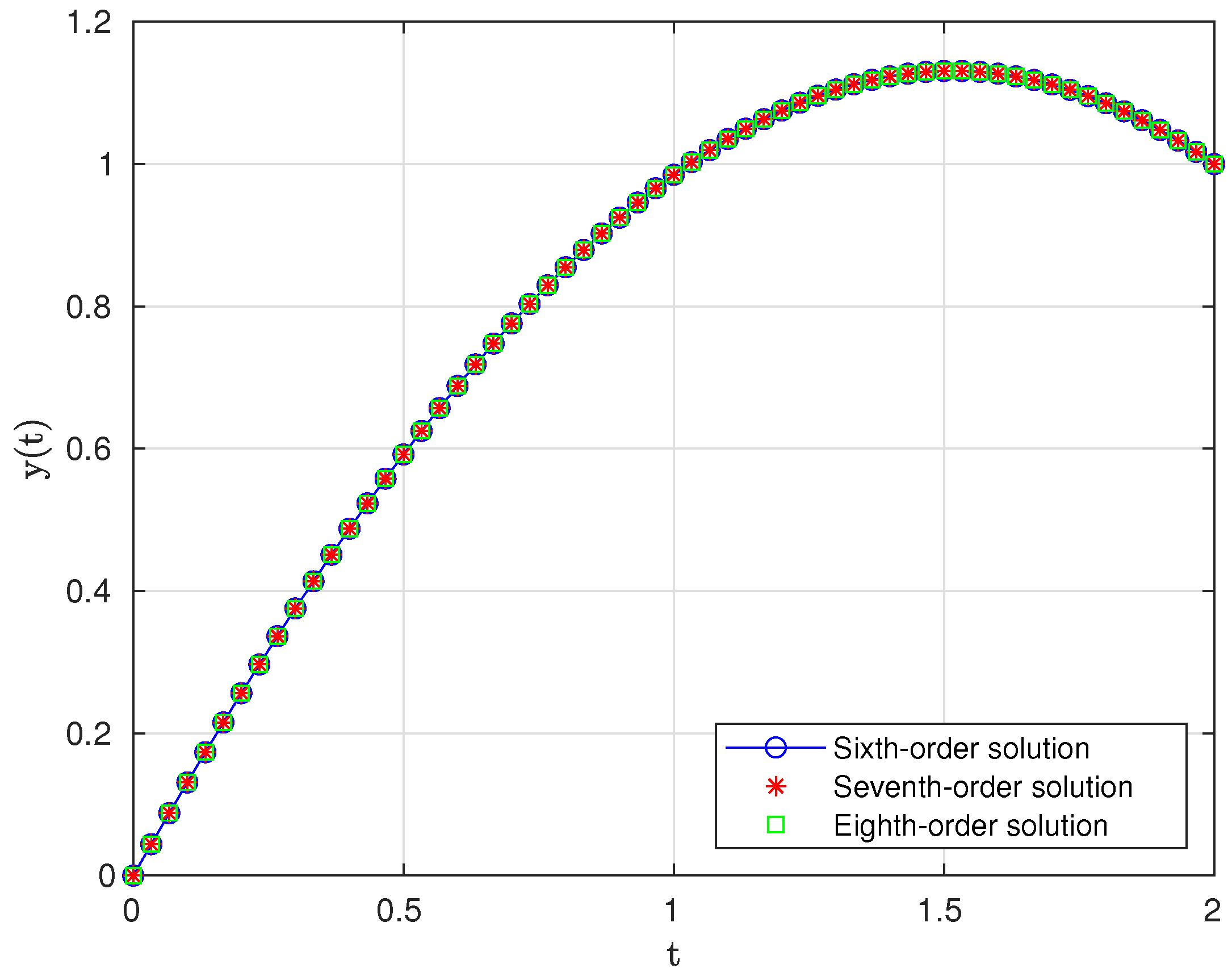
Example 5.

Consider the Van der Pol equation [29], which is described as follows:

$$y^{″}-\kappa (y^2-1)y^{\prime }+y=0,\kappa >0,y\left(0\right)=0,y\left(2\right)=1.$$

(22)

We consider the nodes $t_j,0\le j\le m$ satisfying $t_0=0<t_1<t_2<\dots <t_m=2$, where $t_j-t_{j-1}={\displaystyle \frac{2}{m}},j\ge 1$, and write, $y_0=y\left(t_0\right)=0,y_1=y\left(t_1\right),\dots ,y_{m-1}=y\left(t_{m-1}\right)$, $y_m=y\left(t_m\right)=1$. When we use the divided difference technique to discretize (22), we end up with a $(m-1)\times (m-1)$ system of nonlinear equations as follows:

$$4y_j-\kappa m(y_j^2-1)(y_{j+1}-y_{j-1})+m^2(y_{j-1}-2y_j+y_{j+1})=0,j=1,2,\dots ,m-1.$$

Let us take the value of $m=60$, initial approximation ${\displaystyle y_j^0=log\left({\displaystyle \frac{1}{j^2}}\right),j=1,2,\cdots ,59}$, and $\kappa ={\displaystyle \frac{1}{3}}$. For this case, we obtain a $59\times 59$ system of nonlinear equations. The graph of the approximated solution of (22) corresponding to the choices of $z_n$ as in (18)–(20) is plotted in Figure 1.

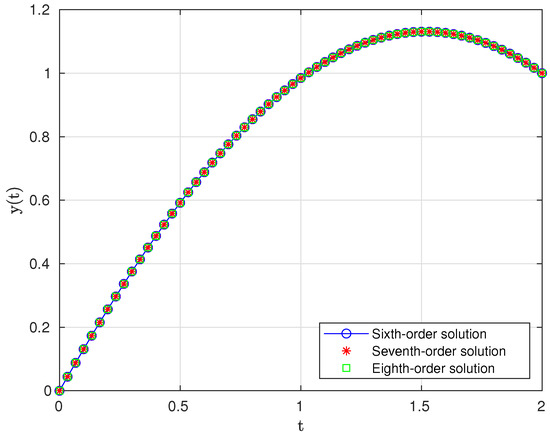
It is observed that from the Figure 1, the solution curve of the Van der Pol Equation (22) is concave on $[0,2]$.

5. Basin of Attractions

This section discusses the basin of attraction of a solution of the nonlinear system of Equation (1), considering $X=Y=\mathbb{C}$ with the usual norm. Let ${\displaystyle F:\widehat{\mathbb{C}}=\mathbb{C}\cup \{\infty \}\to \widehat{\mathbb{C}}}$ be an iterative function for (1). A point $\xi \in \mathbb{C}$ is called an attracting fixed point of F if it satisfies $F\left(\xi \right)=\xi$ and $|F^{\prime }\left(\xi \right)|<1$. We denote $F^n$ the n-time composition of F. For an iterative method, suppose that the sequence ${\left\{F^n\left(x_0\right)\right\}}_{n\ge 0}$ converges to the solution $\xi$; then, any such point $x_0$ is often referred to as an initial point/initial guess. The difficulty lies in making the correct initial guess. The set

$$\mathcal{A}\left(\xi \right)=\left\{x\in \widehat{\mathbb{C}}:{\left\{F^n\left(x\right)\right\}}_{n\ge 0}\mathrm{converges}\mathrm{to}\mathrm{a}\mathrm{solution}\xi \mathrm{of}\left(1\right)\right\}$$

is known as the basin of attraction of $\xi$. Such a set is always open but not connected in general. The connected component of $\mathcal{A}\left(\xi \right)$ containing $\xi$ is called an immediate basin of $\xi$. The set of correct guesses is precisely the union of all the basins corresponding to solutions of (1). The Fatou set is denoted by

$$\mathcal{F}\left(F\right)=\left\{x\in \widehat{\mathbb{C}}:{\left\{F^n\left(x\right)\right\}}_{n\ge 0}\mathrm{is}\mathrm{equicontinuous}\right\}$$

and the complement of $\mathcal{F}\left(F\right)$, denoted by $\mathcal{J}\left(F\right)$, is known as the Julia set. Here, $\mathcal{F}\left(F\right)$ is an open set, and $\mathcal{J}\left(F\right)$ is a closed set. For any attracting fixed point $\xi$ of F, we have $\mathcal{A}\left(\xi \right)\subset \mathcal{F}\left(F\right)$ and the boundary of $\mathcal{A}\left(\xi \right)$, $\partial \mathcal{A}\left(\xi \right)\subset \mathcal{J}\left(F\right)$. For more details, see [30,31,32,33,34,35].

Example 6.

Consider the following two complex-variable polynomials

$$\begin{array}{ccc}\hfill P\left(z\right)& =& z(z^3-1)\hfill \end{array}$$

(23)

$$\begin{array}{ccc}\hfill Q\left(z\right)& =& z(z-0.5)\left({(z-1)}^2+1\right).\hfill \end{array}$$

(24)

Note that the zeros for P are $z_0=0$, $z_1=1$, $z_2=-{\displaystyle \frac{1}{2}}+{\displaystyle \frac{\sqrt{3}}{2}}i$, and $z_3=-{\displaystyle \frac{1}{2}}-{\displaystyle \frac{\sqrt{3}}{2}}i$, and for Q, they are $z_0=0, z_1=0.5, z_2=1-i$, and $z_3=1+i$. We divide the region $R=\left\{z=x+iy|-2\le Re(z)\le 2,-2\le Im(z)\le 2\right\}$ which contains all the roots of (23), in $401\times 401$ equally spaced grid points. Next, we apply method (3) with $z_n$ as in (18)–(20) using each grid point as the initial point and obtain the basin of attractions for the roots $z_0,z_1,z_2$ and $z_3$ as shown in Figure 2 for (23) and Figure 3 for (24).

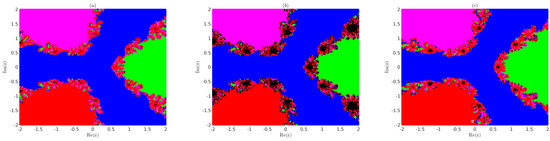
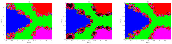
Note that we assigned the colours blue, green, magenta, and red to the grid points for which the sequence ${\left\{F^n\right\}}_{n\ge 0}$ converges. It converges with an accuracy of ${10}^{-8}$ to the roots $z_0$, $z_1$, $z_2$, and $z_3$, respectively. We assigned a black colour to divergent grid points in Figure 2 and Figure 3. It is observed from Figure 2 and Figure 3 that the convergence region for choice (19) is smaller than the convergence region of choices (18) and (20) of method (3) in R.

6. Conclusions

In this work, we extended the convergence order to $p+3$ from a two-step iterative method of order p using weaker conditions than in earlier studies. Numerical examples were discussed, and the performance of the considered methods was compared with some existing methods. From Equation (9), one could obtain a bound for the asymptotic error constant as $\zeta \left(r\right)$. Our work is limited to the operators which satisfy conditions $\left(C_1\right)$–$\left(C_6\right)$ only. Therefore, there is a scope to weaken these conditions further to enhance the applicability of the considered methods.

References

1. Sakawa, Y. Optimal control of a certain type of linear distributed-parameter systems. IEEE Trans. Automat. Control 1966, 11, 35–41. [Google Scholar] [CrossRef]
2. Hu, S.; Khavanin, M.; Zhuang, W. Integral equations arising in the kinetic theory of gases. Appl. Anal. 1989, 34, 261–266. [Google Scholar] [CrossRef]
3. Cercignani, C. Nonlinear problems in the kinetic theory of gases. In Trends in Applications of Mathematics to Mechanics (Wassenaar, 1987); Springer: Berlin/Heidelberg, Germany, 1988; pp. 351–360. [Google Scholar]
4. Lin, Y.; Bao, L.; Jia, X. Convergence analysis of a variant of the Newton method for solving nonlinear equations. Comput. Math. Appl. 2010, 59, 2121–2127. [Google Scholar] [CrossRef]
5. Grosan, C.; Abraham, A. A New Approach for Solving Nonlinear Equations Systems. IEEE Trans. Syst. Man Cybern.-Part A Syst. Humans 2008, 38, 698–714. [Google Scholar] [CrossRef]
6. Moré, J.J. A collection of nonlinear model problems. In Computational Solution of Nonlinear Systems of Equations. Lectures in Applied Mathematics; American Mathematical Society: Providence, RI, USA, 1990; Volume 26, pp. 723–762. [Google Scholar]
7. Argyros, I.K. Convergence and Applications of Newton-Type Iterations; Springer Science & Business Media: Berlin/Heidelberg, Germany, 2008. [Google Scholar]
8. Behl, R.; Arora, H. CMMSE: A novel scheme having seventh-order convergence for nonlinear systems. J. Comput. Appl. Math. 2022, 404, 113301. [Google Scholar] [CrossRef]
9. Lotfi, T.; Bakhtiari, P.; Cordero, A.; Mahdiani, K.; Torregrosa, J.R. Some new efficient multipoint iterative methods for solving nonlinear systems of equations. Int. J. Comput. Math. 2015, 92, 1921–1934. [Google Scholar] [CrossRef]
10. Cordero, A.; Leonardo-Sepúlveda, M.A.; Torregrosa, J.R.; Vassileva, M.P. Increasing in three units the order of convergence of iterative methods for solving nonlinear systems. Math. Comput. Simul. 2024, 223, 509–522. [Google Scholar] [CrossRef]
11. George, S.; Bate, I.; Muniyasamy, M.; Chandhini, G.; Senapati, K. Enhancing the applicability of Chebyshev-like method. J. Complex. 2024, 83, 101854. [Google Scholar] [CrossRef]
12. George, S.; Kunnarath, A.; Sadananda, R.; Jidesh, P.; Argyros, I.K. On obtaining order of convergence of Jarratt-like method without using Taylor series expansion. Comput. Appl. Math. 2024, 43, 243. [Google Scholar] [CrossRef]
13. Muniyasamy, M.; Chandhini, G.; George, S.; Bate, I.; Senapati, K. On obtaining convergence order of a fourth and sixth order method of Hueso et al. without using Taylor series expansion. J. Comput. Appl. Math. 2024, 452, 116136. [Google Scholar]
14. Ostowski, A.M. Solution of Equations and System of Equations; Academic Press: New York, NY, USA, 1960. [Google Scholar]
15. Weerakoon, S.; Fernando, T. A variant of Newton’s method with accelerated third-order convergence. Appl. Math. Lett. 2000, 13, 87–93. [Google Scholar] [CrossRef]
16. Cordero, A.; Martínez, E.; Torregrosa, J.R. Iterative methods of order four and five for systems of nonlinear equations. J. Comput. Appl. Math. 2009, 231, 541–551. [Google Scholar] [CrossRef]
17. Petković, M.S.; Neta, B.; Petković, L.D.; Džunić, J. Multipoint methods for solving nonlinear equations: A survey. Appl. Math. Comput. 2014, 226, 635–660. [Google Scholar] [CrossRef]
18. Argyros, I.K. The Theory and Applications of Iteration Methods, 2nd ed.; CRC Press: Boca Raton, FL, USA, 2022. [Google Scholar]
19. Cordero, A.; Gómez, E.; Torregrosa, J.R. Efficient high-order iterative methods for solving nonlinear systems and their application on heat conduction problems. Complexity 2017, 1, 6457532. [Google Scholar] [CrossRef]
20. Kelley, C.T. Approximation of solutions of some quadratic integral equations in transport theory. J. Integral Equ. 1982, 4, 221–237. [Google Scholar]
21. Hernández-Verón, M.A.; Martínez, E.; Singh, S. On the Chandrasekhar integral equation. Comput. Math. Methods 2021, 3, e1150. [Google Scholar] [CrossRef]
22. Burridge, R.; Knopoff, L. Model and theoretical seismicity. Bull. Seismol. Soc. Amer. 1967, 57, 341–371. [Google Scholar] [CrossRef]
23. van der Pol, B. The nonlinear theory of electric oscillations. Proc. IRE 1934, 22, 1051–1086. [Google Scholar] [CrossRef]
24. FitzHugh, R. Impulses and Physiological States in Theoretical Models of Nerve Membrane. Biophys. J. 1961, 1, 445–466. [Google Scholar] [CrossRef]
25. Hernández, M. Chebyshev’s approximation algorithms and applications. Comput. Math. Appl. 2001, 41, 433–445. [Google Scholar] [CrossRef]
26. George, S.; Sadananda, R.; Padikkal, J.; Argyros, I.K. On the Order of Convergence of the Noor–Waseem Method. Mathematics 2022, 10, 4544. [Google Scholar] [CrossRef]
27. Ham, Y.; Chun, C. A fifth-order iterative method for solving nonlinear equations. Appl. Math. Comput. 2007, 194, 287–290. [Google Scholar] [CrossRef]
28. Grau-Sánchez, M.; Grau, À.; Noguera, M. On the computational efficiency index and some iterative methods for solving systems of nonlinear equations. J. Comput. Appl. Math. 2011, 236, 1259–1266. [Google Scholar] [CrossRef]
29. Behl, R.; Cordero, A.; Motsa, S.S.; Torregrosa, J.R. Stable high-order iterative methods for solving nonlinear models. Appl. Math. Comput. 2017, 303, 70–88. [Google Scholar] [CrossRef]
30. Amat, S.; Busquier, S.; Plaza, S. Review of some iterative root-finding methods from a dynamical point of view. Sci. Ser. A Math. Sci. 2004, 10, 3–35. [Google Scholar]
31. Varona, J.L. Graphic and numerical comparison between iterative methods. Math. Intell. 2002, 24, 37–46. [Google Scholar] [CrossRef]
32. Campos, B.; Canela, J.; Vindel, P. Dynamics of Newton-like root finding methods. Numer. Algorithms 2023, 93, 1453–1480. [Google Scholar] [CrossRef]
33. Husain, A.; Nanda, M.N.; Chowdary, M.S.; Sajid, M. Fractals: An Eclectic Survey, Part-I. Fractal Fract. 2022, 6, 89. [Google Scholar] [CrossRef]
34. Husain, A.; Nanda, M.N.; Chowdary, M.S.; Sajid, M. Fractals: An Eclectic Survey, Part-II. Fractal Fract. 2022, 6, 379. [Google Scholar] [CrossRef]
35. Laplante, P.A.; Laplante, C. Introduction to Chaos, Fractals and Dynamical Systems; World Scientific: London, UK, 2023. [Google Scholar]
Figure 1. Graph of the solutions of (22).
Axioms 13 00601 g001
Figure 2. Basin of attractions of method (3) with z n as in (18)–(20), respectively, for (23).
Axioms 13 00601 g002
Figure 3. Basin of attractions of method (3) with z n as in (18)–(20), respectively, for (24).
Axioms 13 00601 g003