Abstract
In this research, we introduce the intuitionistic hesitant fuzzy rough set by integrating the notions of an intuitionistic hesitant fuzzy set and rough set and present some intuitionistic hesitant fuzzy rough set theoretical operations. We compile a list of aggregation operators based on the intuitionistic hesitant fuzzy rough set, including the intuitionistic hesitant fuzzy rough Dombi weighted arithmetic averaging aggregation operator, the intuitionistic hesitant fuzzy rough Dombi ordered weighted arithmetic averaging aggregation operator, and the intuitionistic hesitant fuzzy rough Dombi hybrid weighted arithmetic averaging aggregation operator, and demonstrate several essential characteristics of the aforementioned aggregation operators. Furthermore, we provide a multi attribute decision-making approach and the technique of the suggested approach in the context of the intuitionistic hesitant fuzzy rough set. A real-world problem for selecting a suitable worldwide partner for companies is employed to demonstrate the effectiveness of the suggested approach. The sensitivity analysis of the decision-making results of the suggested aggregation operators are evaluated. The demonstrative analysis reveals that the outlined strategy has applicability and flexibility in aggregating intuitionistic hesitant fuzzy rough information and is feasible and insightful for dealing with multi attribute decision making issues based on the intuitionistic hesitant fuzzy rough set. In addition, we present a comparison study with the TOPSIS approach to illustrate the advantages and authenticity of the novel procedure. Furthermore, the characteristics and analytic comparison of the current technique to those outlined in the literature are addressed.
Keywords:
intuitionistic hesitant fuzzy rough sets; Dombi aggregation operators; multi-attribute decision making; suitable multinational partnership MSC:
03E72
1. Introduction
Recently, a variety of approaches have emerged with the intention of tackling the complicated issues associated with decision making in an uncertain environment. Exploring the methodologies and concepts associated with decision making under conditions of uncertainty has consequently ignited an abundance of interest among researchers from a variety of disciplines. Ref. [1] introduced the idea of the fuzzy set (FS) as an approach for portraying situations demarcated by their unpredictability. In addition to computer science, medicine, clustering, robotics, optimisation, and data mining, the FS has been implemented in numerous professional fields. The range of values for the FS membership grade is [0, 1]. The nonmembership grade (NMG) of an element in FS is equal to , where represents its membership grade (MG). In the context of fuzzy sets, the degree of hesitancy is typically zero. Despite the significance FS attributes to the MG concept, the procedure for determining MG occurs with unpredictability. As with other theories, the FS theory provides a mathematical framework for coping with uncertain situations. Nevertheless, it is imperative for recognising that this approach has its constraints, predominantly attributable to the intricacy of substantial DM challengers. The continued appearance of these issues suggests that DM platforms for interaction be broadened and diversified. To enhance the applicability of fuzzy set theory, the notion of an intuitionistic fuzzy set (IFS) is introduced by [2]. The IFS is an incredibly beneficial tool for classifying complex ambiguous information by integrating the membership grade and non-membership grade notions instantly. This provides greater flexibility in handling situations of uncertainty and ambiguity. In IFS, the sum of MG and NMG does not exceed 1, i.e., . Still, the viability of IFS implementations is constrained due to conceivable situations where decision makers (DMs) may encounter circumstances in which the sum of MG and NMG exceeds one. There are numerous circumstances in which the IFS is incapable of representing specific assessment information. Ref. [3] developed the novel idea of Pythagorean fuzzy sets (PFS), which might be helpful in tackling the problem of complexity. The PFS is the modified form of IFS and consists of sets where the square sum of the MG and NMG is less than or equal to 1. Despite this, the spiralling unpredictability of DM determinants and the conflicting points of view of decision makers make it difficult for PFS to overcome challenges in providing valuable knowledge. As a result, the functionalities of FSs, IFSs, and PFSs are restricted by constraints. The essential information monitoring tools keep on growing, and individuals increasingly have greater and more credibility with information to provide predictive insights on their own reliability. Considerable significance has been devoted to the desire of understanding in the field of artificial intelligence. This comprises a wide variety of initiatives (pattern extraction, natural language processing, data analysis, and so on).
1.1. A Brief Introduction to the Concept of Rough Sets
The concept of rough sets (RSs), innovated by [4], has emerged as a pivotal framework for effectively managing ambiguous, indistinguishable, and inadequate information and knowledge. The RS theory is an innovative mathematical framework designed to cope with ambiguous information in data processing. It is based upon the principles of scientific data theory, probability theory, and FS theory. The mathematical tool provided by the RS theory is for resolving equivocal situations and establishing two distinct boundaries within which complex ideas are capable of being articulated. The RS theory, which extends the crisp set theory, owns the domain of advanced information processing with a versatile, innovative, and accessible framework. A considerable amount of effort and time has been consigned by researchers in recent years to investigating innovative implementations of RS theory. These initiatives have culminated in notable improvements to the theory and detailed characterizations of its real-world applications in various domains, including computer vision, feature learning, data analysis, predictive modelling, and analysis (see [5,6] for detailed information). The notion of fuzzy RS was introduced by [7] through the substitution of fuzzy relations for crisp binary relations. The idea of IF rough sets developed by [8] is an innovative approach that merges the fundamental principles of IFS and RS. By establishing an intersection between the two theories, this integrated framework represents the upper approximations (UA) and lower approximations (LA) as IFSs, respectively. Ref. [9] initially reported the notion of IFS rough sets. Ref. [10] introduced the notion of precise and fuzzy approximation space to explicate the idea of approximate IFSs and IFRSs, respectively, in their research. Furthermore, an exhaustive evaluation of the restricted fundamental assessment of these systems was performed. A comprehensive examination was conducted by [11,12], who meticulously assessed and implemented the framework of a dominance-based IF rough set theory. The research innovated by [13] explored the assessment of a comprehensive notation that can be effectively employed in the exploration of numerous relation-based approximate approximation operators for IF. The focus of this analysis was the application of a particular form of the IF triangular norm throughout logical methodologies. The notion of combining FSs, RSs, and soft sets was developed by [14], and the integration of these constituents has played a pivotal role in the emergence of numerous pioneering notions involving the rough soft sets, soft RSs, and soft rough FSs. Several researchers have conducted investigations on the merging of soft sets and RS models (for more information see [15,16,17]). A comprehensive foundational framework for IFRS was introduced by [18], which significantly enhanced the fundamental principles of IF. The fundamental concepts of soft set and RS theories [19,20,21] are investigated within the framework of Pythagorean and orthopair FSs to provide a more extensive comprehension of IFS. The characteristics of various aggregation operators (AOPs) and their application in decision-making, particularly the use of trapezoidal IF numbers [22], are investigated in detail. The concept of triangular IF numbers [23] is addressed to assess their practical importance within the group DM framework. We evaluate numerous operational principles for IF approximation numbers based on the Aczel–Alsina theory discussed by [24]. Additionally, the study illustrated the significant role of AOPs in medical diagnostics and DM applications. The mathematical frameworks of spherical FSs, RSs, and soft sets [25] proposed an innovative concept known as spherical fuzzy soft rough sets. Numerous researchers investigated the crucial features of the established spherical fuzzy soft rough average AOPs. In order to improve DMs, the researchers [26] investigated and presented the implementation of ordered weighted average AOPs based on IFRSs.
1.2. A Brief Historical Overview of Dombi Aggregation Operators
The Dombi triangular-norm and Dombi triangular-conorm operations were introduced by Dombi in 1982 and have gained enormous popularity as the most widely used approach to handling variable operation variability. Employing the Dombi t-norm and t-conorm, Ref. [27] described the Dombi algebraic operations and performed on interval-valued hesitant FSs. Ref. [28] presented and addressed a variety of geometric AOPs and averaging AOPs based on the Dombi t-norm and t-conorm. The authors further elaborated on the implementation of these operators in DM scenarios. Dombi aggregation operators were proposed by [29] throughout the framework of spherical cubic fuzzy information. Multiple attribute decision making (MADM) was utilised to illustrate the validity, practicability, and efficacy of the proposed methodologies through the implementation of these operators. Ref. [30] examined the characteristics of spherical fuzzy Dombi AOPs and discussed their implementation in MADM problems. Ref. [31] proposed Dombi AOPs for single-valued neutrosophic information and described their utilisation in MADM problems. To resolve the DM challenge, Ref. [32] generalized the notion of the Dombi operation for neutrosophic cubic sets. Dombi AOPs for linguistic cubic variables were initially developed to tackle the MADM problem by [33]. Ref. [34] established and employed Dombi AOPs based on hesitant fuzzy information for typhoon catastrophe assessment in 2018. Ref. [35] assembled a variety of Dombi AOPs based on picture FSs and assessed their real-world acceptance in portfolio management.
1.3. A Comprehensive Overview of the TOPSIS Method
The technique for order of preference by similarity to ideal solution (TOPSIS), which is widely recognised as the most prominent MADM analysis approach, was established by [36]. It is implemented to address prudent DM challenges. In accordance with the TOPSIS method, the optimal alternative is defined as the one that portrays the greatest distance from the negative ideal solution (NIS) and the smallest distance from the positive ideal solution (PIS). A more accurate comparison of multiple alternatives can be achieved by assigning weights to each criterion. This technique is crucial for DM problems, as MADM scenarios involve a wider range of conflict criteria. Ref. [37] proposed an enhancement to the TOPSIS method through the implementation of a distance measure constructed using interval type-2 trapezoidal Pythagorean fuzzy numbers. They subsequently investigated the potential applications of this method for addressing MADM challenges, contemplating an assessment of the perspectives and views of decision makers. The optimal parameters were identified, categorised, and evaluated by [38] using the analytic hierarchy process (AHP) and TOPSIS approaches. Ref. [39] introduced an innovative approach to organisation ranking for group DM using ordered fuzzy integers and the TOPSIS method. Ref. [40] formulated a technique to tackle the challenge of identifying sustainable partners through the utilisation of DM professionals who were previously indistinguishable. Ref. [41] presented the TOPSIS method in a scenario with undetermined attribute and decision-maker weights based on interval Pythagorean fuzzy numbers. Furthermore, the interval Pythagorean fuzzy number is utilised to consolidate the evaluation matrices provided by a large number of decision makers into a global evaluation matrix. To demonstrate the efficacy and rationality of the suggested approach, a real-world example is provided. Ref. [42] established a novel TOPSIS DM approach by employing IFSs, interval FSs, and additional types of assessment information. Ref. [43] developed TOPSIS, an innovative technique for implementing decision-theoretic rough FSs. They demonstrated the stability and superiority of the proposed technique via bench-marking and parameter assessment. In addition, real-world DM assessments were performed to validate the proposed methodology.
1.4. A Short Introduction of HFSs
The notion of hesitant FSs (HFSs), initially introduced by [44], provides an effective characterization tool for the fuzziness associated with human perception and the ambiguity that prevails in complex situations. Considering their inception, significant strides have been made in both the theory and application of HFSs. Ref. [45] carried out an analysis on the multidimensional consistency of fuzzy preference relations. A novel approach utilising HFSs is proposed by [46] to address attribute selection in MADM scenarios involving high-dimensional sets of information. Sun et al. Ref. [47] proposed a novel approach to pattern recognition challenges with HFSs by utilising grey relational assessment. Ref. [48] assessed the efficacy of a novel MADM technique in the framework of HFSs and its implications for energy policy initiatives by employing the TOPSIS approach. An MADM procedure based on the possibility theory was described and investigated by [49] for implementation in the environment involving hesitant and ambiguous syntax. Recently, there has been considerable interest in acquiring additional understanding regarding hybrid models that are ascribed as merging RSs theories [50,51] with HFSs [44]. Ref. [52] introduced the notion of a hesitant fuzzy set and rough set. Both constructive and axiomatic strategies were taken into consideration. Furthermore, they assessed a hesitant fuzzy destination by employing a hesitant fuzzy relation and discussed the main goal of the model. The axiomatic method provides a description of hesitant fuzzy rough set utilizing operators. Hesitant fuzzy rough approximation operators are precisely specified via the use of axioms. By using distinct sets of axioms for lower and upper hesitant fuzzy set theoretic operators, it is possible to establish various types of hesitant fuzzy relations. Ref. [53] put forward the notion of a hesitant fuzzy RS, which is comprised of two distinct universes. They explored the potential utilization of this set in the field of DM. Owing to its implementation, it simulates more accurately the complexities of decision-making in the real world when two separate interconnected universes are considered.
1.5. The Motivations of the Manuscript
The above-mentioned research initiatives, hybrid models that combine an IFSs with RSs are rarely assembled. A couple of innovative frameworks in fuzzy rough set theory have been effectively developed through the integration of a Pawlak rough set with a variety of other uncertainty theories, such as FS, IFS, PFS, soft set theory, and many more. The idea of IFRSs is also an important framework to cope with uncertain information, and we found a lack of hesitation. The aforementioned literature aroused our interest in constructing a distinctive notion of intuitionistic hesitant fuzzy rough sets (IHFRSs) by integrating HFSs and IFRSs and exploring how it may be employed in an MADM challenge in a hesitant fuzzy environment. The motivations for the present manuscript are as follows:
- (1)
- To compile a list of numerous AOPs based on Dombi t-norm and t-conorm, namely, IHFR Dombi weighted averaging aggregation operator (IHFRDWAAO), IHFR ordered weighted averaging aggregation operator (IHFRDOWAAO), and IHFR Dombi hybrid weighted averaging aggregation operator (IHFRDHWAAO), and investigate their key operating laws. Additionally, describe their related properties.
- (2)
- To establish the score and accuracy functions employing IHFRSs.
- (3)
- To provide a DM technique for combining vague information employing the prescribed AOPs.
- (4)
- By using the demonstrated AOPs, an empirical analysis using numerical information from a real-world DM problem involving the selection of a suitable multinational partnership is initiated.
- (5)
- The findings are also assessed using comparisons to the IHFR-TOPSIS approach.
1.6. Structure of the Article
The remaining part of the presented research is outlined as follows: Section 2 provides a concise overview of the information essential to several fundamental concepts. Section 3 defines the Dombi t-norm and t-conorm and its based AOPs. Section 4 shows the MADM approaches utilising IHRFR information. Section 5 depicts a real-world DM application for selecting a worldwide partnership. Section 6 and Section 7 demonstrate the sensitivity analysis and comparison assessment, respectively. Finally, Section 8 summarises the findings and suggests potential approaches for further exploration.
2. Basic Concepts
This part contains some significant fundamental information, including FS, HFS, IFS, IHFS, RS, IFRS, and IHFRS, as well as an overview of operational laws that are associated with these concepts. The reader will be more knowledgeable to perceive the proposed framework with an understanding of the following basic ideas.
Definition 1
([1]). Introduced the idea of FS. Let be a universal set. Then, FS F on ℑ is outlined as
where , called the MG.
Definition 2
([54]). Developed the concept of HFS. Let be a universal set. Then HFS H on is characterised as
where is a set of values comprising which shows the MG of The element of is recognised as the HF element.
Definition 3
([2]). Innovated the notion of IFS. Let be a universal set. An IFS ϝ over is expressed as
for each , the functions , and show the MG and NMG, respectively, which must satisfy the property
Definition 4
([55]). Introduced the concept of intuitionistic hesitant FS (IHFS). An intuitionistic hesitant FS (IHFS) E over a universal set is characterised as follows:
where ϱi and ϱi are two sets of some values in that symbolise the MG and NMG accordingly. The conditions that are required are as follows: , , with the property that and
Definition 5
([4]). Developed the idea of the rough set. Let be a universal set, and be and arbitrary relation on Define a set value mapping by for where is called a successor neighbourhood of the element with respect to relation The pair is called crisp approximation space. Now, for any set the LA and UA of with respect to the space are stated as
where are upper and lower approximation operators, and the pair is identified as RS.
Definition 6.
Let be the universal set, and be an IF relation. Then
- (1)
- is reflexive if and
- (2)
- is symmetric if , and
- (3)
- is transitive if
Definition 7
([56]). initiated the idea of IF rough set. Let be the universal set. Then any relation is called IF relation. The pair is said to be IF approximation space. Now, for any , the LA and UA of with respect to IF approximation space are two IFSs and symbolised by and , which is highlighted below:
and
where
such that
As are so are LA and UA operators. The pair
is identified as an IF rough set. For simplicity
is represented as and is known as IFR value.
Definition 8.
Let ℑ be the universal set. Then, for any subset, is said to be an IHF relation. The pair is said to be an IHF approximation space. If, for any , then the LA and UA of with respect to the IHF approximation space are two IHFSs, which are displayed by and and expressed as
and
where
such that and As are so are LA and UA operators. The pair
shall be recognised as intuitionistic hesitant fuzzy RSs (IHFRSs). For simplification
is portrayed as and is designated as an IHFRS value.
Definition 9.
The scoring function employed for the IHFRV is given by:=
The accuracy function for IHFRV is given as
where and symbolises the number of elements in and respectively.
Definition 10.
Suppose and are two q-ROHFRVs. Then
- (1)
- If then
- (2)
- If then
- (3)
- If then
- (a)
- If then
- (b)
- If then
- (c)
- If then
3. Dombi Aggregation Operators Based on Intuitionistic Hesitant Fuzzy Rough Sets
3.1. Dombi t-Norm and t-Conorm
This portion describes the Dombi product and Dombi sum described by [57] in detail and discusses certain fundamental operations based on IHFRSs that are useful for the subsequent analysis. These are particular kinds of triangular norms and co-norms.
Definition 11
([57]). Let and be two real numbers that comprise the interval [0, 1]. Then, Dombi t-norm is portrayed by
3.2. Dombi Operations of IHFR Information
In this subsection, we define some Dombi operations between IHFRSs.
Definition 12.
Let = and = be two IHFRSs and Then, the Dombi operations for IHFR numbers are outlined below:
3.3. Aggregation Operators
The Dombi weighted arithmetic averaging operator, Dombi ordered weighted arithmetic averaging AOPs, and Dombi hybrid weighted arithmetic averaging AOPs are initiated in this section.
3.4. Intuitionistic Hesitant Fuzzy Rough Dombi Weighted Arithmetic Averaging (IHFRDWAA) Operator
Let = be an n-dimensional of IHFRSs. An IHFRDWAA operator is defined by the function IHFRDWAA: as follows:
where is a weight vector of ), and
Theorem 1.
Let ). Then
where is a weight vector of ), , and
Proof.
Refer to the Appendix A for the proof of Theorem 1. For explanation of the above concept of the IHFRDWAA operator, we present the following example. □
Example 1.
Let
For and with weight vector we obtain
Theorem 2.
(Idempotency): Let be a number of IHFRNs and
be an equal number to the IHFR element, i.e., for all ı. Then IHFRDWAA.
3.5. Intuitionistic Hesitant Fuzzy Rough Dombi Ordered Weighted Arithmetic Averaging (IHFRDOWAA) Operator
Let
be an n-dimensional of HFRSs. An IHFRDOWAA operator is defined by the function IHFRDOWAA: , as follows:
where is the largest of , and is weight vector of ), such that and
Theorem 3.
Let ). Then,
where is the largest of , and is the weight vector of ), such that and
Proof.
The proof is straightforward and similar to the proof of Theorem 1. □
3.6. Intuitionistic Hesitant Fuzzy Rough Dombi Hybrid Weighted Arithmetic Averaging (IHFRDHWAA) Operator
Let = be an n-dimensional of IHFRSs, and let be the associated weight vector such that and . The weight vector of ), such that and . An IHFRDHWAA operator is defined by the function IHFRDHWAA: , as follows:
Theorem 4.
Let ). Then
where shows that the value of the permutation obtained from the set of IHFRVs is superior, in which n indicates the balancing coefficient.
Proof.
The proof is straightforward and identical to the proof of Theorem 1. □
4. Multiple Attribute Group Decision-Making Method under IHRFR Information
The MADM is a very significant procedure to select an ideal alternative within the range of favourable options based on the viewpoints of some professionals corresponding to attributes. An expert panel evaluates each alternative according to the common attributes and presents a recommendation in the form of an IHFRV for each attribute. The obtained information in the decision matrices from the experts is aggregated by using their weights. Then, the obtained aggregated information is aggregated for the collective aggregated value of each alternative through implementation of the provided weights of the attributes. The MADM is a very useful technique in several fields. It is widely used in business, economics, mathematics, engineering, and so on. In this section, we construct a MADM methodology, including the following key steps:
- Step-1
- Let be the set of alternatives, be the set of criteria, and be the set of decision-makers with the weight vector where such that . The MADM method comprises the following procedures:
- Step-2
- The assessment of the alternative based on criteria by decision makers can be written as . Consequently, the IHFR decision matrix DMAi may be established as follows:
- Step-3
- Assess the normalised expert matrices as
- Step-4
- Construct the collected IHFR information using IHFRDWAA related to , denoted by , as follows:
- Step-5
- To use the aforementioned aggregation information, assess the combined IHFR values for each alternative that has been investigated in accordance with the specified list of attributes/criteria.
- Step-6
- Compute the score values for
- Step-7
- Assemble the numerical values of all score values in a specific sequence.
- Step-8
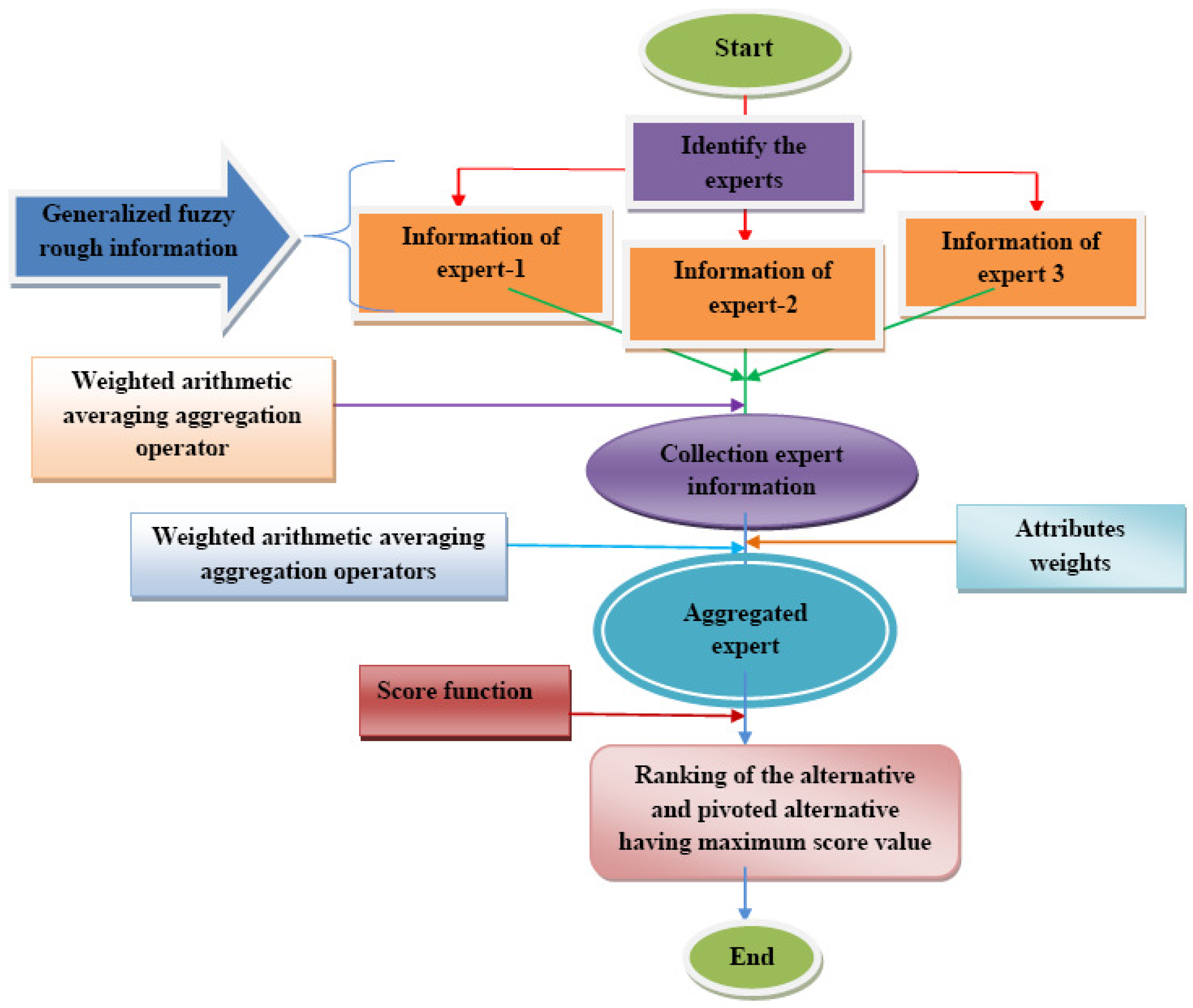
- Select the option retaining the highest scoring value. Figure 1 illustrates the diagrammatic chart of the algorithm for the implied MADM technique.
 Figure 1. Illustration of the flowchart for suggested MADM algorithm.
5. Numerical Application
In this part, we provide an MADM problem to illustrate the effectiveness and versatility of the mentioned technique. Since the globalisation of the international economy causes organisations to confront increasingly complex environments both externally and internally, selecting a good partner is an important approach to maintain consistent competitiveness, which may be impacted by a variety of circumstances. The global partnership (GP) is a collaboration of businesses and organisations working together to address sustainability challenges by sharing knowledge and implementing development ventures. The GP for the environment and sustainable growth cooperation is a multi-stakeholder platform that aims to improve the efficacy of development efforts by all partners, generate long-term outcomes, and promote the accomplishment of the sustainable development goals. The 2030 Agenda for sustainable growth cannot be realised unless all the available development resources from all stakeholders are gathered and strategically employed. Authorities, multilateral and bilateral organisations, non-profits, companies, legislators, and labour leaders have formed the GP for comprehensive development cooperation to enhance the significant consequence of international development. The GP emphasises effective development cooperation aimed at eradicating all manifestations of disparities and hunger, promoting sustainable development, and guaranteeing that everyone achieves the assistance they require. It involves practical assistance and information dissemination to increase development impact and promoting nation achievement of core international development effectiveness principles. Herein, we considered four factors, which are research and technology development capacity, business operation level, international cooperation level, and credit level.
- (i)
- Science, technology, and innovation (STI) (): Science, technology, and innovation have long been recognised as a fundamental resource in productivity growth and a significant, long-term strategy for increasing economic development and living standards. If developing countries are to be capable of participating in international STI activities, humanitarian assistance should collaborate more intimately with research and innovation stakeholders to strengthen STI capability. As a consequence, it is essential to promote more production capacities by both governments and corporations, particularly via public–private partnerships. Moreover, it is critical to collaborate in order to build the skills required to capitalise on the opportunities given by STI in the pursuit of sustainable development. Because of the interaction of science, technology, innovation, and digitalisation, tremendous upheavals are feasible. Until now, it has been probable that these changes would not immediately alleviate social and environmental challenges. Essentially, changing global development onto a more sustainable route will need not only the extension of currently appropriate technology but also radical breakthroughs (including social ones) and paradigm transformations. The capacity to innovate is important because desired adjustments in attitudes and practises need (social) innovation. Ultimately, STI may become a common goal of the public and private sectors, mobilising all investments in the direction of sustainable development, and it may be structured towards industries that cause economic and social changes, all of which minimise transformation costs.
- (ii)
- Business operation level (): Business operations are the ordinary activities that a corporation performs in order to increase its value and produce revenue. It is conceivable to optimise operations to the point that they produce greater profits than they consume. Employees contribute to a company’s success by performing crucial duties such as advertising, accounting, and production. As a firm grows, it must alter its operating procedures to keep things running smoothly, which requires meticulous planning on the part of senior management. A growing organisation must be equipped to confront new challenges such as those connected to the law, marketing, and growth. A corporation should develop effective and quantifiable measures to monitor its success. Establishing goals is the first step towards generating a foundation for performance assessment. Management should strive for clear, quantifiable results. Keeping up with industry advances is essential for discovering cost-cutting and productivity-boosting possibilities, as well as satisfying the needs of evolving policies. Another strategy for improving the efficiency of company operations is to keep up with industry advances. Management should constantly be looking for alternative techniques to streamline and improve critical operations.
- (iii)
- International cooperation level (): The International cooperation level for the GP is the major multi-stakeholder vehicle for enhancing development effectiveness by increasing the efficacy of all types of development cooperation for the shared tangible benefits for individuals, the environment, prosperity, and harmony. It brings together groups devoted to improving the effectiveness of their development relationships, including governmental institutions, non-governmental organisations, businesses, parliamentarians, and labour organisations. A binding contract is formed between two or more parties to share resources and collaborate to accomplish a common goal. National stakeholders and external partners (such as international development organisations) must take part in the establishment, implementation, and assessment of a country’s own development strategy under the guidance of the government. Commitment is reflected when public or private institutions work together to achieve mutual goals or adopt common procedures, such as in scientific endeavours or the establishment of mandatory industry standards.
- (iv)
- Credit level (): In numerous countries, the principle of economic growth has been elevated to the level of a national policy priority. Private enterprises are intensifying their efforts to reach previously unserved or undeserved aspects as a consequence of decision makers’ and regulators’ attempts to improve the level of financial inclusion in their countries. Formerly, conceptions of financial inclusion have differed significantly among countries; however, there has been significant convergence in recent years. There is accessibility to a diverse choice of appropriate financial services (i.e., individuals, firms and government entities). These criteria include the desire to purchase and pay, as well as the usage of credit, credit cards, savings, investment, and insurance products and services. The quality of financial merchandise and services, when paired with consumer protection and financial knowledge, maximises a user’s capacity to realise the advantages when employing these products and services on a regular basis.
The Evaluation Procedure for Selecting an Appropriate Global Partnership
Suppose a corporation has nominated four candidate companies in the worldwide scope with the intention of selecting an optimal global partner. A panel of professionals across the globe has been invited to evaluate and determine the most acceptable partnership for the organisation. Let be a set of three decision-makers; the set of four alternatives is , and let be the set of four criteria where : Science, technology, and innovation; : business operation level; : international cooperation level; and : credit level. It should be noted that all of the attributes presented here are of the benefit type. The decision makers weight vector is = , and the associated attribute weight vector is = . In order to evaluate alternatives and analyse the MADM scenario employing the aforementioned approach, the subsequent operations are executed:
- Step-1
- The information reported in Table 1, Table 2 and Table 3 was obtained from three experts according to IHFRVs.
 Table 1. Expert-1 information.
Table 2. Expert-2 information.
Table 3. Expert-3 information.
Table 1. Expert-1 information.
Table 2. Expert-2 information.
Table 3. Expert-3 information. - Step-2
- There is no need for normalisation because all of the expert information is of the benefit type.
- Step-3
- Table 4 demonstrates the IHFRDWA evaluation of the accumulated information of three expert analysts. Based on the score value of the collected expert information displayed in Table 5, the ordered collected expert information is presented in Table 6.
Table 4. Collected expert information.
Table 5. Score values of collected expert information.
Table 6. Ordered collected expert information.
- Step-4
- Ascertain the aggregate IHFR values for each of the assessed alternatives using the specified set of criteria/attributes utilising the aggregation information. Table 7 and Table 8 visualised the aggregated information for IHFRDWA and IHFRODWA, respectively. The hybrid collected expert information is presented in Table 9, and their score values are displayed in Table 10. The results of IHFRHDWA are presented in Table 11.
Table 7. IHF rough aggregation information using IHFRDWA operator.
Table 8. IHF rough aggregation information using IHFRDOWA operator.
Table 9. Hybrid collected expert information.
Table 10. Score values of hybrid collected expert information.
Table 11. IHF rough aggregation information using IHFRDHWA operator.
- Step-5
- The score values determined for the information acquired via IHFRDWA, IHFRODWA, and IHFRHDWA are presented in Table 12. Ranking alternatives accordingly to their score, we observed that is the optimal alternative. The ranking of the score values of the acquired information through IHFRDWA, IHFRODWA, and IHFRHDWA is depicted in Figure 2.
Table 12. Ranking order of alternatives.
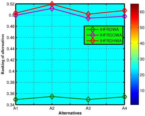 Figure 2. The graphical illustration of ranking order.
6. Sensitivity Analysis
It is clear that the IHFRDWAA consists of the parameter , due to which it becomes very flexible and significant in successfully dealing with imprecise information. In our example, the value of parameter = 1 is explored. We investigate the capability for variations in the outcomes obtained through the IHFRDWAA operator. The subsequent ranking orders are presented in Table 13 and Figure 3; the analyses are performed using the score values obtained through the IHFRDWAA operator. With the possible variation in the parameter , we identify multiple values from 1 to 5 and 1, 20, 50, 100 and sort out the IHFR score values in ascending order. The optimal alternative in the IHFRDWAA remains constant by varying the value of . In addition, it should be noted that the sequences of alternatives () remain unaltered by changing the value of . From the score value compilation through the IHFRDWAA operator, alternative was determined to be the optimal alternative, while alternative achieved the smallest achievable score values for = 1 to 5 and 1, 20, 50, 100, as illustrated in Table 13. Therefore, the most appropriate alternative is similar for the value of from 1 to 1. The graphical representation of Table 13 is illustrated in Figure 2. The impact of variation on the ranking order through employing the IHFRWAA operator is illustrated in Figure 3.
Table 13.
Ranking categorisation based on IHFRWAA operator for various values of .
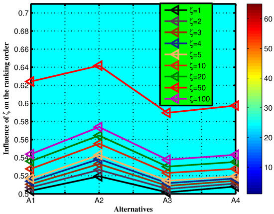
Figure 3.
The impact of on the order of ranking under the IHFRWAA operator.
7. Comparative Analysis
The TOPSIS strategy performs under the fundamental assumption that the degree of desirability of an alternative directly correlates with its distance from the negative ideal solution (NIS) and its proximity to the positive ideal solution (PIS). As a consequence, researchers have developed several techniques that are capable of completing the process of classifying alternatives in worldwide decision making problems. These algorithms are devoted to dealing with the ordering of feasible alternatives. We develop a novel TOPSIS methodology based on IHFRSs that handles the identification and categorisation of alternatives. By utilizing these criteria, we explain in detail how the innovative TOPSIS technique works and assess its validity. The feasibility of our technique is then verified using a sample project financial judgment; as well, its effectiveness and sustainability are shown via comparisons to alternative approaches and a variety of experiments with varying input parameters. In addition, we conduct a simulation experiment to test how our strategy compares to the traditional TOPSIS approach in terms of sorting attributes. TOPSIS is a framework employed by [36] for assessing the advantages and disadvantages of various policy approaches under ideal situations. The TOPSIS approach characterises the best possible decision as the one that relates closely to PIS for all of the criteria while simultaneously becoming the farthest away from the NIS, described by [58,59]. Several researchers have reviewed various types of MADM methods to achieve specific goals, and some researchers have conducted comparisons between different MADM methods by analysing real-life MCDM problems, as displayed in Table 14.
Table 14.
Comparison between several decision-making methods. (CT = computational time, MC = mathematical calculation, IT = information type).
The TOPSIS scheme consists of mainly the following steps:
- Step-1
- Let the set of alternatives be and the set of criteria be , and the information obtained from the professionals is provided as follows:whereandsuch thatare the IHFR rough values.
- Step-2
- First, we assemble information from DMs using IHFR numbers.
- Step-3
- Second, normalise the DM information, owing to the fact that the decision matrix contains cost and benefit criteria, which is demonstrated as follows:where shows the number of experts.
- Step-4
- Analyse the normalised information obtained from professionals as
- Step-5
- The PIS and NIS are determined by the score values. are the PIS and are the NIS. The algorithm that yields the PIS is as follows:In a comparable way, the formula used to determine the negative ideal solution is as follows:Based on the aforementioned information, calculate the geometric distance between each alternative and the PIS using the subsequent algorithm:Likewise, the geometric distance between each alternative and the NIS, represented as , can be expressed in the following mathematical manner:
- Step-6
- Here is the procedure employed for determining the relative closeness indices for each DM alternative:
- Step-7
- In the context of decision making, the alternative with the minimum distance is deemed the most preferable.
7.1. A Numerical Illustration
This section is devoted to presenting an MADM challenge that serves as an exemplification of the framework’s exceptional adaptability and enormous variety of applications, as well as a numerical illustration to choose the best international partner for a multinational company. The following is a summary of the key procedures:
- Step-1
- Step-2
- The collected expert information obtained using the IHFR Dombi weighted arithmetic averaging aggregation operator are presented in Table 4.
- Step-3
- There is no need to normalise the information since it is the benefit type.
- Step-4
- The PIS and NIS can be determined by referencing the score value, as displayed in Table 15.
Table 15. Ideal solutions.
- Step-5
- In order to determine the distance, measure between PIS and NIS as follows:
Distance measures of PIS 0.0483 0.0369 0.0311 0.0334 andDistance measures of NIS 0.0411 0.0539 0.0122 0.0419
- Step-6
- The procedure for determining the relative closeness indices for all DMs of the alternatives is as follows:
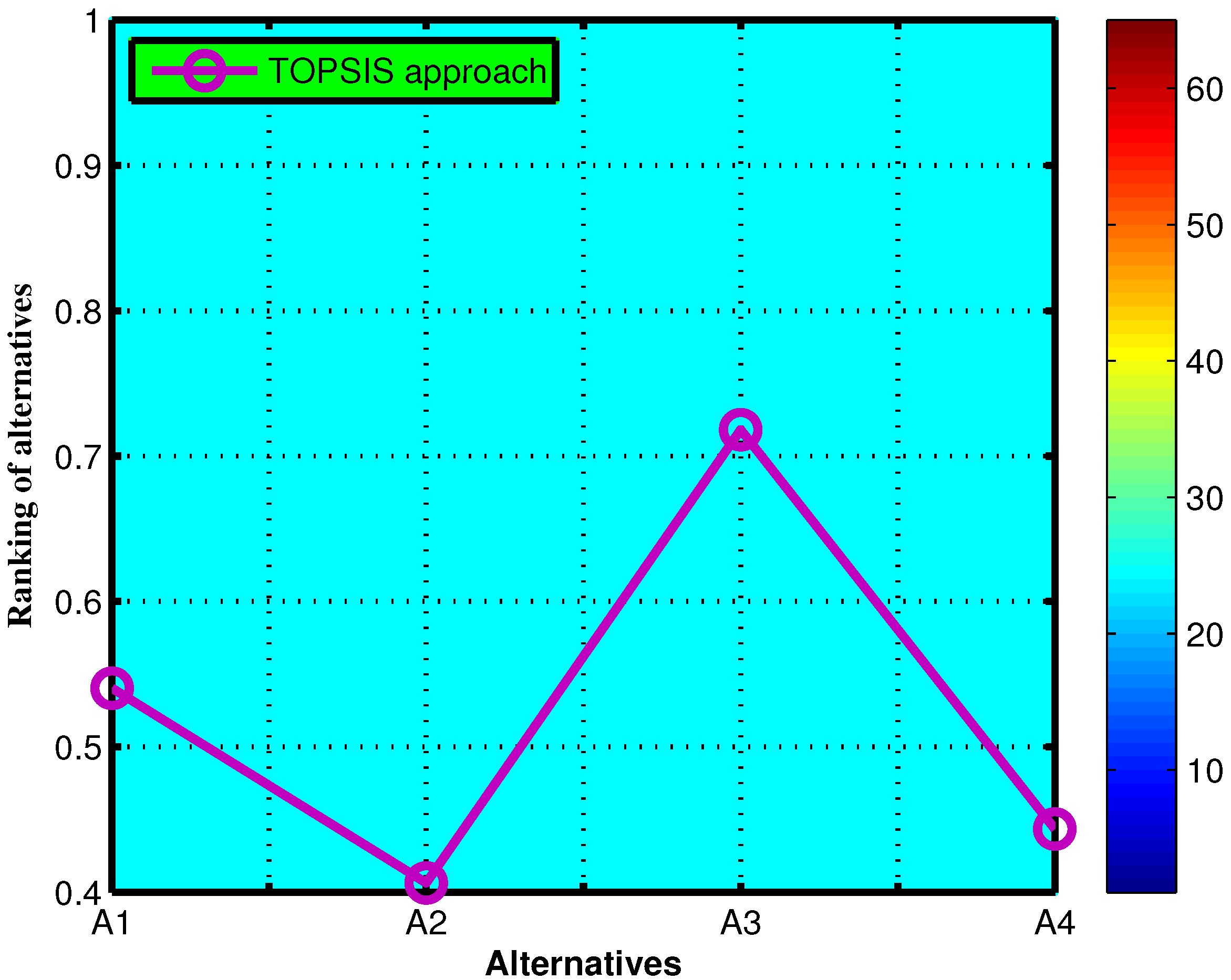
The relative closeness indices for each DMs of the alternatives. 0.5403 0.4064 0.7182 0.4436 - Step-7
- The alternatives are ranked in descending order, as presented in Table 16. The minimum distance can be observed in . Therefore, based on the given information, it can be determined that is the most suitable selection among the alternatives. The geometrical representation of ranking order using the TOPSIS approach is illustrated in Figure 4.
Table 16. Ranking order of alternatives.
 Figure 4. Geometrical portrayal of ranking order using TOPSIS approach.
7.2. Characteristic and Analytical Comparison
In order to address challenges in the real world, the established technique may also cope with existing methods ([1,44,66,67,68,69,70]). These features enable it to be used for real-world problems. In order to demonstrate how the proposed method stacks up compared to the existing methods for multi-parameter DM, a comparison investigation was carried out utilising multiple frameworks that were developed by various researchers. Table 17 provides an analysis of the existing approach utilising IHFRSs in contrast to the traditional strategies, while Table 18 provides a comparison of characteristics. Therefore, our suggested approaches are superior to the traditional approaches.
Table 17.
Analytical comparison with existing approaches.
Table 18.
Characteristic comparison between the present approach together with conventional approaches.
8. Conclusions and Future Recommendations
The significant contribution of this article is the introduction of the novel notion of intuitionistic hesitant fuzzy rough sets and their set theoretical operations. We introduced novel operational rules for IHFR numbers based on Dombi t-norm and Dombi t-conorm operations. Furthermore, we listed a list of new information aggregation operators based on the aforementioned operating laws, including IHFRDWA, IHFRDOWA, and IHFRDHWA aggregation operators. The essential attributes of the developed operators are investigated. Moreover, we developed an MADM methodology and demonstrated their application to the MADM problem of choosing a suitable worldwide partnership. The sensitivity analysis is addressed, and the findings were examined for various parameters for the ranking order, and it was determined that raising the parameter value seemed to have no influence on the ranking order. To validate the findings, an improved TOPSIS-technique-based IHFRS is carried out and the outcomes are compared to those obtained by the suggested operators. This reiterates the reliability and dependability of the presented approach, which may be used for worldwide challenging decision-making challenges. In the future, our research will be oriented on the establishment of aggregation operators for a probabilistic uncertain linguistic term set [72,73,74,75], ELICIT information [76], and consensus reaching processes [77,78,79,80,81,82,83,84]. We will further enhance the notation for different aggregation operators, similarity and distance measures, and decision-making techniques based on TODIM, TAOV, and VIKOR. In addition, we plan to implement multiple support tools for multi-criteria decision analysis (MCDA), such as the characteristic objects method (COMET), expected solution point COMET, stable preference ordering towards the ideal solution (SPOTIS), and reference ideal method (RIM). Furthermore, we will present a new sensitivity analysis method called the comprehensive sensitivity analysis method (COMSAM) in our upcoming research [85,86]. These methods allow for systematic modification of multiple values within the decision matrix. The aforementioned approaches will be used for the selection process in other manufacturing environments, pharmaceutical, automotive industries, and many others, such as [87,88,89].
Author Contributions
Conceptualization, A. and S.A.; methodology, A., S.A. and Y.A.; software, A.; validation, A., S.A. and M.A.; formal analysis, A. and Y.A.; investigation, A. and M.A.; resources, A. and M.A.; data curation, A.; writing—original draft preparation, A. and S.A.; writing—review and editing, A.; visualization, A., M.A. and Y.A.; supervision, A. and S.A.; project administration, A. and S.A.; funding acquisition, S.A., M.A. and Y.A. All authors have read and agreed to the published version of the manuscript.
Funding
The APC was funded by Sultan Alyobi.
Institutional Review Board Statement
This article does not contain any studies with human participants or animals performed by any of the authors.
Data Availability Statement
All the data are available in the manuscript.
Acknowledgments
The authors are thankful to the Deanship of Graduate Studies and Scientific Research at University of Bisha for supporting this work through the Fast-Track Research Support Program.
Conflicts of Interest
All the authors declare that they have no known competing financial interests or personal relationships that could have appeared to influence the work reported in this paper.
Appendix A
Proof of Theorem 1.
Proof.
The theorem can be proven by employing the mathematical induction approach.
- When , we obtain the following findings based on Dombi operations as
- Suppose the result is true for ; that is,whenSo, the result is true for all Hence, the theorem is proven for all
□
References
- Zadeh, L. Fuzzy sets. Inf. Control 1965, 8, 338–353. [Google Scholar] [CrossRef]
- Atanassov, K. Intuitionistic fuzzy sets. Int. J. Bioautomation 2016, 20, 1. [Google Scholar]
- Yager, R.R. Pythagorean fuzzy subsets. In Proceedings of the 2013 Joint IFSA World Congress and NAFIPS Annual Meeting (IFSA/NAFIPS), Edmonton, AB, Canada, 24–28 June 2013; pp. 57–61. [Google Scholar]
- Pawlak, Z. Rough sets. Int. J. Comput. Inf. Sci. 1982, 11, 341–356. [Google Scholar] [CrossRef]
- Li, T.; Nguyen, H.S.; Wang, G.; Grzymala-Busse, J.W.; Janicki, R.; Hassanien, A.E.; Yu, H. Rough Sets and Knowledge Technology; Springer: Berlin/Heidelberg, Germany, 2012. [Google Scholar]
- Pawlak, Z. Rough sets and intelligent data analysis. Inf. Sci. 2002, 147, 1–12. [Google Scholar] [CrossRef]
- Dubois, D.; Prade, H. Rough fuzzy sets and fuzzy rough sets. Int. J. Gen. Syst. 1990, 17, 191–209. [Google Scholar] [CrossRef]
- Cornelis, C.; DeCock, M.; Kerre, E.E. Intuitionistic fuzzy rough sets: At the crossroads of imperfect knowledge. Expert Syst. 2003, 20, 260–270. [Google Scholar] [CrossRef]
- Samanta, S.; Mondal, T. Intuitionistic fuzzy rough sets and rough intuitionistic fuzzy sets. J. Fuzzy Math. 2001, 9, 561–582. [Google Scholar]
- Zhou, L.; Wu, W.-Z. On generalized intuitionistic fuzzy rough approximation operators. Inf. Sci. 2008, 178, 2448–2465. [Google Scholar] [CrossRef]
- Huang, B.; Li, H.; Wei, D. Dominance-based rough set model in intuitionistic fuzzy information systems. Knowl.-Based Syst. 2012, 28, 115–123. [Google Scholar] [CrossRef]
- Huang, B.; Wei, D.; Li, H.; Zhuang, Y. Using a rough set model to extract rules in dominance-based interval-valued intuitionistic fuzzy information systems. Inf. Sci. 2013, 221, 215–229. [Google Scholar] [CrossRef]
- Zhou, L.; Wu, W.-Z.; Zhang, W.-X. On characterization of intuitionistic fuzzy rough sets based on intuitionistic fuzzy implicators. Inf. Sci. 2009, 179, 883–898. [Google Scholar] [CrossRef]
- Feng, F.; Li, C.; Davvaz, B.; Ali, M.I. Soft sets combined with fuzzy sets and rough sets: A tentative approach. Soft Comput. 2010, 14, 899–911. [Google Scholar] [CrossRef]
- Feng, F.; Liu, X.; Leoreanu-Fotea, V.; Jun, Y.B. Soft sets and soft rough sets. Inf. Sci. 2011, 181, 1125–1137. [Google Scholar] [CrossRef]
- Shabir, M.; Ali, M.I.; Shaheen, T. Another approach to soft rough sets. Knowl.-Based Syst. 2013, 40, 72–80. [Google Scholar] [CrossRef]
- Sun, B.; Ma, W. Soft fuzzy rough sets and its application in decision making. Artif. Intell. Rev. 2014, 41, 67–80. [Google Scholar] [CrossRef]
- Zhang, Z. Generalized intuitionistic fuzzy rough sets based on intuitionistic fuzzy coverings. Inf. Sci. 2012, 198, 186–206. [Google Scholar] [CrossRef]
- Hussain, A.; Ali, M.I.; Mahmood, T. Pythagorean fuzzy soft rough sets and their applications in decision-making. J. Taibah Univ. Sci. 2020, 14, 101–113. [Google Scholar] [CrossRef]
- Hussain, A.; IrfanAli, M.; Mahmood, T. Covering based q-rung orthopair fuzzy rough set model hybrid with topsis for multi-attribute decision making. J. Intell. Fuzzy Syst. 2019, 37, 981–993. [Google Scholar] [CrossRef]
- Hussain, A.; Mahmood, T.; Ali, M.I. Rough pythagorean fuzzy ideals in semigroups. Comput. Appl. Math. 2019, 38, 1–15. [Google Scholar] [CrossRef]
- Wan, S.-P.; Yi, Z.-H. Power average of trapezoidal intuitionistic fuzzy numbers using strict t-norms and t-conorms. IEEE Trans. Fuzzy Syst. 2015, 24, 1035–1047. [Google Scholar] [CrossRef]
- Wan, S.-P.; Wang, F.; Lin, L.-L.; Dong, J.-Y. Some new generalized aggregation operators for triangular intuitionistic fuzzy numbers and application to multi-attribute group decision making. Comput. Ind. Eng. 2016, 93, 286–301. [Google Scholar] [CrossRef]
- Ahmmad, J.; Mahmood, T.; Mehmood, N.; Urawong, K.; Chinram, R. Intuitionistic fuzzy rough aczel-alsina average aggregation operators and their applications in medical diagnoses. Symmetry 2022, 14, 2537. [Google Scholar] [CrossRef]
- Zheng, L.; Mahmood, T.; Ahmmad, J.; Rehman, U.U.; Zeng, S. Spherical fuzzy soft rough average aggregation operators and their applications to multi-criteria decision making. IEEE Access 2022, 10, 27832–27852. [Google Scholar] [CrossRef]
- Cornelis, C.; Verbiest, N.; Jensen, R. Ordered weighted average based fuzzy rough sets. In Rough Set and Knowledge Technology; Springer: Berlin/Heidelberg, Germany, 2010; pp. 78–85. [Google Scholar]
- Liu, H.B.; Liu, Y.; Xu, L. Dombi interval-valued hesitant fuzzy aggregation operators for information security risk assessment. Math. Probl. Eng. 2020, 2020, 3198645. [Google Scholar] [CrossRef]
- Akram, M.; Yaqoob, N.; Ali, G.; Chammam, W. Extensions of dombi aggregation operators for decision making under m-polar fuzzy information. J. Math. 2020, 2020, 4739567. [Google Scholar] [CrossRef]
- Tehreem; Hussain, A.; Alsanad, A. Novel dombi aggregation operators in spherical cubic fuzzy information with applications in multiple attribute decision-making. Math. Probl. Eng. 2021, 2021, 9921553. [Google Scholar]
- Ashraf, S.; Abdullah, S.; Mahmood, T. Spherical fuzzy dombi aggregation operators and their application in group decision making problems. J. Ambient Intell. Humaniz. Comput. 2020, 11, 2731–2749. [Google Scholar] [CrossRef]
- Chen, J.; Ye, J. Some single-valued neutrosophic dombi weighted aggregation operators for multiple attribute decision-making. Symmetry 2017, 9, 82. [Google Scholar] [CrossRef]
- Shi, L.; Ye, J. Dombi aggregation operators of neutrosophic cubic sets for multiple attribute decision-making. Algorithms 2018, 11, 29. [Google Scholar] [CrossRef]
- Lu, X.; Ye, J. Dombi aggregation operators of linguistic cubic variables for multiple attribute decision making. Information 2018, 9, 188. [Google Scholar] [CrossRef]
- He, X. Typhoon disaster assessment based on dombi hesitant fuzzy information aggregation operators. Nat. Hazards 2018, 90, 1153–1175. [Google Scholar] [CrossRef]
- Jana, C.; Senapati, T.; Pal, M.; Yager, R.R. Picture fuzzy Dombi aggregation operators: Application to MADM process. Appl. Soft Comput. 2019, 74, 99–109. [Google Scholar] [CrossRef]
- Hwang, C.-L.; Masud, A.S.M. Multiple Objective Decision Making Methods and Applications: A State-of-the-Art Survey; Springer: Berlin/Heidelberg, Germany, 2012; Volume 164. [Google Scholar]
- Umer, R.; Touqeer, M.; Omar, A.H.; Ahmadian, A.; Salahshour, S.; Ferrara, M. Selection of solar tracking system using extended topsis technique with interval type-2 pythagorean fuzzy numbers. Optim. Eng. 2021, 22, 2205–2231. [Google Scholar] [CrossRef]
- Pishyar, S.; Khosravi, H.; Tavili, A.; Malekian, A.; Sabourirad, S. A combined ahp-and topsis-based approach in the assessment of desertification disaster risk. Environ. Model. Assess. 2020, 25, 219–229. [Google Scholar] [CrossRef]
- Kacprzak, D. An extended topsis method based on ordered fuzzy numbers for group decision making. Artif. Intell. Rev. 2020, 53, 2099–2129. [Google Scholar] [CrossRef]
- Rani, P.; Mishra, A.R.; Rezaei, G.; Liao, H.; Mardani, A. Extended pythagorean fuzzy topsis method based on similarity measure for sustainable recycling partner selection. Int. J. Fuzzy Syst. 2020, 22, 735–747. [Google Scholar] [CrossRef]
- Jun, H.; Junmin, W.; Jie, W. Topsis hybrid multiattribute group decision-making based on interval pythagorean fuzzy numbers. Math. Probl. Eng. 2021, 2021, 5735272. [Google Scholar] [CrossRef]
- Zhao, H.; Xu, Z.; Ni, M.; Cui, F. Hybrid fuzzy multiple attribute decision making. Inf. Int. Interdiscip. J. 2009, 12, 1033–1044. [Google Scholar]
- Zhang, K.; Dai, J. A novel topsis method with decision-theoretic rough fuzzy sets. Inf. Sci. 2022, 608, 1221–1244. [Google Scholar] [CrossRef]
- Torra, V. Hesitant fuzzy sets. Int. J. Intell. Syst. 2010, 25, 529–539. [Google Scholar] [CrossRef]
- Liao, H.; Xu, Z.; Xia, M. Multiplicative consistency of hesitant fuzzy preference relation and its application in group decision making. Int. J. Inf. Technol. Decis. Mak. 2014, 13, 47–76. [Google Scholar] [CrossRef]
- Ebrahimpour, M.K.; Eftekhari, M. Ensemble of feature selection methods: A hesitant fuzzy sets approach. Appl. Soft Comput. 2017, 50, 300–312. [Google Scholar] [CrossRef]
- Sun, G.; Guan, X.; Yi, X.; Zhou, Z. Grey relational analysis between hesitant fuzzy sets with applications to pattern recognition. Expert Syst. Appl. 2018, 92, 521–532. [Google Scholar] [CrossRef]
- Xu, Z.; Zhang, X. Hesitant fuzzy multi-attribute decision making based on topsis with incomplete weight information. Knowl.-Based Syst. 2013, 52, 53–64. [Google Scholar] [CrossRef]
- Feng, X.; Tan, Q.; Wei, C. Hesitant fuzzy linguistic multi-criteria decision making based on possibility theory. Int. J. Mach. Learn. Cybern. 2018, 9, 1505–1517. [Google Scholar] [CrossRef]
- Qian, Y.; Liang, J.; Yao, Y.; Dang, C. Mgrs: A multi-granulation rough set. Inf. Sci. 2010, 180, 949–970. [Google Scholar] [CrossRef]
- Qian, Y.; Liang, X.; Wang, Q.; Liang, J.; Liu, B.; Skowron, A.; Yao, Y.; Ma, J.; Dang, C. Local rough set: A solution to rough data analysis in big data. Int. J. Approx. Reason. 2018, 97, 38–63. [Google Scholar] [CrossRef]
- Yang, X.; Song, X.; Qi, Y.; Yang, J. Constructive and axiomatic approaches to hesitant fuzzy rough set. Soft Comput. 2014, 18, 1067–1077. [Google Scholar] [CrossRef]
- Zhang, H.; Shu, L.; Liao, S. Hesitant fuzzy rough set over two universes and its application in decision making. Soft Comput. 2017, 21, 1803–1816. [Google Scholar] [CrossRef]
- Torra, V.; Narukawa, Y. On hesitant fuzzy sets and decision. In Proceedings of the 2009 IEEE International Conference on Fuzzy Systems, Jeju, Republic of Korea, 20–24 August 2009; pp. 1378–1382. [Google Scholar]
- Beg, I.; Rashid, T. Group decision making using intuitionistic hesitant fuzzy sets. Int. J. Fuzzy Log. Intell. Syst. 2014, 14, 181–187. [Google Scholar] [CrossRef]
- Chinram, R.; Hussain, A.; Mahmood, T.; Ali, M.I. Edas method for multi-criteria group decision making based on intuitionistic fuzzy rough aggregation operators. IEEE Access 2021, 9, 10199–10216. [Google Scholar] [CrossRef]
- Dombi, J. A general class of fuzzy operators, the demorgan class of fuzzy operators and fuzziness measures induced by fuzzy operators. Fuzzy Sets Syst. 1982, 8, 149–163. [Google Scholar] [CrossRef]
- Hsu, P.-F.; Hsu, M.-G. Optimizing the information outsourcing practices of primary care medical organizations using entropy and topsis. Qual. Quant. 2008, 42, 181–201. [Google Scholar] [CrossRef]
- Tzeng, G.-H.; Huang, J.-J. Multiple Attribute Decision Making: Methods and Applications; CRC Press: Boca Raton, FL, USA, 2011. [Google Scholar]
- Yu, C.; Shao, Y.; Wang, K.; Zhang, L. A group decision making sustainable supplier selection approach using extended topsis under interval-valued pythagorean fuzzy environment. Expert Syst. Appl. 2019, 121, 1–17. [Google Scholar] [CrossRef]
- Chakraborty, S. Applications of the moora method for decision making in manufacturing environment. Int. J. Adv. Manuf. Technol. 2011, 54, 1155–1166. [Google Scholar] [CrossRef]
- Bolturk, E.; Kahraman, C. A novel interval-valued neutrosophic ahp with cosine similarity measure. Soft Comput. 2018, 22, 4941–4958. [Google Scholar] [CrossRef]
- Mir, M.A.; Ghazvinei, P.T.; Sulaiman, N.; Basri, N.; Saheri, S.; Mahmood, N.; Jahan, A.; Begum, R.; Aghamohammadi, N. Application of topsis and vikor improved versions in a multi criteria decision analysis to develop an optimized municipal solid waste management model. J. Environ. Manag. 2016, 166, 109–115. [Google Scholar]
- Akram, M.; Shumaiza; Arshad, M. Bipolar fuzzy topsis and bipolar fuzzy electre-i methods to diagnosis. Comput. Appl. Math. 2020, 39, 1–21. [Google Scholar] [CrossRef]
- Behzadian, M.; Kazemzadeh, R.B.; Albadvi, A.; Aghdasi, M. Promethee: A comprehensive literature review on methodologies and applications. Eur. J. Oper. Res. 2010, 200, 198–215. [Google Scholar] [CrossRef]
- Akram, M.; Adeel, A.; Alcantud, J.C.R. Group decision-making methods based on hesitant n-soft sets. Expert Syst. Appl. 2019, 115, 95–105. [Google Scholar] [CrossRef]
- Akram, M.; Adeel, A.; Alcantud, J.C.R. Hesitant fuzzy n-soft sets: A new model with applications in decision-making. J. Intell. Fuzzy Syst. 2019, 36, 6113–6127. [Google Scholar] [CrossRef]
- Ashraf, S.; Kousar, M.; Hameed, M.S. Early infectious diseases identification based on complex probabilistic hesitant fuzzy n-soft information. Soft Comput. 2023, 27, 18285–18310. [Google Scholar] [CrossRef] [PubMed]
- Garg, H.; Mahmood, T.; Rehman, U.; Ali, Z. Chfs: Complex hesitant fuzzy sets-their applications to decision making with different and innovative distance measures. CAAI Trans. Intell. Technol. 2021, 6, 93–122. [Google Scholar] [CrossRef]
- Zhang, S.; Xu, Z.; He, Y. Operations and integrations of probabilistic hesitant fuzzy information in decision making. Inf. Fusion 2017, 38, 1–11. [Google Scholar] [CrossRef]
- Mahmood, T.; UrRehman, U.; Ali, Z. A novel complex fuzzy n-soft sets and their decision-making algorithm. Complex Intell. Syst. 2021, 7, 2255–2280. [Google Scholar] [CrossRef]
- Saha, A.; Senapati, T. Yager, R.R. Hybridizations of generalized dombi operators and bonferroni mean operators under dual probabilistic linguistic environment for group decision-making. Int. J. Intell. Syst. 2021, 36, 6645–6679. [Google Scholar] [CrossRef]
- Su, Y.; Zhao, M.; Wei, G.; Wei, C.; Chen, X. Probabilistic uncertain linguistic edas method based on prospect theory for multiple attribute group decision-making and its application to green finance. Int. J. Fuzzy Syst. 2022, 24, 1318–1331. [Google Scholar] [CrossRef]
- Wei, G.; Lin, R.; Lu, J.; Wu, J.; Wei, C. The generalized dice similarity measures for probabilistic uncertain linguistic magdm and its application to location planning of electric vehicle charging stations. Int. J. Fuzzy Syst. 2022, 24, 933–948. [Google Scholar] [CrossRef]
- Zhao, M.; Wei, G.; Wei, C.; Wu, J. Pythagorean fuzzy todim method based on the cumulative prospect theory for magdm and its application on risk assessment of science and technology projects. Int. J. Fuzzy Syst. 2021, 23, 1027–1041. [Google Scholar] [CrossRef]
- Romero, Á.L.; Rodríguez, R.M.; Martínez, L. Computing with comparative linguistic expressions and symbolic translation for decision making: Elicit information. IEEE Trans. Fuzzy Syst. 2019, 28, 2510–2522. [Google Scholar] [CrossRef]
- García-Zamora, D.; Labella, Á.; Ding, W.; Rodríguez, R.M.; Martínez, L. Large-scale group decision making: A systematic review and a critical analysis. IEEE/CAA J. Autom. Sin. 2022, 9, 949–966. [Google Scholar] [CrossRef]
- Labella, Á.; Liu, H.; Rodríguez, R.M.; Martínez, L. A cost consensus metric for consensus reaching processes based on a comprehensive minimum cost model. Eur. J. Oper. Res. 2020, 281, 316–331. [Google Scholar] [CrossRef]
- Labella, Á.; Liu, Y.; Rodríguez, R.; Martínez, L. Analyzing the performance of classical consensus models in large scale group decision making: A comparative study. Appl. Soft Comput. 2018, 67, 677–690. [Google Scholar] [CrossRef]
- Lei, W.; Ma, W.; Li, X.; Sun, B. Three-way group decision based on regret theory under dual hesitant fuzzy environment: An application in water supply alternatives selection. Expert Syst. Appl. 2024, 237, 121249. [Google Scholar] [CrossRef]
- Ransikarbum, K.; Pitakaso, R. Multi-objective optimization design of sustainable biofuel network with integrated fuzzy analytic hierarchy process. Expert Syst. Appl. 2024, 240, 122586. [Google Scholar] [CrossRef]
- Rodríguez, R.M.; Labella, Á.; DeTré, G.; Martínez, L. A large scale consensus reaching process managing group hesitation. Knowl.-Based Syst. 2018, 159, 86–97. [Google Scholar] [CrossRef]
- Xu, L.; Hu, X.; Zhang, Y.; Feng, J.; Luo, S. A fuzzy multiobjective team decision model for codp and supplier selection in customized logistics service supply chain. Expert Syst. Appl. 2024, 237, 121387. [Google Scholar] [CrossRef]
- Zhou, X.; Tan, W.; Sun, Y.; Huang, T.; Yang, C. Multi-objective optimization and decision making for integrated energy system using sta and fuzzy topsis. Expert Syst. Appl. 2024, 240, 122539. [Google Scholar] [CrossRef]
- Shekhovtsov, A.; Kizielewicz, B.; Salabun, W. Advancing individual decision-making: An extension of the characteristic objects method using expected solution point. Inf. Sci. 2023, 647, 119456. [Google Scholar] [CrossRef]
- Wieckowski, J.; Salabun, W. A new sensitivity analysis method for decision-making with multiple parameters modification. Inf. Sci. 2024, 678, 120902. [Google Scholar] [CrossRef]
- Antczak, T. On optimality for fuzzy optimization problems with granular differentiable fuzzy objective functions. Expert Syst. Appl. 2024, 240, 121891. [Google Scholar] [CrossRef]
- Song, H.-H.; Dutta, B.; García-Zamora, D.; Wang, Y.-M.; Martínez, L. Managing non-cooperative behaviors in consensus reaching process: A novel multi-stage linguistic lsgdm framework. Expert Syst. Appl. 2024, 240, 122555. [Google Scholar] [CrossRef]
- Wu, M.; Song, J.; Fan, J. A q-rung orthopair fuzzy multi-attribute group decision making model based on attribute reduction and evidential reasoning methodology. Expert Syst. Appl. 2024, 240, 122558. [Google Scholar] [CrossRef]


Disclaimer/Publisher’s Note: The statements, opinions and data contained in all publications are solely those of the individual author(s) and contributor(s) and not of MDPI and/or the editor(s). MDPI and/or the editor(s) disclaim responsibility for any injury to people or property resulting from any ideas, methods, instructions or products referred to in the content. |
© 2024 by the authors. Licensee MDPI, Basel, Switzerland. This article is an open access article distributed under the terms and conditions of the Creative Commons Attribution (CC BY) license (https://creativecommons.org/licenses/by/4.0/).