Multi-Attribute Decision-Making Based on Consistent Bidirectional Projection Measures of Triangular Dual Hesitant Fuzzy Set

Abstract

To solve complex multi-attribute decision-making (MADM) problems within a triangular dual hesitant fuzzy (TDHF) environment where the attribute weights (Aws) are either fully or partially known, a novel bidirectional projection method is proposed, named multi-attribute decision-making and based on the consistent bidirectional projection measures of triangular dual hesitant fuzzy sets (TDHFSs). First, some notions are developed, such as the operation laws, score and accuracy functions, negative ideal points (NIPs), and positive ideal points (PIPs) of TDHFSs. The correlation coefficients and the cosine of the angle between the vectors of each alternative and the triangular dual hesitant fuzzy (TDHF) points are introduced. Then, the consistent bidirectional projection decision-making method based on the TDHFSs’ correlation coefficients is proposed. Additionally, an optimization model is established via maximizing the consistent coefficient to determine the Aws. Furthermore, some approaches are investigated based on the proposed approaches concerning the MADM issues with attribute values represented by triangular dual hesitant fuzzy elements (TDHFEs). Finally, a supply chain management (SCM) problem is illustrated, and comparative analyses are implemented to demonstrate the presented approach’s feasibility and efficiency.

1. Introduction

Since the decision-making environment is complex and decision-makers (DMs) have limited knowledge, dealing with decision-making issues using crisp values is challenging. To address this issue, Zadeh [1] presented fuzzy sets (FSs) in 1965, providing a significant convenience for dealing with fuzzy and vague information. Subsequently, scholars have paid more attention to fuzzy theories and expanded FSs in other directions, including type-2 fuzzy [2], intuitionistic fuzzy [3,4], vague [5,6], neutrosophic [7], and Pythagorean fuzzy sets (PFSs) [8,9].

Hesitant fuzzy sets (HFSs) were put forward by Torra [10,11], allowing membership with a set of possible values, making them an effective generalization of traditional fuzzy sets (FSs). Farhadinia [12,13] later proposed a series of measurement tools for HFSs and interval-valued hesitant fuzzy sets (IVHFSs). Xia et al. [14] introduced hesitant fuzzy element (HFE) operational laws and developed various hesitant fuzzy operators. Xu et al. [15] defined the distance and correlation metrics and proved some desirable features of HFEs. Peng et al. [16] and Xu et al. [17] discussed various measurement techniques for HFSs. Xu et al. [18] and Zhang et al. [19] presented TOPSIS and TOMID decision-making approaches in hesitant fuzzy environments. He et al. [20] introduced the hesitant fuzzy geometric Bonferroni mean (HFGBM) and hesitant fuzzy Choquet geometric Bonferroni mean (HFCGBM) operators.

Additionally, Chen et al. [21] presented the idea of IVHFSs to meet actual decision-making environment requirements, allowing the membership to contain some possible interval values. They also presented the IVHFWA weighted averaging operator. Wei et al. [22] introduced the IVHFSs’ operational laws and score functions. Based on the above analysis, Zhu et al. [23] proposed dual hesitant fuzzy sets (DHFSs) and found that these include fuzzy, intuitionistic, hesitant fuzzy sets, and fuzzy multisets as particular sets. Ju et al. [24] investigated IVDHFSs and developed various operators to combine IVDHF information. Zang et al. [25] proposed the IVDHF Heronian mean operators, which can solve interactive MADM issues. Su et al. [26] presented some distance and similarity metrics for IVDHFSs.

In real decision-making problems, triangular fuzzy values are more suitable for dealing with fuzzy and imprecise information than the crisp and interval values in human judgments. However, under many conditions, for real multiple-attribute group decision-making problems, the decision information about alternatives is usually uncertain or fuzzy due to the increasing complexity of the socio-economic environment and the vagueness of the inherent subjective nature of human thinking, thus, exact and crisp values are inadequate or insufficient to model real-life decision-making problems. Indeed, human judgments including preference information may be stated, which permits the membership to have a set of possible triangular fuzzy values. On the other hand, in practical applications, using interval numbers to represent evaluation information can lead to challenges. If the interval is too large, it may contain excessive irrelevant information; if too small, critical details may be lost, resulting in incomplete information. In contrast, triangular fuzzy numbers offer distinct advantages: (1) their membership functions assign higher membership values to central points and lower membership values to boundary points, minimizing the impact of boundary values on the quantitative description of information; (2) additionally, triangular fuzzy numbers more closely align with human cognitive processes compared to interval fuzzy numbers.

Given these advantages, the current paper presents the new idea of triangular dual hesitant fuzzy sets (TDHFSs), where two sets of possible triangular values describe the membership degree (MD) and non-membership degree (NMD) of an element for a defined set. TDHFSs can be seen as more collective sets; that is, the MD- and NMD-based functions support this further flexibility and effective method as DMs give their corresponding opinions. In this case, we also must deal with two hesitancies. Furthermore, the traditional sets involving FSs, IFSs, and HFSs can be considered particular types of TDHFSs, and we do not face the triangular possibilities as in the TFSs of THFSs.

However, various possible triangular values describe whether the epistemic degrees are certain or uncertain. For instance, in a multi-attribute decision-making problem, DMs might consider the following possible values for the membership degrees of x into set A: (0.1, 0.2, 0.3), (0.2, 0.3, 0.4), and (0.4, 0.5, 0.6). Similarly, the non-membership degrees might include (0.5, 0.6, 0.7) and (0.6, 0.7, 0.8). Consequently, the levels of certainty and uncertainty regarding these values are not constrained, allowing decision-makers’ original information to be reflected as accurately as possible. By utilizing triangular dual hesitant fuzzy sets (TDHFSs), a broader range of information can be incorporated, and the more values we obtain from the decision-makers.

The distance measure method is always the focus of multiple-attribute decision-making (MADM), with approaches such as TOPSIS [18], VIKOR [27,28], QUALIFLEX [29], and the projection method [30] being widely used. The projection method has been widely utilized in decision-making fields because it does not require direct comparison or ranking of evaluation information and offers a high degree of differentiation; however, traditional projection methods [31,32] only consider the projection magnitude of the alternatives on the positive ideal points (PIPs) and ignore the projection magnitude on the negative ideal points (NIPs). Since this is counterintuitive, Liu [33] proposed the bidirectional projection method to overcome this shortcoming, which considers both the distance and the involved angle as well as the bidirectional projection between the PIPs and NIPs. Furthermore, Ye et al. [34] generalized the bidirectional projection approach to the neutrosophic information environment. Liu et al. [35] combined the power average operator and bidirectional projection approach and extended fusion operators to the probabilistic linguistic information environment. Liu et al. [36] developed a bidirectional projection method with linguistic neutrosophic sets (LNSs).

Up until now, the bidirectional projection method employed for dealing with uncertain problems has attained some developments in theoretical areas. Thus, the bidirectional projection approach should be generalized to handle triangular hesitant fuzzy problems in this paper. The essential novelties and contributions of this work can be described as the following:

• This paper introduces triangular dual hesitant fuzzy sets (TDHFSs) and establishes the basic operational rules. This allows the dual relationship between membership and non-membership degrees to be used in identifying objects with unclear boundaries;
• A consistent bidirectional projection method is proposed. Unlike existing methods, the consistent bidirectional projection method measures the relative closeness of alternatives to the positive and negative ideal points rather than relying solely on absolute numerical differences, thereby minimizing information loss. The presented method has higher discrimination and sensitivity;
• The consistent bidirectional projection method is further extended to handle triangular dual hesitant fuzzy information. It not only accounts for the projection distance, the included angle, and the consistent relationship between positive and negative ideal points but also considers membership degree and non-membership degree.

The remainder of this manuscript is organized as follows. The essential ideas of DHFSs and IVDHFSs and some operation laws operation are described briefly in Section 2. The new concept of TDHFSs is presented and some of its essential operations and features are verified. In Section 3, the consistent bidirectional projection and the optimization model are constructed. In Section 4, the proposed consistent bidirectional projection approach is applied, using the maximizing consistency coefficient to obtain attribute weights (Aws). Section 5 discusses the proposed consistent bidirectional projection approach based on TDHFSs and demonstrates the superiority of the presented approach through a comparative analysis. Finally, the manuscript concludes the research and provides future directions.

2. Preliminary Methods

2.1. Dual Hesitant Fuzzy Elements

Definition 1 

([14]). Let $X$ be a non-empty fixed set. The HFS $H$ on $X$ is described as a mapping ${\tilde{h}}_H(x)$ returning a subset of $[0,1]$ after applying to $X$. H describes the HFS as follows:

$$H=\left\{\langle x,{\tilde{h}}_H(x)\rangle |x\in X\right\},$$

(1)

where ${\tilde{h}}_H(x)$ describes a set of some distinct scores in $[0,1]$ describing the MDs of $x\in X$ to $H$ . For the sake of simplicity, $\tilde{h}={\tilde{h}}_H(x)$ is defined as an HFE, the basic unit of HFSs.

Definition 2 

([23]). Consider that $X$ is a non-empty fixed set. The DHFS $H$ on $X$ can be described as

$$D=\left\{〈x,\right.\left.h(x),g(x)〉\right|\left.x\in X\right\},$$

(2)

where $h(x)$ and $g(x)$ describe two sets of some distinct scores in $[0,1]$, indicating the possible MDs and NMDs of $x\in X$to $D$ with the following conditions—$\gamma ,\eta \in [0,1],$ $0\le {\gamma }^{+}+{\eta }^{+}\le 1,$ where $\gamma \in h(x),$ $\eta \in g(x),$ ${\gamma }^{+}\in h^{+}(x)={\cup }_{\gamma \in h(x)}\max \left\{\gamma \right\}$, and ${\eta }^{+}\in g^{+}(x)$ $={\cup }_{\eta \in g(x)}\max \left\{\eta \right\}$ for any $x\in X$. The pair $d(x)=\left\{h(x),g(x)\right\}$ is a DHF element (DHFE), described by $\tilde{d}=\left\{\tilde{h},\tilde{g}\right\}$.

Definition 3 

([23]). Consider that $d=(h,g)$,$d_1=(h_1,g_1)$, and $d_2=(h_2,g_2)$ are three DHFEs, where their basic operational rules are described by $\lambda >0$:

(1) 

$d^{\lambda }={\cup }_{\gamma \in h,\eta \in g}\left\{({\gamma }^{\lambda }),(1-{(1-\eta )}^{\lambda })\right\}$ ;

(2) 

$\lambda d={\cup }_{\gamma \in h,\eta \in g}\left\{(1-{(1-\gamma )}^{\lambda }),({\eta }^{\lambda })\right\}$ ;

(3) 

$d_1\oplus d_2={\cup }_{{\gamma }_1\in h_1,{\gamma }_2\in h_2,{\eta }_1\in g_1,{\eta }_2\in g_2}\left\{({\gamma }_1+{\gamma }_2-{\gamma }_1{\gamma }_2),({\eta }_1{\eta }_2)\right\}$ ;

(4) 

$d_1\otimes d_2={\cup }_{{\gamma }_1\in h_1,{\gamma }_2\in h_2,{\eta }_1\in g_1,{\eta }_2\in g_2}\left\{({\gamma }_1{\gamma }_2),({\eta }_1+{\eta }_2-{\eta }_1{\eta }_2)\right\}$.

2.2. Inter-Valued Dual Hesitant Fuzzy Sets

Definition 4 

([24]). Consider that $X$ is a non-empty fixed set. The IVDHFS $\tilde{D}$ on $X$ is described by $\tilde{D}=\left\{〈x,\right.\left.\tilde{h}(x),\tilde{g}(x)〉\right|\left.x\in X\right\},$ where $\tilde{h}(x)={\cup }_{[{\gamma }^l,{\gamma }^u]\in \tilde{h}(x)}\left\{[{\gamma }^l,{\gamma }^u]\right\}$ and $\tilde{g}(x)={\cup }_{[{\eta }^l,{\eta }^u]\in \tilde{g}(x)}$ $\left\{[{\eta }^l,{\eta }^u]\right\}$ describe two sets of distinct scores in $[0,1]$, indicating the possible MD and NMD of $x\in X$ to $\tilde{D}$.

This is calculated with the conditions $[{\gamma }^l,{\gamma }^u],[{\eta }^l,{\eta }^u]\in [0,1]$, $0\le {\gamma }^{u+}+{\eta }^{u+}\le 1,$ where $[{\gamma }^l,{\gamma }^u]\in \tilde{h}(x),$ $[{\eta }^l,{\eta }^u]\in \tilde{g}(x),$ ${\gamma }^{u+}\in {\tilde{h}}^{+}(x)={\cup }_{[{\gamma }^l,{\gamma }^u]\in \tilde{h}(x)}\max \left\{{\gamma }^u\right\}$, and ${\eta }^{u+}\in {\tilde{g}}^{+}(x)={\cup }_{[{\eta }^l,{\eta }^u]\in \tilde{g}(x)}$ $\max \left\{{\eta }^u\right\}$ for any $x\in X$.

The pair $\tilde{d}(x)=\left\{\tilde{h}(x),\tilde{g}(x)\right\}$ is named an IVDHFE, described as $\tilde{d}=\left\{\tilde{h},\tilde{g}\right\}$.

Definition 5 

([24]). Consider that $\tilde{d}=\left\{\tilde{h},\tilde{g}\right\}$, ${\tilde{d}}_1=\left\{{\tilde{h}}_1,{\tilde{g}}_1\right\}$, and ${\tilde{d}}_2=\left\{{\tilde{h}}_2,{\tilde{g}}_2\right\}$ are three IVDHFEs, where their operational rules are described by $\lambda >0$:

(1) 

${\tilde{d}}^{\lambda }={\cup }_{[{\gamma }^l,{\gamma }^u]\in \tilde{h}(x),[{\eta }^l,{\eta }^u]\in \tilde{g}(x)}\left\{\left\{[{({\gamma }^l)}^{\lambda },{({\gamma }^u)}^{\lambda }]\right\},\right.$ $\left.\left\{[1-{(1-{\eta }^l)}^{\lambda },1-{(1-{\eta }^u)}^{\lambda }]\right\}\right\}$;

(2) 

$\lambda \tilde{d}={\cup }_{[{\gamma }^l,{\gamma }^u]\in \tilde{h}(x),[{\eta }^l,{\eta }^u]\in \tilde{g}(x)}\left\{\left\{[1-{(1-{\gamma }^l)}^{\lambda },1-{(1-{\gamma }^u)}^{\lambda }]\right\}\right.$ $\left.\left\{[{({\eta }^l)}^{\lambda },{({\eta }^u)}^{\lambda }]\right\}\right\}$;

(3) 

${\tilde{d}}_1\oplus {\tilde{d}}_2={\cup }_{[{\gamma }^l,{\gamma }^u]\in \tilde{h}(x),[{\eta }^l,{\eta }^u]\in \tilde{g}(x)}$ $\left\{\left\{[{\gamma }_1^l+{\gamma }_2^l-{\gamma }_1^l{\gamma }_2^l,{\gamma }_1^u+{\gamma }_2^u-{\gamma }_1^u{\gamma }_2^u]\right\},\left\{[{\eta }_1^l{\eta }_2^l,{\eta }_1^u{\eta }_2^u]\right\}\right\}$;

(4) 

${\tilde{d}}_1\otimes {\tilde{d}}_2={\cup }_{[{\gamma }^l,{\gamma }^u]\in \tilde{h}(x),[{\eta }^l,{\eta }^u]\in \tilde{g}(x)}$ $\left\{\left\{[{\gamma }_1^l{\gamma }_2^l,{\gamma }_1^u{\gamma }_2^u]\right\},\left\{[{\eta }_1^l+{\eta }_2^l-{\eta }_1^l{\eta }_2^l,{\eta }_1^u+{\eta }_2^u-{\eta }_1^u{\eta }_2^u]\right\}\right\}$.

The following gives the comparison laws based on Definition 5.

Theorem 1 

([24]). Consider that $\tilde{d}=\left\{\tilde{h},\tilde{g}\right\}$, ${\tilde{d}}_1=\left\{{\tilde{h}}_1,{\tilde{g}}_1\right\}$, and ${\tilde{d}}_2=\left\{{\tilde{h}}_2,{\tilde{g}}_2\right\}$ are three IVDHFEs, where their score and accuracy functions are presented by the following:

$$S^{\prime }(\tilde{d})={\displaystyle \frac{1}{2}}\left(\begin{array}{c}{\displaystyle \frac{1}{\#\tilde{h}}}{\displaystyle {\sum }_{[{\gamma }^l,{\gamma }^u]\in \tilde{h}(x)}{\gamma }^l}-{\displaystyle \frac{1}{\#\tilde{g}}}{\displaystyle {\sum }_{[{\eta }^l,{\eta }^u]\in \tilde{g}(x)}{\eta }^l}\\ +{\displaystyle \frac{1}{\#\tilde{h}}}{\displaystyle {\sum }_{[{\gamma }^l,{\gamma }^u]\in \tilde{h}(x)}{\gamma }^u}-{\displaystyle \frac{1}{\#\tilde{g}}}{\displaystyle {\sum }_{[{\eta }^l,{\eta }^u]\in \tilde{g}(x)}{\eta }^u}\end{array}\right),$$

(3)

$$P^{\prime }(\tilde{d})={\displaystyle \frac{1}{2}}\left(\begin{array}{c}{\displaystyle \frac{1}{\#\tilde{h}}}{\displaystyle {\sum }_{[{\gamma }^l,{\gamma }^u]\in \tilde{h}(x)}{\gamma }^l}+{\displaystyle \frac{1}{\#\tilde{g}}}{\displaystyle {\sum }_{[{\eta }^l,{\eta }^u]\in \tilde{g}(x)}{\eta }^l}\\ +{\displaystyle \frac{1}{\#\tilde{h}}}{\displaystyle {\sum }_{[{\gamma }^l,{\gamma }^u]\in \tilde{h}(x)}{\gamma }^u}+{\displaystyle \frac{1}{\#\tilde{g}}}{\displaystyle {\sum }_{[{\eta }^l,{\eta }^u]\in \tilde{g}(x)}{\eta }^u}\end{array}\right).$$

(4)

where $\#h$ and $\#g$ describe the number of the elements in $\tilde{h}$ and $\tilde{g}$ , respectively.

The order relationships for ${\tilde{d}}_1$ and ${\tilde{d}}_2$ are described as the following:

(i)

If $S^{\prime }({\tilde{d}}_1)>S^{\prime }({\tilde{d}}_2)$, then ${\tilde{d}}_1\succ {\tilde{d}}_2$;

(ii)

If $S^{\prime }({\tilde{d}}_1)<S^{\prime }({\tilde{d}}_2)$, then:

(1)

If $P^{\prime }({\tilde{d}}_1)<P^{\prime }({\tilde{d}}_2)$, then ${\tilde{d}}_1\sim {\tilde{d}}_2$;

(2)

If $P^{\prime }({\tilde{d}}_1)>P^{\prime }({\tilde{d}}_2)$, then ${\tilde{d}}_1\succ {\tilde{d}}_2$.

2.3. Triangular Dual Hesitant Fuzzy Sets

In actual decision-making issues, triangular values are more suitable for dealing with fuzzy and imprecise information than crissome operational laws [37,38,39]. In this section, we introduce notions such as the definition and some operation laws of triangular dual hesitant fuzzy sets (TDHFSs).

Definition 6. 

Consider a non-empty fixed set X. The triangular dual hesitant fuzzy set (TDHFS) $\tilde{E}$ on $X$ can be described by the following:

$$\tilde{E}=\left\{\langle x,\tilde{h}(x),\tilde{g}(x)\rangle |x\in X\right\},$$

where $\tilde{h}(x)={\cup }_{({\gamma }^l,{\gamma }^m,{\gamma }^u)\in \tilde{h}(x)}\left\{({\gamma }^l,{\gamma }^m,{\gamma }^u)\right\}$ and $\tilde{g}(x)={\cup }_{({\eta }^l,{\eta }^m,{\eta }^u)\in \tilde{g}(x)}\left\{({\eta }^l,{\eta }^m,{\eta }^u)\right\}$ describe two sets of different triangular scores in $[0,1]$ , indicating the possible membership degree (MD) and non-membership degree (NMD) of $x\in X$ to $\tilde{E}$ , respectively.

This is calculated by utilizing conditions, $({\gamma }^l,{\gamma }^m,{\gamma }^u),({\eta }^l,{\eta }^m,{\eta }^u)\in [0,1]$, $0\le {\gamma }^{u+}+{\eta }^{u+}\le 1$, where $({\gamma }^l,{\gamma }^m,{\gamma }^u)\in \tilde{h}(x)$, $({\eta }^l,{\eta }^m,{\eta }^u)\in \tilde{g}(x)$, ${\gamma }^{u+}\in {\tilde{h}}^{+}(x)={\cup }_{({\gamma }^l,{\gamma }^m,{\gamma }^u)\in \tilde{h}(x)}\max \left\{{\gamma }^u\right\}$, and ${\eta }^{u+}\in {\tilde{g}}^{+}(x)={\cup }_{({\eta }^l,{\eta }^m,{\eta }^u)\in \tilde{g}(x)}\max \left\{{\eta }^u\right\}$, or all $x\in X$. The pair $\tilde{e}(x)=\left\{\tilde{h}(x),\tilde{g}(x)\right\}$ is named a TDHFE, described as $\tilde{e}=\left\{\tilde{h},\tilde{g}\right\}$.

Definition 7. 

Let $\tilde{e}=\left\{\tilde{h},\tilde{g}\right\}$, ${\tilde{e}}_1=\left\{{\tilde{h}}_1,{\tilde{g}}_1\right\}$, and ${\tilde{e}}_2=\left\{{\tilde{h}}_2,{\tilde{g}}_2\right\}$ be three TDHFEs, where their basic operational rules are defined by $\lambda >0$:

(1) 

${\tilde{e}}^{\lambda }={\cup }_{({\gamma }^l,{\gamma }^m,{\gamma }^u)\in \tilde{h}(x),({\eta }^l,{\eta }^m,{\eta }^u)\in \tilde{g}(x)}\left\{\left\{({({\gamma }^l)}^{\lambda },{({\gamma }^l)}^{\lambda },{({\gamma }^u)}^{\lambda })\right\},\right.$$\left.\left\{(1-{(1-{\eta }^l)}^{\lambda },1-{(1-{\eta }^m)}^{\lambda },1-{(1-{\eta }^u)}^{\lambda })\right\}\right\}$ ;

(2) 

$\lambda \tilde{e}={\cup }_{({\gamma }^l,{\gamma }^m,{\gamma }^u)\in \tilde{h}(x),({\eta }^l,{\eta }^m,{\eta }^u)\in \tilde{g}(x)}\left\{\left\{(1-{(1-{\gamma }^l)}^{\lambda },1-{(1-{\gamma }^m)}^{\lambda },\right.\right.$$\left.1-{(1-{\gamma }^u)}^{\lambda })\right\},\left.\left\{({({\eta }^l)}^{\lambda },{({\eta }^m)}^{\lambda },{({\eta }^u)}^{\lambda })\right\}\right\}$ ;

(3) 

${\tilde{e}}_1\oplus {\tilde{e}}_2={\cup }_{({\gamma }^l,{\gamma }^m,{\gamma }^u)\in \tilde{h}(x),({\eta }^l,{\eta }^m,{\eta }^u)\in \tilde{g}(x)}\left\{\left\{({\gamma }_1^l+{\gamma }_2^l-{\gamma }_1^l{\gamma }_2^l,\right.\right.\left.{\gamma }_1^m+{\gamma }_2^m-{\gamma }_1^m{\gamma }_2^m,{\gamma }_1^u+{\gamma }_2^u-{\gamma }_1^u{\gamma }_2^u)\right\},$ $\left.\left\{({\eta }_1^l{\eta }_2^l,{\eta }_1^m{\eta }_2^m,{\eta }_1^u{\eta }_2^u)\right\}\right\}$;

(4) 

${\tilde{e}}_1\otimes {\tilde{e}}_2={\cup }_{({\gamma }^l,{\gamma }^m,{\gamma }^u)\in \tilde{h}(x),({\eta }^l,{\eta }^m,{\eta }^u)\in \tilde{g}(x)}\left\{\left\{\left.({\gamma }_1^l{\gamma }_2^l,{\gamma }_1^m{\gamma }_2^m,{\gamma }_1^u{\gamma }_2^u)\right\}\right.\right.,\left\{({\eta }_1^l+{\eta }_2^l-{\eta }_1^l{\eta }_2^l,{\eta }_1^m+{\eta }_2^m-{\eta }_1^m{\eta }_2^m,\right.{\eta }_1^u+{\eta }_2^u$$\left.\left.-{\eta }_1^u{\eta }_2^u)\right\}\right\}$.

Thus, this work extends the concept of triangular values to the dual hesitant fuzzy (DHF) environment, introducing triangular dual hesitant fuzzy sets (TDHFSs) and establishing corresponding operational laws.

Definition 8. 

Consider a non-empty fixed set X. The TDHFS $\tilde{E}$ on $X$can be described by the following:

$$\tilde{E}=\left\{\langle x,\tilde{h}(x),\tilde{g}(x)\rangle |x\in X\right\},$$

(5)

where $\tilde{h}(x)={\cup }_{({\gamma }^l,{\gamma }^m,{\gamma }^u)\in \tilde{h}(x)}\left\{({\gamma }^l,{\gamma }^m,{\gamma }^u)\right\}$ and $\tilde{g}(x)={\cup }_{({\eta }^l,{\eta }^m,{\eta }^u)\in \tilde{g}(x)}\left\{({\eta }^l,{\eta }^m,{\eta }^u)\right\}$ describe the sets of different triangular scores in $[0,1]$ , indicating the possible MD and NMD of $x\in X$ to $\tilde{E}$ , respectively.

This is calculated by utilizing conditions, $({\gamma }^l,{\gamma }^m,{\gamma }^u),({\eta }^l,{\eta }^m,{\eta }^u)\in [0,1],$ and $0\le {\gamma }^{u+}+{\eta }^{u+}\le 1,$ where $({\gamma }^l,{\gamma }^m,{\gamma }^u)\in \tilde{h}(x),$ $({\eta }^l,{\eta }^m,{\eta }^u)\in \tilde{g}(x),$ ${\gamma }^{u+}\in {\tilde{h}}^{+}(x)={\cup }_{({\gamma }^l,{\gamma }^m,{\gamma }^u)\in \tilde{h}(x)}\max \left\{{\gamma }^u\right\}$, and ${\eta }^{u+}\in {\tilde{g}}^{+}(x)={\cup }_{({\eta }^l,{\eta }^m,{\eta }^u)\in \tilde{g}(x)}\max \left\{{\eta }^u\right\}$ or all $x\in X$. The pair $\tilde{e}(x)=\left\{\tilde{h}(x),\tilde{g}(x)\right\}$ is named a TDHFE, described as $\tilde{e}=\left\{\tilde{h},\tilde{g}\right\}$.

Definition 9. 

Let $\tilde{e}=\left\{\tilde{h},\tilde{g}\right\}$, ${\tilde{e}}_1=\left\{{\tilde{h}}_1,{\tilde{g}}_1\right\}$, and ${\tilde{e}}_2=\left\{{\tilde{h}}_2,{\tilde{g}}_2\right\}$ be three TDHFEs where their basic operational rules are defined by $\lambda >0$:

(1) 

${\tilde{e}}^{\lambda }={\cup }_{({\gamma }^l,{\gamma }^m,{\gamma }^u)\in \tilde{h}(x),({\eta }^l,{\eta }^m,{\eta }^u)\in \tilde{g}(x)}\left\{\left\{({({\gamma }^l)}^{\lambda },{({\gamma }^l)}^{\lambda },{({\gamma }^u)}^{\lambda })\right\},\right.$$\left.\left\{(1-{(1-{\eta }^l)}^{\lambda },1-{(1-{\eta }^m)}^{\lambda },1-{(1-{\eta }^u)}^{\lambda })\right\}\right\}$ ;

(2) 

$\lambda \tilde{e}={\cup }_{({\gamma }^l,{\gamma }^m,{\gamma }^u)\in \tilde{h}(x),({\eta }^l,{\eta }^m,{\eta }^u)\in \tilde{g}(x)}\left\{\left\{(1-{(1-{\gamma }^l)}^{\lambda },1-{(1-{\gamma }^m)}^{\lambda },\right.\right.$$\left.1-{(1-{\gamma }^u)}^{\lambda })\right\},\left.\left\{({({\eta }^l)}^{\lambda },{({\eta }^m)}^{\lambda },{({\eta }^u)}^{\lambda })\right\}\right\}$ ;

(3) 

${\tilde{e}}_1\oplus {\tilde{e}}_2={\cup }_{({\gamma }^l,{\gamma }^m,{\gamma }^u)\in \tilde{h}(x),({\eta }^l,{\eta }^m,{\eta }^u)\in \tilde{g}(x)}\left\{\left\{({\gamma }_1^l+{\gamma }_2^l-{\gamma }_1^l{\gamma }_2^l,\right.\right.\left.{\gamma }_1^m+{\gamma }_2^m-{\gamma }_1^m{\gamma }_2^m,{\gamma }_1^u+{\gamma }_2^u-{\gamma }_1^u{\gamma }_2^u)\right\},$$\left.\left\{({\eta }_1^l{\eta }_2^l,{\eta }_1^m{\eta }_2^m,{\eta }_1^u{\eta }_2^u)\right\}\right\}$ ;

(4) 

${\tilde{e}}_1\otimes {\tilde{e}}_2={\cup }_{({\gamma }^l,{\gamma }^m,{\gamma }^u)\in \tilde{h}(x),({\eta }^l,{\eta }^m,{\eta }^u)\in \tilde{g}(x)}\left\{\left\{\left.({\gamma }_1^l{\gamma }_2^l,{\gamma }_1^m{\gamma }_2^m,{\gamma }_1^u{\gamma }_2^u)\right\}\right.\right.,\left\{({\eta }_1^l+{\eta }_2^l-{\eta }_1^l{\eta }_2^l,{\eta }_1^m+{\eta }_2^m-{\eta }_1^m{\eta }_2^m,\right.$$\left.{\eta }_1^u+{\eta }_2^u-{\eta }_1^u{\eta }_2^u\left.)\right\}\right\}$.

Theorem 2. 

Let $\tilde{e}=\left\{\tilde{h},\tilde{g}\right\}$, ${\tilde{e}}_1=\left\{{\tilde{h}}_1,{\tilde{g}}_1\right\}$, and ${\tilde{e}}_2=\left\{{\tilde{h}}_2,{\tilde{g}}_2\right\}$ be three TDHFEs where their mappings of score and accuracy are denoted by the following:

$$S^{″}(\tilde{e})={\displaystyle \frac{1}{3}}\left(\begin{array}{c}{\displaystyle \frac{1}{\#\tilde{h}}}{\displaystyle {\sum }_{({\gamma }^l,{\gamma }^m,{\gamma }^u)\in \tilde{h}(x)}{\gamma }^l}-{\displaystyle \frac{1}{\#\tilde{g}}}{\displaystyle {\sum }_{({\eta }^l,{\eta }^m,{\eta }^u)\in \tilde{g}(x)}{\eta }^l}+{\displaystyle \frac{1}{\#\tilde{h}}}{\displaystyle {\sum }_{({\gamma }^l,{\gamma }^m,{\gamma }^u)\in \tilde{h}(x)}{\gamma }^m}\\ -{\displaystyle \frac{1}{\#\tilde{g}}}{\displaystyle {\sum }_{({\eta }^l,{\eta }^m,{\eta }^u)\in \tilde{g}(x)}{\eta }^m}+{\displaystyle \frac{1}{\#\tilde{h}}}{\displaystyle {\sum }_{({\gamma }^l,{\gamma }^m,{\gamma }^u)\in \tilde{h}(x)}{\gamma }^u}-{\displaystyle \frac{1}{\#\tilde{g}}}{\displaystyle {\sum }_{({\eta }^l,{\eta }^m,{\eta }^u)\in \tilde{g}(x)}{\eta }^u}\end{array}\right),$$

(6)

$$P^{″}(\tilde{e})={\displaystyle \frac{1}{3}}\left(\begin{array}{c}{\displaystyle \frac{1}{\#\tilde{h}}}{\displaystyle {\sum }_{({\gamma }^l,{\gamma }^m,{\gamma }^u)\in \tilde{h}(x)}{\gamma }^l}+{\displaystyle \frac{1}{\#\tilde{g}}}{\displaystyle {\sum }_{({\eta }^l,{\eta }^m,{\eta }^u)\in \tilde{g}(x)}{\eta }^l}+{\displaystyle \frac{1}{\#\tilde{h}}}{\displaystyle {\sum }_{({\gamma }^l,{\gamma }^m,{\gamma }^u)\in \tilde{h}(x)}{\gamma }^m}\\ +{\displaystyle \frac{1}{\#\tilde{g}}}{\displaystyle {\sum }_{({\eta }^l,{\eta }^m,{\eta }^u)\in \tilde{g}(x)}{\eta }^m}+{\displaystyle \frac{1}{\#\tilde{h}}}{\displaystyle {\sum }_{({\gamma }^l,{\gamma }^m,{\gamma }^u)\in \tilde{h}(x)}{\gamma }^u}+{\displaystyle \frac{1}{\#\tilde{g}}}{\displaystyle {\sum }_{({\eta }^l,{\eta }^m,{\eta }^u)\in \tilde{g}(x)}{\eta }^u}\end{array}\right),$$

(7)

where $\#h$ and $\#g$ describe the number of the elements in $\tilde{h}$ and $\tilde{g}$, respectively; $l_h$ and $l_g$ represent the length of $\#h$ and $\#g$.

The order relationships for ${\tilde{e}}_1$ and ${\tilde{e}}_2$ are denoted as the following:

(i)

If $S^{″}({\tilde{e}}_1)>S^{″}({\tilde{e}}_2)$, then ${\tilde{e}}_1\succ {\tilde{e}}_2$;

(ii)

If $S^{″}({\tilde{e}}_1)<S^{″}({\tilde{e}}_2)$, then:

(1)

If $P^{″}({\tilde{e}}_1)<P^{″}({\tilde{e}}_2)$, then ${\tilde{e}}_1\sim {\tilde{e}}_2$;

(2)

If $P^{″}({\tilde{e}}_1)>P^{″}({\tilde{e}}_2)$, then ${\tilde{e}}_1\succ {\tilde{e}}_2$.

Definition 10. 

Assume a TDHFE $\tilde{H}=\left\{{\tilde{f}}^{\sigma (i)},\left.{\tilde{g}}^{\sigma (j)}\right|i=1,2,\cdots ,l_{\tilde{f}},j=1,2,\cdots ,l_{\tilde{g}}\right\}$, and stipulate that ${\tilde{f}}^{+}$ and ${\tilde{f}}^{-}$, $g^{+}$ and $g^{-}$ are the maximum and minimum triangular values in ${\tilde{f}}^{\sigma (i)}$ and ${\tilde{g}}^{\sigma (i)}$, respectively. Then, we call $\overline{f}=\eta {\tilde{f}}^{+}+(1-\eta ){\tilde{f}}^{-}$ and $\overline{g}=$$(1-\eta ){\tilde{g}}^{+}+\eta {\tilde{g}}^{-}$ the extension triangular values, where η ($0\le \eta \le 1$) in the parameter is determined by the DM according to his or her risk preference [40].

In other words, when the DM’s risk preference is risk-neutral, we can add the extension triangular value $\overline{f}={\displaystyle \frac{1}{2}}({\tilde{f}}^{+}+{\tilde{f}}^{-})$ and $\overline{g}={\displaystyle \frac{1}{2}}({\tilde{g}}^{+}+{\tilde{g}}^{-})$, i.e., $\eta ={\displaystyle \frac{1}{2}}$; when the DM’s risk preference is risk-seeking, we can add the extension triangular value $\overline{f}={\tilde{f}}^{+}$ and $\overline{g}={\tilde{g}}^{-}$, i.e., $\eta =1$; when the DM’s risk preference is risk-adverse, we can add the extension triangular value $\overline{f}={\tilde{f}}^{-}$ and $\overline{g}={\tilde{g}}^{+}$, i.e., $\eta =0$.

Example 1. 

Let ${\tilde{H}}_1=\left\{\left\{(0.1,0.2,0.3),(0.3,0.4,0.5),(0.4,0.5,0.6)\right\}\right.,\left.\left\{(0.1,0.2,0.3),(0.7,0.8,0.9)\right\}\right\}$, ${\tilde{H}}_2=\left\{\left\{(0.1,0.2,0.3),(0.3,0.4,0.5)\right\}\right.,\left.\left\{(0.1,0.2,0.3),(0.7,0.8,0.9)\right\}\right\}$, and $l_{{\tilde{H}}_1}>l_{{\tilde{H}}_2}$. According to Definition 10, we should extend the ${\tilde{H}}_2$ until it has the same length as ${\tilde{H}}_1$. The risk-seeking DM may extend ${\tilde{H}}_2$ as ${\tilde{H}}_2=\left\{\left\{(0.1,0.2,0.3),(0.3,0.4,0.5),(0.3,0.4,0.5)\right\},\right.$ $\left.\left\{(0.1,0.2,0.3),\right.\left.(0.7,0.8,0.9)\right\}\right\}$; the risk-averse DM may extend it as ${\tilde{H}}_2=\left\{\left\{(0.1,0.2,0.3),\right.\right.(0.1,0.2,0.3),$ $\left.(0.3,0.4,0.5)\right\},\left.\left\{(0.1,0.2,0.3),(0.7,0.8,0.9)\right\}\right\}$.

3. Consistent Bidirectional Projection Approach for Decision-Making Method Using Triangular Dual Hesitant Fuzzy Information

3.1. Correlation Coefficients of TDHFSs

Correlation measurements are an efficient way to address the associations between fuzzy sets. Some works have been performed on correlation coefficients, especially for IFS [41], IVIFS [42], HFS [43], and DHFS [44]. Typically, the ordered elements of TDHFE possess an identical number of elements, as outlined in Definition 10, by following the approach established in prior research.

Definition 11. 

Let $\tilde{H}=\left\{〈x_i,\right.\left.{\tilde{f}}_H(x_i),{\tilde{g}}_H(x_i)〉\right|\left.x_i\in X\right\}$ and $\tilde{G}=\left\{〈x_i,\right.\left.{\tilde{f}}_G(x_i),{\tilde{g}}_G(x_i)〉\right|\left.x_i\in X\right\}$ be two TDHFSs over X. Their correlation is defined as follows:

$$C_{\mathrm{TDHFS}}(\tilde{H},\tilde{G})={\displaystyle \frac{1}{3}}{\displaystyle \sum _{i=1}^n\frac{1}{l_i}}{\displaystyle \sum _{j=1}^{l_i}\left[\begin{array}{c}{\gamma }_H^{l\sigma (j)}(x_i){\gamma }_G^{l\sigma (j)}(x_i)+{\gamma }_H^{m\sigma (j)}(x_i){\gamma }_G^{m\sigma (j)}(x_i)\\ +{\gamma }_H^{u\sigma (j)}(x_i){\gamma }_G^{u\sigma (j)}(x_i)+{\eta }_H^{l\sigma (j)}(x_i){\eta }_G^{l\sigma (j)}(x_i)\\ +{\eta }_H^{m\sigma (j)}(x_i){\eta }_G^{m\sigma (j)}(x_i)+{\eta }_H^{u\sigma (j)}(x_i){\eta }_G^{u\sigma (j)}(x_i)\end{array}\right]},$$

(8)

where ${\tilde{\gamma }}_H^{\sigma (j)}(x_i)=[{\gamma }_H^{l\sigma (j)}(x_i),{\gamma }_H^{m\sigma (j)}(x_i),{\gamma }_H^{u\sigma (j)}(x_i)]\in {\tilde{f}}_H(x_i)$; ${\tilde{\eta }}_H^{\sigma (j)}(x_i)=[{\eta }_H^{l\sigma (j)}(x_i),{\eta }_H^{m\sigma (j)}(x_i),{\eta }_H^{u\sigma (j)}(x_i)]\in {\tilde{g}}_H(x_i)$; ${\tilde{\gamma }}_G^{\sigma (j)}(x_i)=[{\gamma }_G^{l\sigma (j)}(x_i),{\gamma }_G^{m\sigma (j)}(x_i),{\gamma }_G^{u\sigma (j)}(x_i)]\in {\tilde{f}}_G(x_i)$; ${\tilde{\eta }}_G^{\sigma (j)}(x_i)=[{\eta }_G^{l\sigma (j)}(x_i),{\eta }_G^{m\sigma (j)}(x_i),{\eta }_G^{u\sigma (j)}(x_i)]\in {\tilde{g}}_G(x_i)$; ${\tilde{\gamma }}_H^{\sigma (j)}(x_i)$ and ${\tilde{\eta }}_H^{\sigma (j)}(x_i)$ describe the jth maximum interval scores in $\tilde{H}$; ${\tilde{\eta }}_G^{\sigma (j)}(x_i)$ describes the jth maximum interval values in $\tilde{G}$; $l_i$ represents the element numbers in $\tilde{H}$ and $\tilde{G}$ . Suppose that the TDHFEs $\tilde{H}$ and $\tilde{G}$ have the same length.

Definition 12. 

Let $\tilde{H}=\left\{\langle x_i,{\tilde{f}}_H(x_i),{\tilde{g}}_H(x_i)\rangle |x_i\in X\right\}$ and $\tilde{G}=\left\{〈x_i,\right.\left.{\tilde{f}}_G(x_i),{\tilde{g}}_G(x_i)〉\right|\left.x_i\in X\right\}$ be two TDHFEs over $X$ . Their correlation coefficient between them is defined as follows:

$$\begin{array}{cc}\hfill {\rho }_{\mathrm{TDHFS}}(\tilde{H},\tilde{G})& ={\displaystyle \frac{C_{\mathrm{TDHFS}}(\tilde{H},\tilde{G})}{{[C_{\mathrm{TDHFS}}(\tilde{H},\tilde{H})]}^{\frac{1}{2}}\times {[C_{\mathrm{TDHFS}}(\tilde{G},\tilde{G})]}^{\frac{1}{2}}}}\hfill \\ & ={\displaystyle \frac{{\displaystyle \sum _{i=1}^n{\displaystyle \sum _{j=1}^{l_i}\left[\begin{array}{c}{\gamma }_H^{l\sigma (j)}(x_i){\gamma }_G^{l\sigma (j)}(x_i)+{\gamma }_H^{m\sigma (j)}(x_i){\gamma }_G^{m\sigma (j)}(x_i)+{\gamma }_H^{u\sigma (j)}(x_i){\gamma }_G^{u\sigma (j)}(x_i)\\ +{\eta }_H^{l\sigma (j)}(x_i){\eta }_G^{l\sigma (j)}(x_i)+{\eta }_H^{m\sigma (j)}(x_i){\eta }_G^{m\sigma (j)}(x_i)+{\eta }_H^{u\sigma (j)}(x_i){\eta }_G^{u\sigma (j)}(x_i)\end{array}\right]}}}{\begin{array}{c}{[{\displaystyle \sum _{i=1}^n{\displaystyle \sum _{j=1}^{l_i}{({\gamma }_H^{l\sigma (j)})}^2(x_i)+{({\gamma }_H^{m\sigma (j)})}^2(x_i)+{({\gamma }_H^{u\sigma (j)})}^2(x_i)+{({\eta }_H^{l\sigma (j)})}^2(x_i)++{({\eta }_H^{m\sigma (j)})}^2(x_i){({\eta }_H^{u\sigma (j)})}^2(x_i)}}]}^{\frac{1}{2}}\\ \times {[{\displaystyle \sum _{i=1}^n{\displaystyle \sum _{j=1}^{l_i}{({\gamma }_G^{l\sigma (j)})}^2(x_i)+{({\gamma }_G^{m\sigma (j)})}^2(x_i)+{({\gamma }_G^{u\sigma (j)})}^2}}(x_i)+{({\eta }_G^{l\sigma (j)})}^2(x_i)+{({\eta }_G^{m\sigma (j)})}^2(x_i)+{({\eta }_G^{u\sigma (j)})}^2(x_i)]}^{\frac{1}{2}}\end{array}}}.\hfill \end{array}$$

(9)

Obviously, by using Definition 12 and Equation (9), the following theorem holds.

Theorem 3. 

Let $\tilde{H}$ and $\tilde{G}$ be two TDHFEs. Then, their correlation coefficient satisfies the following axioms:

(1) 

Boundary: $0\le {\rho }_{\mathrm{TDHFS}}(\tilde{H},\tilde{G})\le 1$, and if $\tilde{H}=\tilde{G}$, then ${\rho }_{\mathrm{TDHFS}}(\tilde{H},\tilde{G})=1$;

(2) 

Symmetry: ${\rho }_{\mathrm{TDHFS}}(\tilde{H},\tilde{G})={\rho }_{\mathrm{TDHFS}}(\tilde{G},\tilde{H})$.

Proof of Definition 12. 

(1) Since $\tilde{H}$ and $\tilde{G}$ are two TDHFEs, it is clear that ${\rho }_{\mathrm{TDHFS}}(\tilde{H},\tilde{G})\ge 0$ according to Definition 12. In this case, let us prove ${\rho }_{\mathrm{TDHFS}}(\tilde{H},\tilde{G})\le 1$ as follows:

$$\begin{gathered} C_{\mathrm{TDHFS}}(\tilde{H},\tilde{G})={\displaystyle \sum _{i=1}^n{\displaystyle \sum _{j=1}^{l_i}\left[\begin{array}{c}{\gamma }_H^{l\sigma (j)}(x_i){\gamma }_G^{l\sigma (j)}(x_i)+{\gamma }_H^{m\sigma (j)}(x_i){\gamma }_G^{m\sigma (j)}(x_i)+{\gamma }_H^{u\sigma (j)}(x_i){\gamma }_G^{u\sigma (j)}(x_i)\\ +{\eta }_H^{l\sigma (j)}(x_i){\eta }_G^{l\sigma (j)}(x_i)+{\eta }_H^{m\sigma (j)}(x_i){\eta }_G^{m\sigma (j)}(x_i)+{\eta }_H^{u\sigma (j)}(x_i){\eta }_G^{u\sigma (j)}(x_i)\end{array}\right]}} \\ =\left[{\displaystyle \sum _{j=1}^{l_1}\begin{array}{c}\left({\gamma }_H^{l\sigma (j)}(x_1){\gamma }_G^{l\sigma (j)}(x_1)\right)+\left({\gamma }_H^{m\sigma (j)}(x_1){\gamma }_G^{m\sigma (j)}(x_1)\right)+{\gamma }_H^{u\sigma (j)}(x_1){\gamma }_G^{u\sigma (j)}(x_1)\\ +{\eta }_H^{l\sigma (j)}(x_1){\eta }_G^{l\sigma (j)}(x_1)+{\eta }_H^{m\sigma (j)}(x_1){\eta }_G^{m\sigma (j)}(x_1)+{\eta }_H^{u\sigma (j)}(x_1){\eta }_G^{u\sigma (j)}(x_1)\end{array}}\right] \\ +\left[{\displaystyle \sum _{j=1}^{l_2}\begin{array}{c}\left({\gamma }_H^{l\sigma (j)}(x_2){\gamma }_G^{l\sigma (j)}(x_2)\right)+\left({\gamma }_H^{m\sigma (j)}(x_2){\gamma }_G^{m\sigma (j)}(x_2)\right)+{\gamma }_H^{u\sigma (j)}(x_2){\gamma }_G^{u\sigma (j)}(x_2)\\ +{\eta }_H^{l\sigma (j)}(x_2){\eta }_G^{l\sigma (j)}(x_2)+{\eta }_H^{m\sigma (j)}(x_2){\eta }_G^{m\sigma (j)}(x_2)+{\eta }_H^{u\sigma (j)}(x_2){\eta }_G^{u\sigma (j)}(x_2)\end{array}}\right]+\cdots \\ +\left[{\displaystyle \sum _{j=1}^{l_i}\begin{array}{c}\left({\gamma }_H^{l\sigma (j)}(x_i){\gamma }_G^{l\sigma (j)}(x_i)\right)+\left({\gamma }_H^{m\sigma (j)}(x_i){\gamma }_G^{m\sigma (j)}(x_i)\right)+{\gamma }_H^{u\sigma (j)}(x_i){\gamma }_G^{u\sigma (j)}(x_i)\\ +{\eta }_H^{l\sigma (j)}(x_i){\eta }_G^{l\sigma (j)}(x_i)+{\eta }_H^{m\sigma (j)}(x_i){\eta }_G^{m\sigma (j)}(x_i)+{\eta }_H^{u\sigma (j)}(x_i){\eta }_G^{u\sigma (j)}(x_i)\end{array}}\right]. \end{gathered}$$

From the Cauchy-Schwarz inequality [45], the following formula can be obtained:

$$\begin{gathered} C_{\mathrm{TDHFS}}^2(\tilde{H},\tilde{G})\le \left(\left[{\displaystyle \sum _{j=1}^{l_1}\begin{array}{c}{({\gamma }_H^{l\sigma (j)})}^2(x_1)+{({\gamma }_H^{m\sigma (j)})}^2(x_1)+{({\gamma }_H^{u\sigma (j)})}^2(x_1)+{({\eta }_H^{l\sigma (j)})}^2(x_1)+{({\eta }_H^{m\sigma (j)})}^2(x_1)+{({\eta }_H^{u\sigma (j)})}^2(x_1)\end{array}}\right]\right. \\ +\left[{\displaystyle \sum _{j=1}^{l_2}\begin{array}{c}{({\gamma }_H^{l\sigma (j)})}^2(x_2)+{({\gamma }_H^{m\sigma (j)})}^2(x_2)+{({\gamma }_H^{u\sigma (j)})}^2(x_2)+{({\eta }_H^{l\sigma (j)})}^2(x_2)+{({\eta }_H^{m\sigma (j)})}^2(x_2)+{({\eta }_H^{u\sigma (j)})}^2(x_2)\end{array}}\right]+\cdots \\ \left.+\left[{\displaystyle \sum _{j=1}^{l_i}\begin{array}{c}{({\gamma }_H^{l\sigma (j)})}^2(x_n)+{({\gamma }_H^{m\sigma (j)})}^2(x_n)+{({\gamma }_H^{u\sigma (j)})}^2(x_n)+{({\eta }_H^{l\sigma (j)})}^2(x_n)+{({\eta }_H^{m\sigma (j)})}^2(x_n)+{({\eta }_H^{u\sigma (j)})}^2(x_n)\end{array}}\right]\right) \\ \times \left(\left[{\displaystyle \sum _{j=1}^{l_1}\begin{array}{c}{({\gamma }_G^{l\sigma (j)})}^2(x_1)+{({\gamma }_G^{m\sigma (j)})}^2(x_1)+{({\gamma }_G^{u\sigma (j)})}^2(x_1)+{({\eta }_G^{l\sigma (j)})}^2(x_1)+{({\eta }_G^{m\sigma (j)})}^2(x_1)+{({\eta }_G^{u\sigma (j)})}^2(x_1)\end{array}}\right]\right. \\ +\left[{\displaystyle \sum _{j=1}^{l_2}\begin{array}{c}{({\gamma }_H^{l\sigma (j)})}^2(x_2)+{({\gamma }_H^{m\sigma (j)})}^2(x_2)+{({\gamma }_H^{u\sigma (j)})}^2(x_2)+{({\eta }_H^{l\sigma (j)})}^2(x_2)+{({\eta }_H^{m\sigma (j)})}^2(x_2)+{({\eta }_H^{u\sigma (j)})}^2(x_2)\end{array}}\right]+\cdots \\ \left.+\left[{\displaystyle \sum _{j=1}^{l_i}\begin{array}{c}{({\gamma }_H^{l\sigma (j)})}^2(x_n)+{({\gamma }_H^{m\sigma (j)})}^2(x_n)+{({\gamma }_H^{u\sigma (j)})}^2(x_n)+{({\eta }_H^{l\sigma (j)})}^2(x_n)+{({\eta }_H^{m\sigma (j)})}^2(x_n)+{({\eta }_H^{u\sigma (j)})}^2(x_n)\end{array}}\right]\right) \\ =\begin{array}{c}{\displaystyle \sum _{i=1}^n{\displaystyle \sum _{j=1}^{l_i}{({\gamma }_H^{l\sigma (j)})}^2(x_i)+{({\gamma }_H^{m\sigma (j)})}^2(x_i)+{({\gamma }_H^{u\sigma (j)})}^2(x_i)+{({\eta }_H^{l\sigma (j)})}^2(x_i)++{({\eta }_H^{m\sigma (j)})}^2(x_i){({\eta }_H^{u\sigma (j)})}^2(x_i)}}\\ \times {\displaystyle \sum _{i=1}^n{\displaystyle \sum _{j=1}^{l_i}{({\gamma }_G^{l\sigma (j)})}^2(x_i)+{({\gamma }_G^{m\sigma (j)})}^2(x_i)+{({\gamma }_G^{u\sigma (j)})}^2(x_i)}}+{({\eta }_G^{l\sigma (j)})}^2(x_i)+{({\eta }_G^{m\sigma (j)})}^2(x_i)+{({\eta }_G^{u\sigma (j)})}^2(x_i)\end{array}\le 1. \end{gathered}$$

Therefore,

$$0\le {\displaystyle \frac{{\displaystyle \sum _{i=1}^n{\displaystyle \sum _{j=1}^{l_i}\left[\begin{array}{c}{\gamma }_H^{l\sigma (j)}(x_i){\gamma }_G^{l\sigma (j)}(x_i)+{\gamma }_H^{m\sigma (j)}(x_i){\gamma }_G^{m\sigma (j)}(x_i)+{\gamma }_H^{u\sigma (j)}(x_i){\gamma }_G^{u\sigma (j)}(x_i)\\ +{\eta }_H^{l\sigma (j)}(x_i){\eta }_G^{l\sigma (j)}(x_i)+{\eta }_H^{m\sigma (j)}(x_i){\eta }_G^{m\sigma (j)}(x_i)+{\eta }_H^{u\sigma (j)}(x_i){\eta }_G^{u\sigma (j)}(x_i)\end{array}\right]}}}{\begin{array}{c}{[{\displaystyle \sum _{i=1}^n{\displaystyle \sum _{j=1}^{l_i}{({\gamma }_H^{l\sigma (j)}(x_i))}^2+{({\gamma }_H^{m\sigma (j)}(x_i))}^2+{({\gamma }_H^{u\sigma (j)}(x_i))}^2+{({\eta }_H^{l\sigma (j)}(x_i))}^2++{({\eta }_H^{m\sigma (j)}(x_i))}^2{({\eta }_H^{u\sigma (j)}(x_i))}^2}}]}^{\frac{1}{2}}\\ \times {[{\displaystyle \sum _{i=1}^n{\displaystyle \sum _{j=1}^{l_i}{({\gamma }_G^{l\sigma (j)}(x_i))}^2+{({\gamma }_G^{m\sigma (j)}(x_i))}^2+{({\gamma }_G^{u\sigma (j)}(x_i))}^2}}+{({\eta }_G^{l\sigma (j)}(x_i))}^2+{({\eta }_G^{m\sigma (j)}(x_i))}^2+{({\eta }_G^{u\sigma (j)}(x_i))}^2]}^{\frac{1}{2}}\end{array}}}\le 1.$$

Moreover, let $\tilde{H}$ and $\tilde{G}$ be two TDHFEs, and suppose that $\tilde{H}=\tilde{G}$ as follows:

$${\rho }_{\mathrm{TDHFS}}(\tilde{H},\tilde{H})={\displaystyle \frac{{\displaystyle \sum _{i=1}^n{\displaystyle \sum _{j=1}^{l_i}\left[{({\gamma }_H^{l\sigma (j)})}^2(x_i)+{({\gamma }_H^{m\sigma (j)})}^2(x_i)+{({\gamma }_H^{u\sigma (j)})}_2(x_i)+{({\eta }_H^{l\sigma (j)})}^2(x_i)+{({\eta }_H^{m\sigma (j)})}^2+{({\eta }_H^{u\sigma (j)})}^2(x_i)\right]}}}{\begin{array}{c}{\displaystyle \sum _{i=1}^n{\displaystyle \sum _{j=1}^{l_i}{({\gamma }_H^{l\sigma (j)})}^2(x_i)+{({\gamma }_H^{m\sigma (j)})}^2(x_i)+{({\gamma }_H^{u\sigma (j)})}^2(x_i)+{({\eta }_H^{l\sigma (j)})}^2(x_i)++{({\eta }_H^{m\sigma (j)})}^2(x_i){({\eta }_H^{u\sigma (j)})}^2(x_i)}}\end{array}}}=1.$$

(2) Using Definition 12, the subsequent expression is derived:

$$\begin{gathered} {\rho }_{\mathrm{TDHFS}}(\tilde{H},\tilde{G})={\displaystyle \frac{{\displaystyle \sum _{i=1}^n{\displaystyle \sum _{j=1}^{l_i}\left[\begin{array}{c}{\gamma }_H^{l\sigma (j)}(x_i){\gamma }_G^{l\sigma (j)}(x_i)+{\gamma }_H^{m\sigma (j)}(x_i){\gamma }_G^{m\sigma (j)}(x_i)+{\gamma }_H^{u\sigma (j)}(x_i){\gamma }_G^{u\sigma (j)}(x_i)\\ +{\eta }_H^{l\sigma (j)}(x_i){\eta }_G^{l\sigma (j)}(x_i)+{\eta }_H^{m\sigma (j)}(x_i){\eta }_G^{m\sigma (j)}(x_i)+{\eta }_H^{u\sigma (j)}(x_i){\eta }_G^{u\sigma (j)}(x_i)\end{array}\right]}}}{\begin{array}{c}{[{\displaystyle \sum _{i=1}^n{\displaystyle \sum _{j=1}^{l_i}{({\gamma }_H^{l\sigma (j)})}^2(x_i)+{({\gamma }_H^{m\sigma (j)})}^2(x_i)+{({\gamma }_H^{u\sigma (j)})}^2(x_i)+{({\eta }_H^{l\sigma (j)})}^2(x_i)++{({\eta }_H^{m\sigma (j)})}^2(x_i){({\eta }_H^{u\sigma (j)})}^2(x_i)}}]}^{\frac{1}{2}}\\ \times {[{\displaystyle \sum _{i=1}^n{\displaystyle \sum _{j=1}^{l_i}{({\gamma }_G^{l\sigma (j)})}^2(x_i)+{({\gamma }_G^{m\sigma (j)})}^2(x_i)+{({\gamma }_G^{u\sigma (j)})}^2}}(x_i)+{({\eta }_G^{l\sigma (j)})}^2(x_i)+{({\eta }_G^{m\sigma (j)})}^2(x_i)+{({\eta }_G^{u\sigma (j)})}^2(x_i)]}^{\frac{1}{2}}\end{array}}}. \\ ={\displaystyle \frac{{\displaystyle \sum _{i=1}^n{\displaystyle \sum _{j=1}^{l_i}\left[\begin{array}{c}{\gamma }_G^{l\sigma (j)}(x_i){\gamma }_H^{l\sigma (j)}(x_i)+{\gamma }_G^{m\sigma (j)}(x_i){\gamma }_H^{m\sigma (j)}(x_i)+{\gamma }_H^{u\sigma (j)}(x_i){\gamma }_G^{u\sigma (j)}(x_i)\\ +{\eta }_G^{l\sigma (j)}(x_i){\eta }_H^{l\sigma (j)}(x_i)+{\eta }_G^{m\sigma (j)}(x_i){\eta }_H^{m\sigma (j)}(x_i)+{\eta }_G^{u\sigma (j)}(x_i){\eta }_H^{u\sigma (j)}(x_i)\end{array}\right]}}}{\begin{array}{c}{[{\displaystyle \sum _{i=1}^n{\displaystyle \sum _{j=1}^{l_i}{({\gamma }_G^{l\sigma (j)})}^2(x_i)+{({\gamma }_G^{m\sigma (j)})}^2(x_i)+{({\gamma }_G^{u\sigma (j)})}^2}}(x_i)+{({\eta }_G^{l\sigma (j)})}^2(x_i)+{({\eta }_G^{m\sigma (j)})}^2(x_i)+{({\eta }_G^{u\sigma (j)})}^2(x_i)]}^{\frac{1}{2}}\\ \times {[{\displaystyle \sum _{i=1}^n{\displaystyle \sum _{j=1}^{l_i}{({\gamma }_H^{l\sigma (j)})}^2(x_i)+{({\gamma }_H^{m\sigma (j)})}^2(x_i)+{({\gamma }_H^{u\sigma (j)})}^2(x_i)+{({\eta }_H^{l\sigma (j)})}^2(x_i)++{({\eta }_H^{m\sigma (j)})}^2(x_i){({\eta }_H^{u\sigma (j)})}^2(x_i)}}]}^{\frac{1}{2}}\end{array}}} \\ \begin{array}{l}={\rho }_{\mathrm{TDHFS}}(\tilde{G},\tilde{H}).\\ \end{array} \end{gathered}$$

□

3.2. Projection and Bidirectional Projection Measures

For an MADM issue, consider that $Y=\left\{Y_1,\right.\left.Y_2,\cdots ,Y_m\right\}$ and $G=\left\{G_1\right.,G_2,\cdots ,\left.G_n\right\}$ describe a set of alternatives and attributes, respectively, in which the vector giving weights is presented by $w={(w_1,w_2,\cdots ,w_n)}^{\mathrm{T}}$ meeting $w_j$ $\in \left[0,1\right]$ and ${\displaystyle {\sum }_{j=1}^n{w}_j}=1$. The efficiency of the alternative $Y_i$ when the attribute $G_j$ is under consideration can be determined by TDHFE ${\tilde{e}}_{ij}$. Then, the matrix showing triangular dual hesitant fuzzy decisions is established $\mathit{E}={({\tilde{e}}_{ij})}_{m\times n}$.

Definition 13. 

Let $Y_a$ and $Y_b$ be the alternatives with triangular dual hesitant fuzzy information on a scheme set Y, where $Y_a=\tilde{E}\left\{\left(({\gamma }_{aj}^{1l},{\gamma }_{aj}^{1m},{\gamma }_{aj}^{1u}),({\eta }_{aj}^{1l},{\eta }_{aj}^{1m},{\eta }_{aj}^{1u})\right),\right.\cdots \left(({\gamma }_{aj}^{l_{j}l},{\gamma }_{aj}^{l_{j}m},{\gamma }_{aj}^{l_{j}u}),\right.$ $\left.\left(({\eta }_{aj}^{l_{j}l},{\eta }_{aj}^{l_{j}m},{\eta }_{aj}^{l_{j}u})\right)\right\}$, and $Y_a=\tilde{E}\left\{\left(({\gamma }_{aj}^{1l},{\gamma }_{aj}^{1m},{\gamma }_{aj}^{1u}),\right.\right.\left.\left.({\eta }_{bj}^{1l},{\eta }_{bj}^{1m},{\eta }_{bj}^{1u})\right),\cdots ,\left(({\gamma }_{bj}^{l_{j}l},{\gamma }_{bj}^{l_{j}m},{\gamma }_{bj}^{l_{j}u}),({\eta }_{bj}^{l_{j}l},{\eta }_{bj}^{l_{j}m},{\eta }_{bj}^{l_{j}u})\right)\right\}$. Then, the vector between $Y_a$ and $Y_b$ is defined as follows:

$$Y_a{Y}_b=\tilde{E}\left\{\begin{array}{c}\left((\min {\gamma }_j^{1l},\mathrm{mid}{\gamma }_j^{1m},\max {\gamma }_j^{1u}),(\min {\eta }_j^{1l},\mathrm{mid}{\eta }_j^{1m},\max {\eta }_j^{1u})\right),\cdots ,\\ \left((\min {\gamma }_j^{l_{j}l},\mathrm{mid}{\gamma }_j^{l_{j}m},\max {\gamma }_j^{l_{j}u}),(\min {\eta }_j^{l_{j}l},\mathrm{mid}{\eta }_j^{l_{j}m},\max {\eta }_{aj}^{l_{j}u})\right)\end{array}\right\},$$

(10)

where $\min {\gamma }_j^l=\min \left(\left|{\gamma }_{bj}^l-{\gamma }_{aj}^l\right|,\left|{\gamma }_{bj}^m-{\gamma }_{aj}^m\right|,\left|{\gamma }_{bj}^u-{\gamma }_{aj}^u\right|\right)$, $\mathrm{mid}{\gamma }_j^l=\mathrm{mid}\left(\left|{\gamma }_{bj}^l-{\gamma }_{aj}^l\right|,\left|{\gamma }_{bj}^m-{\gamma }_{aj}^m\right|,\left|{\gamma }_{bj}^u-{\gamma }_{aj}^u\right|\right)$, $\max {\gamma }_j^l=\max \left(\left|{\gamma }_{bj}^l-{\gamma }_{aj}^l\right|,\left|{\gamma }_{bj}^m-{\gamma }_{aj}^m\right|,\left|{\gamma }_{bj}^u-{\gamma }_{aj}^u\right|\right)$, $\min {\eta }_j^l=\min \left(\left|{\eta }_{bj}^l-{\eta }_{aj}^l\right|,\left|{\eta }_{bj}^m-{\eta }_{aj}^m\right|,\left|{\eta }_{bj}^u-{\eta }_{aj}^u\right|\right)$, $\mathrm{mid}{\eta }_j^m=\mathrm{mid}\left(\left|{\eta }_{bj}^l-{\eta }_{aj}^l\right|,\left|{\eta }_{bj}^m-{\eta }_{aj}^m\right|,\left|{\eta }_{bj}^u-{\eta }_{aj}^u\right|\right),$ and $\max {\eta }_j^u=\max \left(\left|{\eta }_{bj}^l-{\eta }_{aj}^l\right|,\left|{\eta }_{bj}^m-{\eta }_{aj}^m\right|,\left|{\eta }_{bj}^u-{\eta }_{aj}^u\right|\right)$.

It should be noted that $Y_a$ and $Y_b$ have the same number $l_j$ of elements.

Definition 14. 

Let $Y_a$ and $Y_b$ be the alternatives with triangular dual hesitant fuzzy information on a scheme set Y, where, $Y_a=\tilde{E}\left\{\left(({\gamma }_{aj}^{1l},{\gamma }_{aj}^{1m},{\gamma }_{aj}^{1u}),\right.\right.\left.({\eta }_{aj}^{1l},{\eta }_{aj}^{1m},{\eta }_{aj}^{1u})\right),\cdots ,\left.\left(({\gamma }_{aj}^{l_{j}l},{\gamma }_{aj}^{l_{j}m},{\gamma }_{aj}^{l_{j}u}),({\eta }_{aj}^{l_{j}l},{\eta }_{aj}^{l_{j}m},{\eta }_{aj}^{l_{j}u})\right)\right\}$ and $Y_b=\tilde{E}\left\{\left(({\gamma }_{bj}^{1l},{\gamma }_{bj}^{1m},{\gamma }_{bj}^{1u}),\right.\right.\left.({\eta }_{bj}^{1l},{\eta }_{bj}^{1m},{\eta }_{bj}^{1u})\right),\cdots ,\left.\left(({\gamma }_{bj}^{l_{j}l},{\gamma }_{bj}^{l_{j}m},{\gamma }_{bj}^{l_{j}u}),({\eta }_{bj}^{l_{j}l},{\eta }_{bj}^{l_{j}m},{\eta }_{bj}^{l_{j}u})\right)\right\}$. The projection of a vector $Y_a$ on $Y_b$ is defined as follows:

$$\mathrm{P}\mathrm{r}{\mathrm{j}}_{Y_b}(Y_a)=\left|Y_a\right|{\rho }_{TDHFS}(Y_a,Y_b)={\displaystyle \frac{C_{TDHFS}(Y_a,Y_b)}{{[C_{TDHFS}(Y_a,Y_a)]}^{\frac{1}{2}}}},$$

(11)

where $l_j$ describes the number of elements in $Y_a$ and $Y_b$. The projection $\mathrm{P}\mathrm{r}{\mathrm{j}}_{Y_b}(Y_a)$ considers the distance and the included angle between $Y_a$ and $Y_b$.

Generally, the higher the value of $\mathrm{P}\mathrm{r}{\mathrm{j}}_{Y_b}(Y_a)$ is, the closer $Y_a$ is to $Y_b$; the lower the value of $\mathrm{P}\mathrm{r}{\mathrm{j}}_{Y_b}(Y_a)$ is, the farther $Y_a$ is to $Y_b$. When adopting the projection measure, the alternatives are arranged by Equations (10) and (11). However, it seems unreasonable that the projection measure ignores the bidirectional relationship between the alternatives and both PIPs and NIPs. To overcome this deficiency of the projection approach, Liu et al. [33] proposed the bidirectional projection metric.

Definition 15. 

Let $Y^{+}$ and $Y^{-}$ be the PIP and NIP. The vectors with triangular dual hesitant fuzzy information formed by $Y^{+}$, $Y^{-}$, and $Y_i$ are $Y^{-}{Y}_i$, $Y^{-}{Y}^{+}$, and $Y_i{Y}^{+}$. The projection of a vector $Y^{-}{Y}_i$ on vector $Y^{-}{Y}^{+}$ is described as follows:

$$\mathrm{P}\mathrm{r}{\mathrm{j}}_{Y^{-}{Y}^{+}}(Y^{-}{Y}_i)=\left|Y^{-}{Y}_i\right|{\rho }_{TDHFS}(Y^{-}{Y}_i,Y^{-}{Y}^{+})={\displaystyle \frac{C_{TDHFS}(Y^{-}{Y}_i,Y^{-}{Y}^{+})}{{[C_{TDHFS}(Y^{-}{Y}^{+})]}^{\frac{1}{2}}}},$$

(12)

In addition, the projection of a vector $Y^{-}{Y}^{+}$ on a vector $Y_i{Y}^{+}$ can be described as follows:

$$\mathrm{P}\mathrm{r}{\mathrm{j}}_{Y_i{Y}^{+}}(Y^{-}{Y}^{+})=\left|Y^{-}{Y}^{+}\right|{\rho }_{TDHFS}(Y^{-}{Y^{+}}_i,Y_i{Y}^{+})={\displaystyle \frac{C_{TDHFS}(Y^{-}{Y}^{+},Y_i{Y}^{+})}{{[C_{TDHFS}(Y_i{Y}^{+})]}^{\frac{1}{2}}}}.$$

(13)

Obviously, according to Equation (12), the larger the value of $\mathrm{P}\mathrm{r}{\mathrm{j}}_{Y^{-}{Y}^{+}}(Y^{-}{Y}_i)$, the closer it is to the PIP $Y^{+}$. Therefore, the closer an alternative $Y_i$ is to $Y^{+}$, the superior it is. Similarly, as indicated by Equation (13), the smaller the value of $\mathrm{P}\mathrm{r}{\mathrm{j}}_{Y_i{Y}^{+}}(Y^{-}{Y}^{+})$, the superior the alternative $Y_i$.

3.3. The Consistent Bidirectional Projection Decision-Making Method

From the mentioned analysis, the traditional projection decision-making approach is generally a one-way projection [31,32]. It only assumes the projection of the alternatives on the positive ideal points (PIPs) and rarely considers the projection of both the positive ideal points (PIPs) and negative ideal points (NIPs). Therefore, it does not solve the consistency problem. In particular, if the projection of the alternatives on the PIPs and NIPs is equal, the alternatives cannot be arranged. Based on Equations (10)–(13), the following definition holds.

Definition 16. 

The projections $\mathrm{P}\mathrm{r}{\mathrm{j}}_{Y^{-}{Y}^{+}}(Y^{-}{Y}_i)$ and $\mathrm{P}\mathrm{r}{\mathrm{j}}_{Y_i{Y}^{+}}(Y^{-}{Y}^{+})$are defined in Equations (13) and (14), and the consistent coefficient is described as follows:

$${\delta }_i={\displaystyle \frac{{[1-\mathrm{P}\mathrm{r}{\mathrm{j}}_{Y_i{Y}^{+}}(Y^{-}{Y}^{+})]}^2}{{[\mathrm{P}\mathrm{r}{\mathrm{j}}_{Y^{-}{Y}^{+}}(Y^{-}{Y}_i)]}^2+{[1-\mathrm{P}\mathrm{r}{\mathrm{j}}_{Y_i{Y}^{+}}(Y^{-}{Y}^{+})]}^2}},$$

(14)

where $i=1,2,\cdots ,m$. A higher consistency coefficient indicates better alternative performance.

Proof of Definition 16. 

From Equations (12)–(14), it is evident that that the higher the value of $\mathrm{P}\mathrm{r}{\mathrm{j}}_{Y^{-}{Y}^{+}}(Y^{-}{Y}_i)$ is, the closer it is to the PIP; while the higher the value of $\mathrm{P}\mathrm{r}{\mathrm{j}}_{Y_i{Y}^{+}}(Y^{-}{Y}^{+})$ is, the closer it is to the NIP. For convenience, two deviations, $\left(1-\mathrm{P}\mathrm{r}{\mathrm{j}}_{Y^{-}{Y}^{+}}(Y^{-}{Y}_i)\right)$ and $\left(1-\mathrm{P}\mathrm{r}{\mathrm{j}}_{Y_i{Y}^{+}}(Y^{-}{Y}^{+})\right)$ are taken. Therefore, only the deviation between the two aspects is considered. If the deviation changes uniformly, the optimum value can be obtained.

According to Definition 16, the consistent coefficient could be attained by the following:

$$g({\delta }_i)={\left[{\delta }_i\left(1-\mathrm{P}\mathrm{r}{\mathrm{j}}_{Y_i{Y}^{+}}(Y^{-}{Y}^{+})\right)\right]}^2+{\left[(1-{\delta }_i)\left(1-\mathrm{P}\mathrm{r}{\mathrm{j}}_{Y_i{Y}^{+}}(Y^{-}{Y}^{+})\right)\right]}^2.$$

(15)

where $g^2({\delta }_i)\ge 0$, and we require only $g^{\prime }({\delta }_i)\ge 0$, which leads to the following:

$${\delta }_i={\displaystyle \frac{{[1-\mathrm{P}\mathrm{r}{\mathrm{j}}_{Y_i{Y}^{+}}(Y^{-}{Y}^{+})]}^2}{{[\mathrm{P}\mathrm{r}{\mathrm{j}}_{Y^{-}{Y}^{+}}(Y^{-}{Y}_i)]}^2+{[1-\mathrm{P}\mathrm{r}{\mathrm{j}}_{Y_i{Y}^{+}}(Y^{-}{Y}^{+})]}^2}}.$$

The presented approach assumes the distance and angle of the alternatives along with the degree of incidence consistency between the alternatives and ideal points. Thus, the mentioned approach generates more reliable and true results than the traditional distance-based methods in multi-attribute decision-making. □

4. Application of the Proposed Consistent Bidirectional Projection Approach

4.1. Estimation of the Attribute Weights (Aws)

Estimation of the attribute weights (Aws) is vital in multi-attribute decision-making. This paper proposes two approaches for obtaining the Aws: one for completely unknown Aws and the other for partially unknown Aws.

For completely unknown Aws, the consistency coefficient should be maximized objectively. Hence, an optimization model is established via the maximizing consistency coefficient approach to finding the Aws. For $G_j$, the consistency coefficient of the alternative $Y_i$ to other alternatives is calculated as follows:

$$\max ({\delta }_i)={\displaystyle \sum _{i=1}^m{\displaystyle \sum _{j=1}^n{w}_j{\delta }_{ij}}},$$

(16)

where ${\delta }_{ij}$ is denoted by Equation (14).

Thus, a nonlinear programming model is established to attain the weight vector as follows:

$$\begin{array}{ll} & \max ({\delta }_i)={\displaystyle \sum _{i=1}^m{\displaystyle \sum _{j=1}^n{w}_j{\delta }_{ij}}}\\ \mathrm{s}.\mathrm{t}& {\displaystyle \sum _{j=1}^n{w}_j^2=1,} w_j\ge 0, j=1,2,\cdots ,n.\end{array}$$

(17)

To solve model (17), the following Lagrangian mapping is constructed:

$$\mathrm{L}(w,\xi )={\displaystyle \sum _{i=1}^m{\displaystyle \sum _{j=1}^n{w}_j{\delta }_{ij}}}+{\displaystyle \frac{\xi }{2}}\left({\displaystyle \sum _{j=1}^n{w}_j^2-1}\right),$$

where $\xi$ is the Lagrangian variable. Through a series of transformations and standard procedures, we obtain the following:

$$w_j={\displaystyle \frac{{\displaystyle \sum _{i=1}^m{\delta }_{ij}}}{{\displaystyle \sum _{i=1}^m{\displaystyle \sum _{j=1}^n{\delta }_{ij}}}}}.$$

(18)

For partially known attribute weights, the subsequent constrained optimization model is established from the set of known weight information $\Delta$:

$$\begin{array}{ll} & \max ({\delta }_i)={\displaystyle \sum _{i=1}^m{\displaystyle \sum _{j=1}^n{w}_j{\delta }_{ij}}}\\ \mathrm{s}.\mathrm{t}& \Delta , {\displaystyle \sum _{j=1}^n{w}_j=1, }{w}_j\ge 0, j=1,2,\cdots ,n,\end{array}$$

(19)

where $\Delta$ is the constrained condition that the Aws should meet by using the needs of real problems available in the decision-making process. After solving Model (19), the optimum solution $w={(w_1,w_2,\cdots ,w_n)}^{\mathrm{T}}$ is obtained. Additionally, Model (19) can be executed using MATLAB R2023b or Lingo 18.0 mathematics software.

4.2. The Presented Algorithm

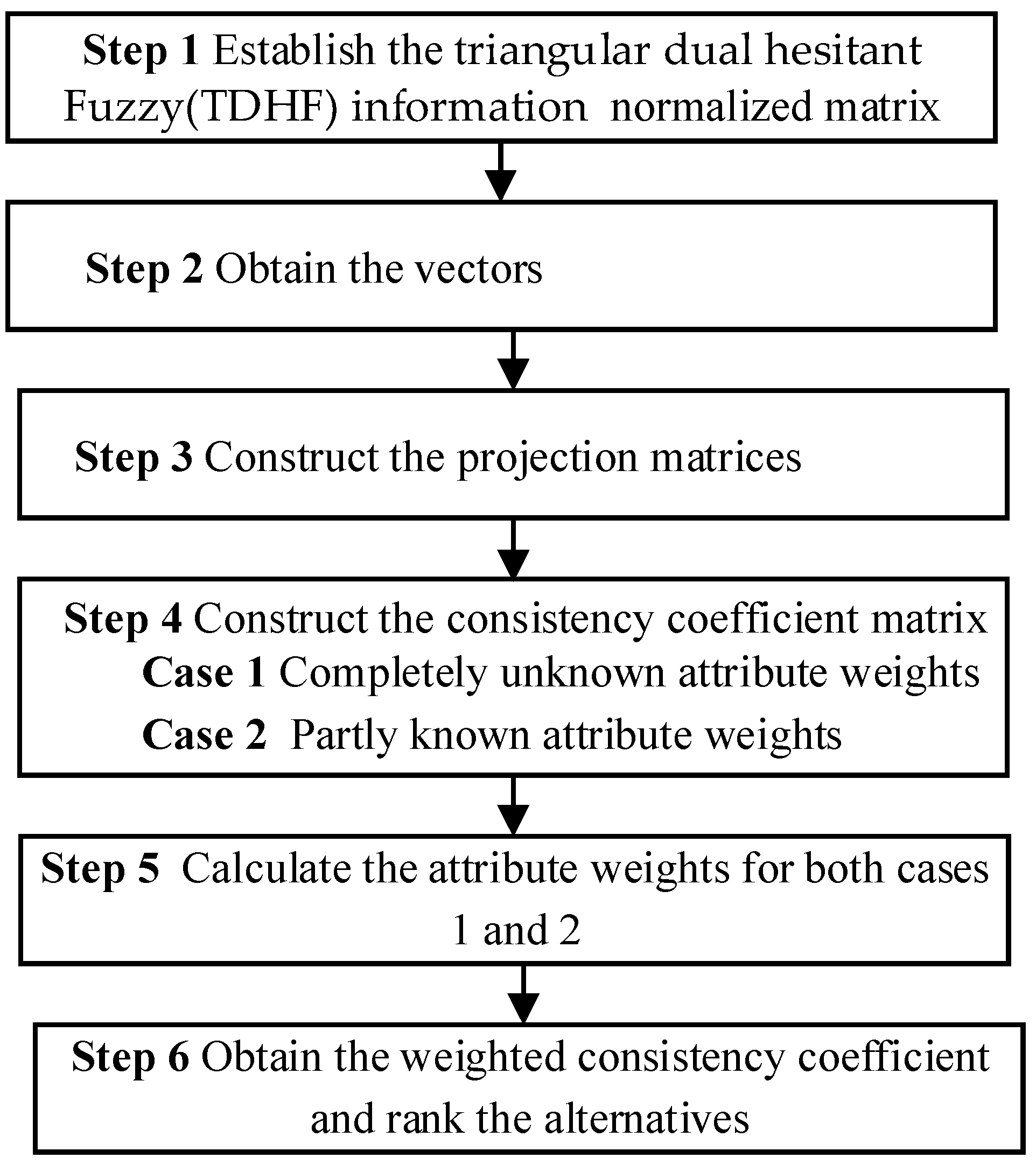
Based on this analysis, an approach is presented to address MADM issues where attribute weights (Aws) are either completely unknown or partially known, and the attribute values are expressed in the form of triangular dual hesitant fuzzy (TDHF) information. The presented sequence, titled ‘Bidirectional projection approach for triangular dual hesitant fuzzy multi-attribute decision-making,’ is outlined below, while Figure 1 shows a flowchart of the decision-making processes.

The algorithm is presented as follows:

Step 1. 

Establish the normalized matrix $\mathit{N}=({\overline{e}}_{ij}{)}_{m\times n}$ using Definition (8). If the decision matrix includes cost attributes, these must first be converted into benefit attributes according to Equation (20)

$$B=({\tilde{\overline{e}}}_{ij}{)}_{m\times n}=\left\{\begin{array}{c}{\cup }_{j\subset {\mathsf{\Omega }}_{{\rm B}}}\left\{\left\{[{\gamma }_{ij}^L,{\gamma }_{ij}^M,{\gamma }_{ij}^U]\right\},\left.\left\{[{\eta }_{ij}^L,{\eta }_{ij}^M,{\eta }_{ij}^U]\right\}\right\},\right.\\ {\cup }_{j\subset {\mathsf{\Omega }}_C}\left\{\left\{[{\eta }_{ij}^L,{\eta }_{ij}^M,{\eta }_{ij}^U]\right\},\left.\left\{[{\gamma }_{ij}^L,{\gamma }_{ij}^M,{\gamma }_{ij}^U]\right\}\right\},\right.\end{array}\right..$$

(20)

where Ω_B and Ω_C are the sets of benefit attributes and cost attributes, respectively, $i=1,2,\cdots ,m$ and $j=1,2,\cdots ,n$. Subsequently, construct the normalized matrix $\mathit{N}=({\overline{e}}_{ij}{)}_{m\times n}$ using Definition 10.

Step 2. 

Use Equation (10) to obtain the vectors $Y^{-}{Y}_i$, $Y^{-}{Y}^{+}$, and $Y_i{Y}^{+}$, where $i=1,2,\cdots ,m$.

Step 3. 

Use Equations (12) and (13) to construct the projection matrices $\mathrm{P}\mathrm{r}{\mathrm{j}}_{Y^{-}{Y}^{+}}(Y^{-}{Y}_i)$ and $\mathrm{P}\mathrm{r}{\mathrm{j}}_{Y_i{Y}^{+}}(Y^{-}{Y}^{+})$, where $i=1,2,\cdots ,m$.

Step 4. 

Use Equation (14) to construct the consistency coefficient matrix $\delta ={({\delta }_{ij})}_{m\times n}$, where $i=1,2,\cdots ,m$, $j=1,2,\cdots ,n$.

Step 5. 

Estimation of the attribute weights (Aws):

Case 1. 

If the attribute weights $w={(w_1,w_2,\cdots ,w_n)}^{\mathrm{T}}$ are completely unknown, they can be obtained from Equation (18);

Case 2. 

If the attribute weights $w={(w_1,w_2,\cdots ,w_n)}^{\mathrm{T}}$ are partially known, they can be calculated by solving Model (19).

Step 6. 

Aggregate the consistency coefficient and weights to obtain the weighted consistency coefficient ${\delta }_i(w)$. Rank the alternatives $Y_i$ according to the weighted consistency coefficient ${\delta }_i(w)$, where $i=1,2,\cdots ,m$.

5. An Illustrative Example

5.1. The Evaluation Steps Using the Consistent Bidirectional Projection Approach

This section presents two practical cases, Examples 2 and 3, to indicate the applicability of the algorithm presented in Section 4.

Example 2. 

Suppose an emerging company intends to choose the best supplier(s) from a set of alternatives $A_i(i=1,2,3,4)$. The performance of these suppliers is measured by the following three attributes: $G_1$—service capability; $G_2$—product quality; and $G_3$—innovation and development capability. The evaluation values are represented by TDHFEs. 

Table 1. TDHF decision matrix.

	${\mathit{G}}_1$	${\mathit{G}}_2$	${\mathit{G}}_3$
$Y_1$	$\left\{\left\{(0.2,0.3,0.4),(0.3,0.4,0.5),(0.5,0.6,0.7)\right\}\right.,$ $\left.\left\{(0.1,0.2,0.3),(0.2,0.3,0.4)\right\}\right\}$	$\left\{\left\{(0.3,0.4,0.5),(0.4,0.5,0.6)\right\}\right.,$ $\left.\left\{(0.1,0.2,0.3),(0.3,0.4,0.5)\right\}\right\}$	$\left\{\left\{(0.3,0.4,0.5),(0.4,0.5,0.6),(0.5,0.6,0.7)\right\}\right.,$ $\left.\left\{(0.1,0.2,0.3),(0.2,0.3,0.4)\right\}\right\}$
$Y_2$	$\left\{\left\{(0.3,0.4,0.5),(0.3,0.4,0.5),(0.5,0.6,0.7)\right\}\right.,$ $\left.\left\{(0.2,0.3,0.4)\right\}\right\}$	$\left\{\left\{(0.3,0.4,0.5),(0.2,0.3,0.4)\right\}\right.,$ $\left.\left\{(0.1,0.2,0.3),(0.4,0.5,0.6)\right\}\right\}$	$\left\{\left\{(0.1,0.2,0.3),(0.4,0.5,0.6),(0.5,0.6,0.7)\right\}\right.,$ $\left.\left\{(0.2,0.3,0.4),(0.3,0.4,0.5)\right\}\right\}$
$Y_3$	$\left\{\left\{(0.3,0.4,0.5),(0.4,0.5,0.6)\right\}\right.,$ $\left.\left\{(0.1,0.2,0.3),(0.3,0.4,0.5)\right\}\right\}$	$\left\{\left\{(0.2,0.3,0.4),(0.4,0.5,0.6),(0.5,0.6,0.7)\right\}\right.,$ $\left.\left\{(0.1,0.2,0.3),(0.2,0.3,0.4)\right\}\right\}$	$\left\{\left\{(0.3,0.4,0.5),(0.5,0.6,0.7),(0.6,0.7,0.8)\right\}\right.,$ $\left.\left\{(0.1,0.2,0.3),(0.2,0.3,0.4)\right\}\right\}$
$Y_4$	$\left\{\left\{(0.2,0.3,0.4),(0.4,0.5,0.6),(0.5,0.7,0.8)\right\}\right.,$ $\left.\left\{(0.1,0.2,0.3)\right\}\right\}$	$\left\{\left\{(0.4,0.5,0.6),(0.5,0.6,0.7)\right\}\right.,$ $\left.\left\{(0.1,0.2,0.3),(0.2,0.3,0.4)\right\}\right\}$	$\left\{\left\{(0.4,0.5,0.6),(0.6,0.7,0.8)\right\}\right.,$ $\left.\left\{(0.1,0.2,0.3),(0.2,0.3,0.4)\right\}\right\}$

 presents the decision matrix $\mathit{E}=({\tilde{e}}_{ij}{)}_{4\times 3}$.

Step 1. Construct the normalized matrix $\mathit{N}=({\tilde{e}}_{ij}{)}_{4\times 3}$, as presented in

Table 2. Normalized TDHF decision matrix.

	${\mathit{G}}_1$	${\mathit{G}}_2$	${\mathit{G}}_3$
$Y_1$	$\left\{\left\{(0.2,0.3,0.4),(0.3,0.4,0.5),(0.5,0.6,0.7)\right\}\right.,$ $\left.\left\{(0.1,0.2,0.3),(0.2,0.3,0.4)\right\}\right\}$	$\left\{\left\{(0.3,0.4,0.5),(0.3,0.4,0.5),(0.4,0.5,0.6)\right\}\right.,$ $\left.\left\{(0.1,0.2,0.3),(0.3,0.4,0.5)\right\}\right\}$	$\left\{\left\{(0.3,0.4,0.5),(0.4,0.5,0.6),(0.5,0.6,0.7)\right\}\right.,$ $\left.\left\{(0.1,0.2,0.3),(0.2,0.3,0.4)\right\}\right\}$
$Y_2$	$\left\{\left\{(0.3,0.4,0.5),(0.3,0.4,0.5),(0.5,0.6,0.7)\right\}\right.,$ $\left.\left\{(0.2,0.3,0.4),(0.2,0.3,0.4)\right\}\right\}$	$\left\{\left\{(0.2,0.3,0.4),(0.2,0.3,0.4),(0.3,0.4,0.5)\right\}\right.,$ $\left.\left\{(0.1,0.2,0.3),(0.4,0.5,0.6)\right\}\right\}$	$\left\{\left\{(0.1,0.2,0.3),(0.4,0.5,0.6),(0.5,0.6,0.7)\right\}\right.,$ $\left.\left\{(0.2,0.3,0.4),(0.3,0.4,0.5)\right\}\right\}$
$Y_3$	$\left\{\left\{(0.3,0.4,0.5),(0.3,0.4,0.5),(0.4,0.5,0.6)\right\}\right.,$ $\left.\left\{(0.1,0.2,0.3),(0.3,0.4,0.5)\right\}\right\}$	$\left\{\left\{(0.2,0.3,0.4),(0.4,0.5,0.6),(0.5,0.6,0.7)\right\}\right.,$ $\left.\left\{(0.1,0.2,0.3),(0.2,0.3,0.4)\right\}\right\}$	$\left\{\left\{(0.3,0.4,0.5),(0.5,0.6,0.7),(0.6,0.7,0.8)\right\}\right.,$ $\left.\left\{(0.1,0.2,0.3),(0.2,0.3,0.4)\right\}\right\}$
$Y_4$	$\left\{\left\{(0.2,0.3,0.4),(0.4,0.5,0.6),(0.5,0.7,0.8)\right\}\right.,$ $\left.\left\{(0.1,0.2,0.3),(0.1,0.2,0.3)\right\}\right\}$	$\left\{\left\{(0.4,0.5,0.6),(0.4,0.5,0.6),(0.5,0.6,0.7)\right\}\right.,$ $\left.\left\{(0.1,0.2,0.3),(0.2,0.3,0.4)\right\}\right\}$	$\left\{\left\{(0.4,0.5,0.6),(0.4,0.5,0.6),(0.6,0.7,0.8)\right\}\right.,$ $\left.\left\{(0.1,0.2,0.3),(0.2,0.3,0.4)\right\}\right\}$

. Additionally, assume that the decision-makers (DMs) are risk-averse.

Steps 2–3. Calculate the vectors $Y^{-}{Y}_i$, $Y^{-}{Y}^{+}$, and $Y_i{Y}^{+}$ using Equations (10) and (11). Then, use Equations (12) and (13) to form the projection matrices $\mathrm{P}\mathrm{r}{\mathrm{j}}_{Y^{-}{Y}^{+}}(Y^{-}{Y}_i)$ and $\mathrm{P}\mathrm{r}{\mathrm{j}}_{Y_i{Y}^{+}}(Y^{-}{Y}^{+})$, where $i=1,2,3,4$. The matrices $\mathrm{P}\mathrm{r}{\mathrm{j}}_{Y^{-}{Y}^{+}}(Y^{-}{Y}_i)$ and $\mathrm{P}\mathrm{r}{\mathrm{j}}_{Y_i{Y}^{+}}(Y^{-}{Y}^{+})$ are described as follows:

$$\begin{gathered} \mathrm{P}\mathrm{r}{\mathrm{j}}_{Y^{-}{Y}^{+}}(Y^{-}{Y}_i)=\left(\begin{array}{ccc}0.0170& 0.0173& 0.0267\\ 0.0170& 0.0116& 0\\ 0.0073& 0.0231& 0.2890\\ 0.0280& 0.0231& 0.0400\end{array}\right), \\ \mathrm{P}\mathrm{r}{\mathrm{j}}_{Y_i{Y}^{+}}(Y^{-}{Y}^{+})=\left(\begin{array}{ccc}0.0371& 0.0334& 0.0222\\ 0.0371& 0.0667& 0\\ 0& 0.0222& 0.0250\\ 0.0191& 0.0111& 0\end{array}\right) \end{gathered}$$

Step 4. Use Equation (14) to construct the consistency coefficient matrix $\delta ={({\delta }_{ij})}_{4\times 3}$ as follows:

$$\delta ={({\delta }_{ij})}_{4\times 3}=\left(\begin{array}{ccc}0.4897& 0.4918& 0.5023\\ 0.4897& 0.4713& 0.5000\\ 0.5037& 0.5004& 0.5020\\ 0.5046& 0.5061& 0.5204\end{array}\right).$$

Case 1. For completely unknown attribute weights (Aws), proceed with the following steps:

Step 5. From Equation (18), the Aws are determined as $w={(0.3323,0.3294,0.3385)}^{\mathrm{T}}$;

Step 6. Aggregate the consistency coefficients and weights to obtain the weighted consistency coefficients, where ${\delta }_i(w)$ and $i=1,2,3,4$:

$${\delta }_1(w)=1.4838, {\delta }_2(w)=1.4611, {\delta }_3(w)=1.5061, \mathrm{and} {\delta }_4(w)=1.5311.$$

(21)

Rank the alternatives according to the weighted consistency coefficient, where $i=1,2,3,4$, obviously $Y_4\succ Y_3\succ Y_1$ $\succ Y_2$; then, the best desirable alternative is Y₄.

Case 2. For partly known attribute weights, assume the following:

$$\Delta =\left\{0.15\le w_1\le 0.2,0.3\le w_2\le 0.35,\right.\left.0.4\le w_3\le 0.55\right\}.$$

Step 5′. Use Model (19) to establish the single-objective model defined by the following:

$$\begin{array}{l}\max ({\delta }_i)=1.9887w_1+1.9697w_2+2.0247w_3\\ \mathrm{s}.\mathrm{t} \Delta , {\displaystyle \sum _{j=1}^n{w}_j=1,}{w}_j\ge 0, j=1,2,\cdots ,n.\end{array}$$

By solving Model (19), the Aws are determined as $w={(0.15,0.30,0.55)}^{\mathrm{T}}$.

Step 6’. Aggregate the consistency coefficients and weights to obtain the following weighted consistency coefficients ${\delta }_i(w)$, where $i=1,2,3,4$:

$${\delta }_1(w)=1.6026, {\delta }_2(w)=1.5800, {\delta }_3(w)=1.6250, \mathrm{and} {\delta }_4(w)=1.6487.$$

Rank the alternatives according to the weighted consistency coefficient, and obviously, $Y_4\succ Y_3\succ Y_1\succ Y_2$; then, the best desirable alternative is Y₄.

5.2. Comparison

To evaluate the presented approach’s efficiency and feasibility, we use an example adopted from [24] to show how the proposed approach can overcome the disadvantages of Zhang’s [46], Ju et al.’s [24], and Zang et al.’s [25] methods.

Example 3. 

Consider a classical multi-attribute decision-making (MADM) problem that deals with the selection of an investment company. There is a set of alternatives: (1) A₁ is a car company; (2) A₂ is a food company; (3) A₃ is a computer company; (4) A₄ is an arms company. The investment company must make a decision by the following three attributes: (1) G₁ is the risk analysis; (2) G₂ is the growth analysis; (3) G₃ is the environmental impact analysis. The comprehensive and weight values are completely unknown, with w = (0.3323, 0.3294, 0.3386)^T. It should be specially explained that G₁ and G₃ are the cost attributes, and G₂ is the benefit attribute. Triangular dual hesitant fuzzy elements (TDHFEs) are used to measure the evaluation values.

Table 3. TDHF decision matrix.

	${\mathit{G}}_1$	${\mathit{G}}_2$	${\mathit{G}}_3$
$Y_1$	$\left\{\left\{(0.1,0.2,0.3),(0.2,0.3,0.4)\right\}\right.,$ $\left.\left\{(0.3,0.4,0.5),(0.4,0.5,0.6),(0.5,0.6,0.7)\right\}\right\}$	$\left\{\left\{(0.3,0.4,0.5),(0.4,0.5,0.6)\right\}\right.,$ $\left.\left\{(0.2,0.3,0.4),(0.4,0.5,0.6)\right\}\right\}$	$\left\{\left\{(0.1,0.2,0.3),(0.2,0.3,0.4)\right\}\right.,$ $\left.\left\{(0.3,0.4,0.5),(0.4,0.5,0.6),(0.5,0.6,0.7)\right\}\right\}$
$Y_2$	$\left\{\left\{(0.3,0.4,0.5)\right\}\right.,$ $\left.\left\{(0.4,0.5,0.6),(0.5,0.6,0.7)\right\}\right\}$	$\left\{\left\{(0.3,0.4,0.5),(0.4,0.5,0.6)\right\}\right.,$ $\left.\left\{(0.2,0.3,0.4),(0.4,0.5,0.6)\right\}\right\}$	$\left\{\left\{(0.2,0.3,0.4),(0.3,0.4,0.5)\right\}\right.,$ $\left.\left\{(0.2,0.3,0.4),(0.4,0.5,0.6),(0.5,0.6,0.7)\right\}\right\}$
$Y_3$	$\left\{\left\{(0.2,0.3,0.4),(0.3,0.4,0.5)\right\}\right.,$ $\left.\left\{(0.3,0.4,0.5),(0.4,0.5,0.6)\right\}\right\}$	$\left\{\left\{(0.2,0.3,0.4),(0.4,0.5,0.6),(0.5,0.6,0.7)\right\}\right.,$ $\left.\left\{(0.1,0.2,0.3),(0.2,0.3,0.4)\right\}\right\}$	$\left\{\left\{(0.1,0.2,0.3),(0.2,0.3,0.4)\right\}\right.,$ $\left.\left\{(0.4,0.5,0.6),(0.5,0.6,0.7),(0.6,0.7,0.8)\right\}\right\}$
$Y_4$	$\left\{\left\{(0.1,0.2,0.3)\right\}\right.,$ $\left.\left\{(0.3,0.4,0.5),(0.4,0.5,0.6),(0.6,0.7,0.8)\right\}\right\}$	$\left\{\left\{(0.4,0.5,0.6),(0.5,0.6,0.7)\right\}\right.,$ $\left.\left\{(0.2,0.3,0.4),(0.3,0.4,0.5)\right\}\right\}$	$\left\{\left\{(0.1,0.2,0.3),(0.2,0.3,0.4)\right\}\right.,$ $\left.\left\{(0.4,0.5,0.6),(0.6,0.7,0.8)\right\}\right\}$

presents the decision matrix $\mathit{E}=({\tilde{e}}_{ij}{)}_{4\times 3}$.

First, establish the normalized matrix $\mathit{N}=({\overline{e}}_{ij}{)}_{4\times 3}$ using Definition 10, as presented in

Table 4. Normalized TDHF decision matrix.

	${\mathit{G}}_1$	${\mathit{G}}_2$	${\mathit{G}}_3$
$Y_1$	$\left.\left\{(0.3,0.4,0.5),(0.4,0.5,0.6),(0.5,0.6,0.7)\right\}\right\},$$\left\{\left\{(0.1,0.2,0.3),(0.2,0.3,0.4)\right\}\right.$	$\left\{\left\{(0.3,0.4,0.5),(0.3,0.4,0.5),(0.4,0.5,0.6)\right\}\right.,$ $\left.\left\{(0.2,0.3,0.4),(0.4,0.5,0.6)\right\}\right\}$	$\left.\left\{(0.3,0.4,0.5),(0.4,0.5,0.6),(0.5,0.6,0.7)\right\}\right\}$$\left\{\left\{(0.1,0.2,0.3),(0.2,0.3,0.4)\right\}\right.,$
$Y_2$	$\left.\left\{(0.4,0.5,0.6),(0.4,0.5,0.6),(0.5,0.6,0.7)\right\}\right\},$$\left\{\left\{(0.3,0.4,0.5),(0.3,0.4,0.5)\right\}\right.$	$\left\{\left\{(0.3,0.4,0.5),(0.3,0.4,0.5),(0.4,0.5,0.6)\right\}\right.,$ $\left.\left\{(0.2,0.3,0.4),(0.4,0.5,0.6)\right\}\right\}$	$\left.\left\{(0.2,0.3,0.4),(0.4,0.5,0.6),(0.5,0.6,0.7)\right\}\right\}$$\left\{\left\{(0.2,0.3,0.4),(0.3,0.4,0.5)\right\}\right.,$
$Y_3$	$\left.\left\{(0.3,0.4,0.5),(0.3,0.4,0.5),(0.4,0.5,0.6)\right\}\right\},$$\left\{\left\{(0.2,0.3,0.4),(0.3,0.4,0.5)\right\}\right.$	$\left\{\left\{(0.2,0.3,0.4),(0.4,0.5,0.6),(0.5,0.6,0.7)\right\}\right.,$ $\left.\left\{(0.1,0.2,0.3),(0.2,0.3,0.4)\right\}\right\}$	$\left.\left\{(0.4,0.5,0.6),(0.5,0.6,0.7),(0.6,0.7,0.8)\right\}\right\}$$\left\{\left\{(0.1,0.2,0.3),(0.2,0.3,0.4)\right\}\right.,$
$Y_4$	$\left.\left\{(0.3,0.4,0.5),(0.4,0.5,0.6),(0.6,0.7,0.8)\right\}\right\}$$\left\{\left\{(0.1,0.2,0.3)\right\}\right.,$	$\left\{\left\{(0.4,0.5,0.6),(0.4,0.5,0.6),(0.5,0.6,0.7)\right\}\right.,$ $\left.\left\{(0.2,0.3,0.4),(0.3,0.4,0.5)\right\}\right\}$	$\left.\left\{(0.4,0.5,0.6),(0.4,0.5,0.6),(0.6,0.7,0.8)\right\}\right\}$$\left\{\left\{(0.1,0.2,0.3),(0.2,0.3,0.4)\right\}\right.,$

. Additionally, assume that the decision-makers (DMs) are risk-averse, G₁ and G₃ are the cost attributes, and attribute type conversion is required.

Then,

Table 5. Comprehensive values and ranking orders by various approaches.

Approach	$\mathbf{Comprehensive} \mathbf{Values} \mathbf{of} \mathit{\delta }({\mathit{y}}_{\mathit{i}})$$(\mathit{i}=1,2,3,4)$	Rankings
Zhang’s [46] approach using a distance and entropy measure	$\delta (y_1)=0.0915$, $\delta (y_2)=0.0423$, $\delta (y_3)=0.1140$, $\delta (y_4)=0.1569$	$Y_4\succ Y_3\succ Y_1\succ Y_2$
Ju et al.’s [24] approach using a simple weighted averaging operator	$\delta (y_1)=0.2745$, $\delta (y_2)=0.2537$, $\delta (y_3)=0.2397$, $\delta (y_4)=0.2307$	$Y_1\succ Y_2\succ Y_3\succ Y_4$
Zang et al.’s [25] approach using the IVDHFWHM operator	$\delta (y_1)=0.4567$, $\delta (y_2)=0.2563$, $\delta (y_3)=0.3526$, $\delta (y_4)=0.3016$	$Y_1\succ Y_3\succ Y_4\succ Y_2$
The proposed method for completely unknown attribute weights	$\delta (y_1)=1.4838$, $\delta (y_2)=1.4611$, $\delta (y_3)=1.5061$, $\delta (y_4)=1.5311$	$Y_4\succ Y_3\succ Y_1\succ Y_2$

shows the comprehensive values $\delta (y_i)$ of the alternatives A_i (i = 1, 2, 3, 4) as calculated by the different methods [24,25,46].

From Table 5, it can be observed that our proposed method yields the same ranking results as the method by Zhang [46], although the value differences among the four alternatives are inconsistent. Additionally, there are discrepancies in the ranking results when comparing our method with those proposed by Ju et al. [24] and Zang et al. [25]. To clarify these differences, we will conduct a detailed analysis.

• Comparison with Zhang’s method [46]: Zhang’s method [46] is based on distance and entropy measures, while our approach integrates consistent bidirectional projection measures with the TOPSIS method. The similarity in ranking results and differences in values can be attributed to two main factors: (1) Our consistent bidirectional projection measure considers not only the distance and angle between evaluated objects but also the bidirectional projection magnitudes. Zhang’s method [46], being based on distance and entropy, shares some commonalities with our approach in terms of evaluating closeness to positive and negative ideal points. (2) Both methods select positive ideal points (PIPs) and negative ideal points (NIPs) among the alternatives. In Zhang’s method [46], the PIP and NIP are set as {{1}, {0}} and {{0}, {1}}, respectively. These similarities in approach result in the same ranking outcomes and value differences, thus demonstrating the effectiveness and feasibility of our method;
• Comparison with the methods from Ju et al. [24] and Zang et al. [25]: Significant differences in ranking results and attribute values are observed between our method and the approaches by Ju et al. [24] and Zang et al. [25]. The discrepancy arises because the simple weighted averaging operator in Ju et al. [24] and the IVDHFWHM operator in Zang et al. [25] primarily focus on the closeness to positive ideal points (PIPs), neglecting the distance from negative ideal points (NIPs). In contrast, our consistent bidirectional projection algorithm ensures that the optimal alternative is not only close to the PIPs but also sufficiently distant from the NIPs. Consequently, these differences in methodology lead to varying ranking results. This analysis supports the conclusion that our proposed method is more effective and feasible for practical decision-making problems.

The main advantages of the proposed method are outlined as follows:

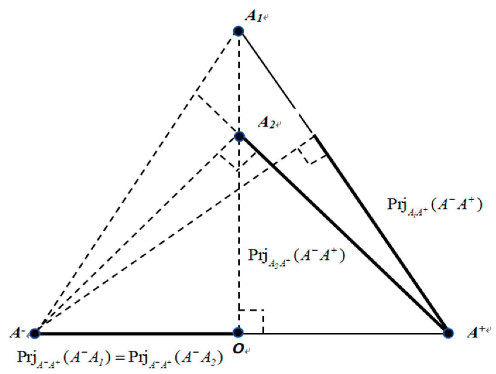
• The proposed method exhibits higher discrimination and sensitivity, particularly when dealing with alternatives that have small numerical differences. The consistent bidirectional projection method outperforms existing approaches by being more sensitive to such nuances. This is primarily because it measures the relative closeness of alternatives to positive and negative ideal points rather than relying solely on absolute numerical differences, thereby minimizing information loss. In cases where the distances between alternatives and both the positive and negative ideal points are equal, the TOPSIS method may yield identical results, making it difficult to identify the best alternative. However, the bidirectional projection method can effectively resolve this issue, providing a clear distinction among alternatives. As presented in Figure 2, when d(A₁A⁺) = d(A₂A⁺), d(A₁A⁻) = d(A₂A⁻), the method in this paper has a good degree of differentiation, and our method demonstrates superior differentiation;
• Comprehensive consideration of triangular dual hesitant fuzzy (TDHF) information: The consistent bidirectional projection method offers a more comprehensive approach to handling triangular dual hesitant fuzzy information. It not only accounts for the projection distance and the included angle between evaluated objects but also considers the bidirectional projection magnitudes, membership degree, and non-membership degree;
• Comprehensive consideration of the consistency change with PIPs and NIPs: The consistent bidirectional projection method takes into account both the relationship between alternatives and the positive and negative ideal points as well as the relationship between consistency changes and the included angle. This makes the proposed multiple-attribute decision-making method—which is based on triangular dual hesitant fuzzy elements—both reasonable and effective.

6. Conclusions

Dual hesitant fuzzy sets (DHFSs) and interval-valued dual hesitant fuzzy sets (IVDHFSs) are powerful tools for capturing decision-makers’ (DMs’) hesitancy and uncertainty in the multi-attribute decision-making (MADM) process, incorporating hesitant functions with membership degrees (MDs) and non-membership degrees (NMDs). However, the requirement that the membership function be expressed as crisp or interval numbers limits their application and flexibility. Inspired by triangular numbers and hesitant triangular fuzzy sets (HTFSs), this work introduces a novel approach by relaxing the form of the membership function and presenting triangular dual hesitant fuzzy sets (TDHFSs) to better handle the fuzziness and uncertainty inherent in triangular information. The proposed TDHFSs retain the strengths and versatility of THFSs and DHFSs.

First, the new concept of TDHFEs is presented. The operational laws of TDHFEs are utilized to develop some projection and bidirectional projection measures for combining the triangular hesitant fuzzy data. Additionally, the consistent bidirectional projection decision-making approach is investigated to solve the consistency issue as a projection on the positive ideal points (PIPs) and negative ideal points (NIPs). Furthermore, the optimization models are established using the maximizing consistency coefficient approach to determine completely or partially unknown attribute weights. According to the presented consistently bidirectional projection decision-making approach and attribute weight estimation method, an approach is presented under a triangular dual hesitant fuzzy environment. Finally, a practical example is presented for the supplier choosing supply chain management to describe the presented approach’s applicability and effectiveness, and comparative analyses are implemented to reveal the presented approach’s feasibility and efficiency.

Based on the above analysis, the primary advantages of this proposed consistent bidirectional projection can be summarized as follows: (1) The consistency and correlation coefficients for triangular dual hesitant fuzzy sets (TDHFSs) have been developed. We explain and prove the desirable properties of the proposed coefficient, such as boundary conditions and symmetry; (2) we define the vector and projection vector for alternatives with triangular dual hesitant fuzzy information. Furthermore, we introduce a consistent bidirectional projection decision-making method that considers not only the projection of alternatives on positive ideal points (PIPs) and negative ideal points (NIPs) but also the distance, angle, and degree of incidence consistency between the alternatives and ideal points; (3) the completely unknown weights of attributes are determined by a consistency coefficient maximization optimization model. Additionally, partially known attribute weights can be derived from a constrained optimization model based on the available weight information.

For future research, the following areas are worthy of further exploration: (1) The bidirectional projection method for TDHFSs warrants deeper investigation. In more complex decision-making environments, we could consider incorporating DMs’ attitudes and attribute preferences into the bidirectional projection method; (2) the proposed bidirectional projection method could be integrated with various operators to capture more decision information, such as the power average (PA) operator, Heronian operator, Einstein operations, and so on. Additionally, it could be combined with other traditional MADM methods, including the TODIM, ELECTRE, PROMETHEE, and QUALIFLEX methods; (3) the proposed bidirectional projection method also has potential applications in emerging fields, such as intelligent decision-making.

References

1. Zadeh, L.A. Fuzzy Sets. Inf. Control 1965, 8, 338–353. [Google Scholar] [CrossRef]
2. Karnik, N.N.; Mendel, J.M. Operations on Type-2 Fuzzy Sets. Fuzzy Sets Syst. 2001, 122, 327–348. [Google Scholar] [CrossRef]
3. Atanassov, K.T. More on Intuitionistic Fuzzy Sets. Fuzzy Sets Syst. 1989, 33, 37–45. [Google Scholar] [CrossRef]
4. Atanassov, K.T.; Gargov, G. Interval Valued Intuitionistic Fuzzy Sets. Fuzzy Sets Syst. 1989, 31, 343–359. [Google Scholar] [CrossRef]
5. Gau, W.L.; Buehrer, D.J. Vague Sets. IEEE Trans. Syst. Man Cybern. 1993, 23, 610–614. [Google Scholar] [CrossRef]
6. Bustince, H.; Burillo, P. Vague Sets Are Intuitionistic Fuzzy Sets. Fuzzy Sets Syst. 1996, 79, 403–405. [Google Scholar] [CrossRef]
7. Smarandache, F. N-Valued Refined Neutrosophic Logic and Its Applications to Physics. Prog. Phys. 2014, 9, 143–146. [Google Scholar]
8. Peng, X.; Yang, Y. Some Results for Pythagorean Fuzzy Sets. Int. J. Intell. Syst. 2015, 11, 1133–1160. [Google Scholar] [CrossRef]
9. Wei, G.W. Pythagorean Fuzzy Hamacher Power Aggregation Operators in Multiple Attribute Decision Making. Fundam. Inform. 2019, 1, 57–85. [Google Scholar] [CrossRef]
10. Torra, V. Hesitant Fuzzy Sets. Int. J. Intell. Syst. 2010, 25, 529–539. [Google Scholar] [CrossRef]
11. Rodríguez, R.M.; Martínez, L.; Torra, V.; Xu, Z.S.; Herrera, F. Hesitant Fuzzy Sets: State of the Art and Future Directions. Int. J. Intell. Syst. 2014, 6, 495–524. [Google Scholar] [CrossRef]
12. Farhadinia, B. A Series of Score Functions for Hesitant Fuzzy Sets. Inf. Sci. 2014, 277, 102–110. [Google Scholar] [CrossRef]
13. Farhadinia, B. Information Measures for Hesitant Fuzzy Sets and Interval-Valued Hesitant Fuzzy Sets. Inf. Sci. 2013, 240, 129–144. [Google Scholar] [CrossRef]
14. Xia, M.; Xu, Z. Hesitant Fuzzy Information Aggregation in Decision Making. Int. J. Approx. Reason. 2011, 52, 395–407. [Google Scholar] [CrossRef]
15. Xu, Z.; Xia, M. On Distance and Correlation Measures of Hesitant Fuzzy Information. Int. J. Intell. Syst. 2011, 26, 410–425. [Google Scholar] [CrossRef]
16. Peng, D.H.; Gao, C.Y.; Gao, Z.F. Generalized Hesitant Fuzzy Synergetic Weighted Distance Measures and Their Application to Multiple Criteria Decision-Making. Appl. Math. Model. 2013, 37, 5837–5850. [Google Scholar] [CrossRef]
17. Xu, Z.; Xia, M. Hesitant Fuzzy Entropy and Cross-Entropy and Their Use in Multiattribute Decision-Making. Int. J. Intell. Syst. 2012, 27, 799–822. [Google Scholar] [CrossRef]
18. Xu, Z.; Zhang, X. Hesitant Fuzzy Multi-Attribute Decision Making Based on TOPSIS with Incomplete Weight Information. Knowl.-Based Syst. 2013, 52, 53–64. [Google Scholar] [CrossRef]
19. Zhang, X.; Xu, Z. The TODIM Analysis Approach Based on Novel Measured Functions under Hesitant Fuzzy Environment. Knowl.-Based Syst. 2014, 61, 48–58. [Google Scholar] [CrossRef]
20. He, Y.; He, Z.; Wang, G. Hesitant Fuzzy Power Bonferroni Means and Their Application to Multiple Attribute Decision Making. IEEE Trans. Fuzzy Syst. 2015, 23, 1655–1668. [Google Scholar] [CrossRef]
21. Chen, N.; Xu, Z.; Xia, M. Interval-Valued Hesitant Preference Relations and Their Applications to Group Decision Making. Knowl.-Based Syst. 2013, 37, 528–540. [Google Scholar] [CrossRef]
22. Wei, G.; Zhao, X.; Lin, R. Induced Hesitant Interval-Valued Fuzzy Einstein Aggregation Operators and Their Application to Multiple Attribute Decision Making. J. Intell. Fuzzy Syst. 2013, 46, 43–53. [Google Scholar] [CrossRef]
23. Zhu, B.; Xu, Z.; Xia, M. Dual Hesitant Fuzzy Sets. J. Appl. Math. 2012, 2012, 879629. [Google Scholar] [CrossRef]
24. Ju, Y.; Liu, X.; Yang, S. Interval-Valued Dual Hesitant Fuzzy Aggregation Operators and Their Applications to Multiple Attribute Decision Making. J. Intell. Fuzzy Syst. 2014, 27, 1203–1218. [Google Scholar] [CrossRef]
25. Zang, Y.; Zhao, X.; Li, S. Interval-Valued Dual Hesitant Fuzzy Heronian Mean Aggregation Operators and Their Application to Multi-Attribute Decision Making. Int. J. Comput. Intell. Appl. 2018, 2018, 1850005. [Google Scholar] [CrossRef]
26. Su, Z.; Xu, Z. Distance and Similarity Measures for Dual Hesitant Fuzzy Sets and Their Applications in Pattern Recognition. J. Intell. Fuzzy Syst. 2015, 29, 731–745. [Google Scholar] [CrossRef]
27. Liao, H.; Xu, Z. A VIKOR-Based Method for Hesitant Fuzzy Multi-Criteria Decision Making. Fuzzy Optim. Decis. Mak. 2013, 12, 373–392. [Google Scholar] [CrossRef]
28. Zhang, N.; Wei, G. Extension of VIKOR Method for Decision Making Problem Based on Hesitant Fuzzy Set. Appl. Math. Model. 2013, 37, 4938–4947. [Google Scholar] [CrossRef]
29. Zhang, X.; Xu, Z. Hesitant Fuzzy QUALIFLEX Approach with a Signed Distance-Based Comparison Method for Multiple Criteria Decision Analysis. Expert Syst. Appl. 2015, 42, 873–884. [Google Scholar] [CrossRef]
30. Xu, Z.; Da, Q. Projection Method for Uncertain Multi-Attribute Decision Making with Preference Information on Alternatives. Int. J. Inf. Technol. Decis. Mak. 2004, 3, 429–434. [Google Scholar] [CrossRef]
31. Zhou, H.A.; Liu, S.Y. Projection Method of Fuzzy Multi-Attribute Decision-Making Based on the Maximal Deviation Model. Syst. Eng. Electron. 2007, 27, 741–744. [Google Scholar]
32. Hua, X.Y.; Tan, J.X. Revised TOPSIS Method Based on Vertical Projection Distance-Vertical Projection Method. Syst. Eng. Theory Pract. 2004, 24, 114–119. [Google Scholar]
33. Liu, X.D.; Zhu, J.J.; Liu, S.F. Bidirectional Projection Method with Hesitant Fuzzy Information. Syst. Eng. Theory Pract. 2014, 34, 2637–2644. [Google Scholar]
34. Ye, J. Bidirectional Projection Method for Multiple Attribute Group Decision Making with Neutrosophic Numbers. Neural Comput. Appl. 2015, 28, 1021–1029. [Google Scholar] [CrossRef]
35. Liu, P.; Li, Y.; Teng, F. Bidirectional Projection Method for Probabilistic Linguistic Multi-Criteria Group Decision-Making Based on Power Average Operator. Int. J. Fuzzy Syst. 2019, 21, 2340–2353. [Google Scholar] [CrossRef]
36. Liu, P.; You, X. Bidirectional Projection Measure of Linguistic Neutrosophic Numbers and Their Application to Multi-Criteria Group Decision Making. Comput. Ind. Eng. 2019, 128, 447–457. [Google Scholar] [CrossRef]
37. Yu, Y.; Liu, Z. Multi-Dimensionality Reputation Evaluation Model for C2C E-Commerce in Hesitant Triangular Fuzzy Setting. J. Intell. Fuzzy Syst. 2019, 37, 1809–1817. [Google Scholar] [CrossRef]
38. Zhao, X.; Lin, R.; Wei, G. Hesitant Triangular Fuzzy Information Aggregation Based on Einstein Operations and Their Application to Multiple Attribute Decision Making. Expert Syst. Appl. 2014, 41, 1086–1094. [Google Scholar] [CrossRef]
39. Van Laarhoven, P.J.M.; Pedrycz, W. A Fuzzy Extension of Saaty’s Priority Theory. Fuzzy Sets Syst. 1983, 11, 229–241. [Google Scholar] [CrossRef]
40. Xu, Z.S.; Da, Q.L. The Uncertain OWA Operator. Int. J. Intell. Syst. 2002, 17, 569–575. [Google Scholar] [CrossRef]
41. Gerstenkorn, T.; Mańko, J. Correlation of Intuitionistic Fuzzy Sets. Fuzzy Sets Syst. 1991, 44, 39–43. [Google Scholar] [CrossRef]
42. Bustince, H.; Burillo, P. Correlation of Interval-Valued Intuitionistic Fuzzy Sets. Fuzzy Sets Syst. 1995, 74, 237–244. [Google Scholar] [CrossRef]
43. Meng, F.; Chen, X. Correlation Coefficients of Hesitant Fuzzy Sets and Their Application Based on Fuzzy Measures. Cogn. Comput. 2015, 7, 445–463. [Google Scholar] [CrossRef]
44. Wu, W.; Chen, H.; Zhou, L. Correlation Coefficient of Interval-Valued Dual Hesitant Fuzzy Set and Its Application. Comput. Eng. Appl. 2014, 51, 140–144. [Google Scholar]
45. Ando, T. Geometric Mean and Norm Schwarz Inequality. Ann. Funct. Anal. 2016, 7, 1–8. [Google Scholar] [CrossRef]
46. Zhang, H. Distance and Entropy Measures for Dual Hesitant Fuzzy Sets. Comput. Appl. Math. 2020, 39, 91. [Google Scholar] [CrossRef]
Figure 1. A flowchart of the proposed bidirectional projection approach for TDHF multi-attribute decision-making.
Axioms 13 00618 g001
Figure 2. Schematic diagram of consistent bidirectional projection.
Axioms 13 00618 g002