Analytical and Numerical Approaches via Quadratic Integral Equations

Abstract

A quadratic integral Equation (QIE) of the second kind with continuous kernels is solved in the space $C\left(\right[0,T]\times [0,T\left]\right).$ The existence of at least one solution to the QIE is discussed in this article. Our evidence depends on a suitable combination of the measures of the noncompactness approach and the fixed-point principle of Darbo. The quadratic integral equation can be used to derive a system of integral equations of the second kind using the quadrature method. With the aid of two different polynomials, Laguerre and Hermite, the system of integral equations is solved using the collocation method. In each numerical approach, the estimation of the error is discussed. Finally, using some examples, the accuracy and scalability of the proposed method are demonstrated along with comparisons. Mathematica 11 was used to obtain all of the results from the techniques that were shown.

1. Introduction

Integral equations of various types play an important role in many branches of linear and nonlinear functional analysis and their applications, which appear in many different applied science fields. For example, in [1], Alhazmi solved the mixed integral equation of the first kind using a novel approach, Ghiat et al. [2] solved the non-linear Volterra integral equation of the first kind using a block-by-block technique, in [3], Gong et al. focused on an optimal control problem in a confined domain that includes a wave equation constraint across the whole space, Jaabar and Hussain solved Volterra integral equations using the definition of a new transformation (the Al-Zughair Transform) in [4], the unique solution and existence of the nonlinear Volterra–Fredholm integral equation of the second kind were examined by Matoog et al. in [5], Ma and Huang created a collocation technique for VIE of the third kind solutions in [6], a form of Volterra functional integral Equations (VIEs) of the second kind in which both limits of integration are variables was examined by Micula in [7] using an iterative numerical approach, Micula presented a simple numerical technique for estimating solutions to Fredholm-–Volterra integral equations of the second kind in [8], and Sarkar et al. presented a method for resolving a nonlinear Fredholm integral equation with a constant delay in [9]. Quadratic integral equations are complex equations in the science of integral equations due to the difficulty of obtaining an exact solution, but they have many applications in life sciences, so researchers have been interested in finding an approximate solution to this type of equation. For example, we can cite the meshless method in Fatahi [10], the homotopy perturbation method in Noeiaghdam et al. [11], the collocation method in Jaan [12], the Chebyshev polynomial method in Abusalim et al. [13], the Legendre polynomials method in Abdel-Aty and Abdou [14], the block–pulse and hybrid functions in Abusalim et al. [15], the wavelet method in Adibi et al. [16], and the resolvent kernel method in Abdel-Aty et al. [17]. To find an approximate solution to this type of equation, researchersfound new algorithms, that use a linear combination of functions with an orthogonal or non-orthogonal basis and polynomials as an expression of the solution, for example, Fibonacci polynomials in Mirzaee and Hoseini [18], block–pulse functions in Hesameddini and Shahbazi [19], Chebyshev polynomials in Alhazmi [20], hat functions in Mirzaee and Hadadiyan [21], Bernoulli polynomials in Bazm [22], and the operational matrix method in Mirzaee and Samadyar [23].

Quadratic integral equations are a special type of integral equations that appear in many mathematical models of various phenomena in the real world. Numerous mathematical physics and chemical engineering problems at times involve quadratic integral equations, such as the theory of kinetic gases, the theory of radiative transfer, the traffic theory, the queuing theory, the theory of neutron transport, and many other applications [24,25,26]. See Abdou et al. [27], El-Sayed et al. [28], Abdel-Aty [29], and Mirzaee [30] for studies on the existence of a solution and a numerical approach to solve this kind of integral equations. Volterra-type singular quadratic integral equations have recently attracted a lot of attention due to their importance in describing problems that appear in basic sciences and various events in the real world.

In many branches of nonlinear analysis, special measures of specific incompatibilities are often used. Arab et al. [31] found this technique a really useful tool within the existence theorems of many kinds of integral equations. The purpose of this study is to prove the existence theorem for a nonlinear integral equation using the method of special measures of noncompactness and a fixed-point theory of the Darbo type in the class $C[0,T]$. The results conferred during this article appear to be new and original. The result obtained within the article generalizes a lot of results obtained earlier in many papers, such as Abdel-Aty et al. [17] and Basseem [32].

In this paper, we will discuss the solvability of the following quadratic integral equation:

$$\begin{array}{cc}\hfill \mu \mathrm{\Phi }(x,t)=g(x,t)& +E_1\left(x,t,{\int }_0^{t}f(x,\tau )\mathrm{\Phi }(x,\tau )\mathrm{d}\tau \right)\hfill \\ \hfill & \times E_2\left(x,t,{\int }_0^{x}k(y,t)\mathrm{\Phi }(y,t)\mathrm{d}y\right),\mathrm{for}(x,t)\in ([0,T]\times [0,T]),\hfill \end{array}$$

(1)

where $\mu$ is a constant, $\mathrm{\Phi }(x,t)$ is unknown function in Banach space $C\left(\right[0,T]\times [0,T\left]\right);T<1$. The kernels $f(x,\tau )$, $k(y,t)$ are continuous in $C\left(\right[0,T]\times [0,T\left]\right)$; in addition, the given $g(x,t)$ is a continuous function in the same class.

The rest of this paper is organized as follows: In Section 2, the initial principles are reviewed by mentioning some important definitions and theorems in the noncompactness measure. In Section 3, in light of the fixed-point theorem and the contradiction measure and under certain conditions, we obtain the basic condition for the existence of at least one solution to the quadratic integral equation Equation (1). This solution is positive and belongs to the used branch. This is formulated by stating a basic theorem for the existence of at least one solution. This context is justified by proving that the integrative operators satisfy the Darbo condition. In Section 4, we review the squaring method to obtain an algebraic system of quadratic integral equations. Then, using the collocation approach, the quadratic integral equations are written for possible solutions after completing the study of the system. In Section 5, the convergence of the solution of quadratic integral systems is studied. The concept of convergence is contextualized through a theory in which the necessary and essential conditions for convergence are stated. The work is completed with the help of Laguerre and Hermite limits by discussing the convergence of the solution. In Section 6, the analytical application is followed by showing some examples that are solved numerically using Mathematica 11. The error resulting from the solution for the mentioned applications is also calculated. Finally, Section 7 presents some concluding remarks.

2. Auxiliary Results and Notation

In this section, we provide some preliminary observations and facts found in Banaś et al. [33] that are used in the following sections of the paper.

Let E be a real Banach space with the norm $\parallel .\parallel$, infinite-dimensional, and the zero element $\theta$, the closed ball with a centered at x with radius r, is denoted as $B(x,r)$. We write $B_r$ for $B(0,r)$.

Definition 1.

A function ${\omega }_0:M_E\to R^{+}=[0,+\infty )$ is said to be the measure of noncompactness in E, if it satisfies the following conditions:

(1*) 

The family ker ${\omega }_0=\{X\in M_E:{\omega }_0\left(X\right)=0\}$ is nonempty and ker ${\omega }_0\subset N_E$;

(2*) 

$X\subset Y\Rightarrow {\omega }_0\left(X\right)\le {\omega }_0\left(Y\right)$;

(3*) 

${\omega }_0\left(\overline{X}\right)={\omega }_0($Conv $X)={\omega }_0\left(X\right)$;

(4*) 

${\omega }_0(\lambda X+(1-\lambda )Y)\le \lambda {\omega }_0\left(X\right)+(1-\lambda ){\omega }_0\left(Y\right)$ for $0\le \lambda \le 1$;

(5*) 

If $\left\{X_n\right\}$ is a sequence of closed sets from $M_E$ such that $X_{n+1}\subset X_n$ for $n=1,2,\dots ,$ and if ${lim}_{n\to \infty }{\omega }_0\left\{X_n\right\}=0$, then the set $X_{\infty }={\bigcap }_{n=1}^{\infty }{X}_n$ is nonempty.

The following fixed-point theorem of the Darbo kind will suffice for our needs, see Pourhadi et al. [34]. Assume that M is a nonempty subset of a Banach space E and the operator $H:M\to E$ transforms bounded sets into bounded and continuous ones. let us suppose that H satisfies the Darbo condition (with constant $\alpha \ge 0$) with respect to the measure of noncompactness ${\omega }_0$ if for any bounded subset X of M, we obtain

$${\omega }_0\left(HX\right)\le \alpha {\omega }_0\left(X\right).$$

If H satisfies the Darbo condition with $\alpha <1$, then it is called a contraction with respect to ${\omega }_0$.

Theorem 1.

Let Q be a convex, bounded, closed, and nonempty subset of E and ${\omega }_0$ a measure of noncompactness in E. Let $H:Q\to Q$ be a contraction with respect to ${\omega }_0$. Then, H has at least one fixed point in the set Q.

Theorem 2.

Suppose that Q is a convex, bounded, closed, and nonempty subset of $C[0,T]$ and the operators F and K mapping continuously the set Q into $C[0,T]$ such that both $F\left(Q\right)$ and $K\left(Q\right)$ are bounded. Additionally, consider that the operator $H=F\times K$ transform Q into itself. If the operators F and K satisfy on the set Q the Darbo condition with the constant ${\alpha }_1$ and ${\alpha }_2$, respectively, then the operator H satisfies the Darbo condition on Q with the constant

$$\parallel F\left(Q\right)\parallel {\alpha }_1+\parallel K\left(Q\right)\parallel {\alpha }_2.$$

Particularly, if $\parallel F\left(Q\right)\parallel {\alpha }_1+\parallel K\left(Q\right)\parallel {\alpha }_2<1,$ then, H has at least one fixed point in the set Q and is a contraction with respect to the measure ${\omega }_0$.

In this following, work will be carried out in the classical Banach space $C\left(\right[0,T]\times [0,T\left]\right)$, which contains all real functions continuously and defined on $\left(\right[0,T]\times [0,T\left]\right)$. For brevity, assume that $[0,T]=I$ and we write $C(I\times I)$ in place of $C\left(\right[0,T]\times [0,T\left]\right)$. The standard norm $\parallel \mathrm{\Phi }\parallel =max\left\{\right|\mathrm{\Phi }(x,t)|:0\le (x,t)\le T\}$ is present in the space $C(I\times I)$.

Let us fix a bounded and nonempty subset X of $C(I\times I)$. For $\epsilon \ge 0$ and $x\in X$ denoted by $\omega (x,\epsilon )$, we have

$$\omega (x,\epsilon )=sup\left\{\right|x\left(t\right)-x\left(s\right)|:(t,s)\in (I\times I),|t-s|\le \epsilon \}.$$

Moreover, let us write

$$\begin{array}{cc}\hfill \omega (X,\epsilon )& =sup\left\{\omega \right(x,\epsilon ):x\in X\}\hfill \\ \hfill {\omega }_0\left(X\right)& =\underset{\epsilon \to 0}{lim}\omega (X,\epsilon ).\hfill \end{array}$$

3. Existence of the Solution

In this section, we will discuss the solvability of the quadratic integral equation Equation (1) for $(x,t)\in \left(\right[0,T]\times [0,T\left]\right)$. The following integral operator form can be used to represent Equation (1):

$$\mathrm{\Phi }(x,t)={\mu }^{-1}g(x,t)+{\left(\mu \right)}^{-1}\left(H\mathrm{\Phi }\right)(x,t),\left(H\mathrm{\Phi }\right)(x,t)=\left(F\mathrm{\Phi }\right)(x,t)\times \left(K\mathrm{\Phi }\right)(x,t),$$

(2)

where

$$\begin{array}{cc}\hfill \left(F\mathrm{\Phi }\right)(x,t)& =E_1\left(x,t,{\int }_0^{t}f(x,\tau )\mathrm{\Phi }(x,\tau )\mathrm{d}\tau \right)\hfill \\ \hfill \left(K\mathrm{\Phi }\right)(x,t)& =E_2\left(x,t,{\int }_0^{x}k(y,t)\mathrm{\Phi }(y,t)\mathrm{d}y\right).\hfill \end{array}$$

Suppose that I is any arbitrary real interval and that $E_1$ is a real function defined on the set $I\times I\times R$. The superposition operator $V_{f\mathrm{\Phi },E_1}(x,t)=E_1\left(x,t,{\int }_0^{t}f(x,\tau )\mathrm{\Phi }(x,\tau )\mathrm{d}\tau \right)$ is studied under the following hypotheses:

(a) 

$E_1$ is continuous on the set $I\times I\times R$.

(b) 

The function $(x,t)\to E_1\left(x,t,{\int }_0^{t}f(x,\tau )\mathrm{\Phi }(x,\tau )\mathrm{d}\tau \right)$ is nondecreasing on $(I\times I)$ for any fixed ${\int }_0^{t}f(x,\tau )\mathrm{\Phi }(x,\tau )\mathrm{d}\tau \in R$.

(c) 

For any fixed $(x,t)\in (I\times I),$ the function ${\int }_0^{t}f(x,\tau )\mathrm{\Phi }(x,\tau )\mathrm{d}\tau \to E_1\left(x,t,{\int }_0^{t}f(x,\tau )\mathrm{\Phi }(x,\tau )\mathrm{d}\tau \right)$ is nondecreasing on R.

(d) 

With a constant $l>0$, the function $E_1\left(x,t,{\int }_0^{t}f(x,\tau )\mathrm{\Phi }(x,\tau )\mathrm{d}\tau \right)$ satisfies the Lipschitz condition.

We make the following assumptions to discuss the existence of at least one solution of Equation (1):

(i) 

$g:I\times I\to R;E_1,E_2:I\times I\times R\to R$ are continuous, nondecreasing functions on the set $I\times I\times R$ and there exist constant $a,b_1,b_2\ge 0$, such that $\left|g(x,t)\right|\le a,|E_1(x,t,0)|\le b_1,\left|E_2(x,t,0)\right|\le b_2$.

(ii) 

The functions $E_1,E_2$ satisfies the following conditions:

$$\begin{array}{cc}\hfill & |E_1(x,t,y_1)-E_1(x,t,y_2)|\le l_1(x,t)|y_1-y_2|\hfill \\ \hfill & |E_2(x,t,y_1)-E_2(x,t,y_2)|\le l_2(x,t)|y_1-y_2|,\hfill \end{array}$$

where $max\{l_1(x,t),l_2(x,t)\}\le l,$ for all $(x,t)\in \left(\right[0,T]\times [0,T\left]\right)$ and $y_1,y_2\in R$.

(iii) 

The kernels $f(x,\tau ),k(y,t)$ belong to the class $C\left(\right[0,T]\times [0,T\left]\right)$ and satisfy the conditions: $\left|f(x,\tau )\right|\le n_1,\left|k(y,t)\right|\le n_2,$ where $n_1$ and $n_2$ are two constants.

(iv) 

$4\eta b<1,$ for $\eta =lTn,max\{n_1,n_2\}\le n,max\{b_1,b_2\}\le b.$

The main existence theorem can now be formulated.

Theorem 3.

Equation (1) has at least one non-negative, nondecreasing solution, $\mathrm{\Phi }=\mathrm{\Phi }(x,t)$, that belongs to the space $C\left(\right[0,T]\times [0,T\left]\right)$ and is non-negative under the conditions $\left(i\right)-\left(iv\right)$.

Proof. 

Consider the operator H that the formula (2) defines on the space $C(I\times I)$.

Taking into account the properties of the superposition operator and assumptions $\left(i\right)-\left(iv\right)$, we conclude that $H\mathrm{\Phi }$ is continuous on $(I\times I)$ for any function $\mathrm{\Phi }\in C(I\times I)$, i.e., H transforms $C(I\times I)$ into itself. Moreover, using our conditions, we arrive at the estimation that follows:

$$\begin{array}{cc}\hfill \left|H\mathrm{\Phi }\right(x,t\left)\right|=& \left|E_1\left(x,t,{\int }_0^{t}f(x,\tau )\mathrm{\Phi }(x,\tau )\mathrm{d}\tau \right)\right|·\left|E_2\left(x,t,{\int }_0^{x}k(y,t)\mathrm{\Phi }(y,t)\mathrm{d}y\right)\right|\hfill \\ \hfill \le & \left\{\left|E_1\left(x,t,{\int }_0^{t}f(x,\tau )\mathrm{\Phi }(x,\tau )\mathrm{d}\tau \right)-E_1(x,t,0)\right|+\left|E_1(x,t,0)\right|\right\}\hfill \\ \hfill \times & \left\{\left|E_2\left(x,t,{\int }_0^{x}k(y,t)\mathrm{\Phi }(y,t)\mathrm{d}y\right)-E_2(x,t,0)\right|+\left|E_2(x,t,0)\right|\right\}\hfill \\ \hfill \le & \left\{l_1(x,t)\left|{\int }_0^{t}f(x,\tau )\mathrm{\Phi }(x,\tau )\mathrm{d}\tau \right|+b_1\right\}\hfill \\ \hfill \times & \left\{l_2(x,t)\left|{\int }_0^{x}k(y,t)\mathrm{\Phi }(y,t)\mathrm{d}y\right|+b_2\right\}\hfill \\ \hfill \le & \{lT{n}_1\parallel \mathrm{\Phi }\parallel +b_1\}·\{lT{n}_2\parallel \mathrm{\Phi }\parallel +b_2\}\hfill \\ \hfill \le & {\{lTn\parallel \mathrm{\Phi }\parallel +b\}}^2.\hfill \end{array}$$

Then, it is clear from the estimate above that

$$\begin{array}{cc}\hfill & \parallel F\mathrm{\Phi }\parallel \le \eta \parallel \mathrm{\Phi }\parallel +b\hfill \\ \hfill & \parallel K\mathrm{\Phi }\parallel \le \eta \parallel \mathrm{\Phi }\parallel +b\hfill \\ \hfill & \parallel H\mathrm{\Phi }\parallel \le {(\eta \parallel \mathrm{\Phi }\parallel +b)}^2.\hfill \end{array}$$

(3)

Using (3), we obtain that the operator H maps the ball $B_r\subset C([0,T]\times [0,T])$ into itself for ${(\eta \parallel \mathrm{\Phi }\parallel +b)}^2\le r$, where

$$\begin{array}{cc}\hfill r_1& ={\displaystyle \frac{1-2\eta b-\sqrt{1-4\eta b}}{2{\eta }^2}}\hfill \\ \hfill r_2& ={\displaystyle \frac{1-2\eta b+\sqrt{1-4\eta b}}{2{\eta }^2}}.\hfill \end{array}$$

Additionally, let us observe that estimations (3) lead to the following

$$\begin{array}{cc}\hfill & \parallel F{B}_r\parallel \le \eta r+b\hfill \\ \hfill & \parallel K{B}_r\parallel \le \eta r+b.\hfill \end{array}$$

(4)

We now prove that F is continuous on the set $B_r$. To do this, let us fix $\epsilon >0$ and choose $\delta >0$ according to the continuity of F. Further, arbitrarily take $\mathrm{\Phi },\mathrm{\Psi }\in B_r$ such that $\parallel \mathrm{\Phi }-\mathrm{\Psi }\parallel \le \delta$. Then, for $(x,t)\in (I\times I)$, we deduce

$$\begin{array}{cc}\hfill \left|\right(F\mathrm{\Phi }\left)\right(x,t)-(F\mathrm{\Psi }\left)\right(x,t\left)\right|=& \left|E_1\left(x,t,{\int }_0^{t}f(x,\tau )\mathrm{\Phi }(x,\tau )\mathrm{d}\tau \right)-E_1\left(x,t,{\int }_0^{t}f(x,\tau )\mathrm{\Psi }(x,\tau )\mathrm{d}\tau \right)\right|\hfill \\ \hfill \le & l_1(x,t)\left|{\int }_0^{t}f(x,\tau )\mathrm{\Phi }(x,\tau )\mathrm{d}\tau -{\int }_0^{t}f(x,\tau )\mathrm{\Psi }(x,\tau )\mathrm{d}\tau \right|\hfill \\ \hfill \le & l_1(x,t)n_1\left|{\int }_0^t\mathrm{\Phi }(x,\tau )\mathrm{d}\tau -{\int }_0^t\mathrm{\Psi }(x,\tau )\mathrm{d}\tau \right|\hfill \\ \hfill \le & l{n}_{1}T\parallel \mathrm{\Phi }-\mathrm{\Psi }\parallel \hfill \\ \hfill \le & l{n}_{1}T\delta .\hfill \end{array}$$

F is continuous according to the estimation presented above in the set $B_r$. Similar to this, it is simple to prove that K is continuous on $B_r$, and from this, we derive that H is continuous on $B_r$.

About the measure ${\omega }_0$ on the ball $B_r$, we now prove that the operators F and K satisfy the Darbo condition. To do this, take a nonempty set $\mathrm{\Theta }$ such that $\mathrm{\Theta }\in B_r$. Additionally, $\epsilon >0,\mathrm{\Phi }\in \mathrm{\Theta }$ and $|t_2-t_1|\le \epsilon ,\forall t_1,t_2\in I$. Then, utilizing our assumptions, we obtain

$$\begin{array}{cc}\hfill |\left(F\mathrm{\Phi }\right)(x,t_2)& -\left(F\mathrm{\Phi }\right)(x,t_1)|\hfill \\ \hfill & =\left|E_1\left(x,t_2,{\int }_0^{t_2}f(x,\tau )\mathrm{\Phi }(x,\tau )\mathrm{d}\tau \right)-E_1\left(x,t_1,{\int }_0^{t_1}f(x,\tau )\mathrm{\Phi }(x,\tau )\mathrm{d}\tau \right)\right|\hfill \\ \hfill & \le \left|E_1\left(x,t_2,{\int }_0^{t_2}f(x,\tau )\mathrm{\Phi }(x,\tau )\mathrm{d}\tau \right)-E_1\left(x,t_2,{\int }_0^{t_1}f(x,\tau )\mathrm{\Phi }(x,\tau )\mathrm{d}\tau \right)\right|\hfill \\ \hfill & +\left|E_1\left(x,t_2,{\int }_0^{t_1}f(x,\tau )\mathrm{\Phi }(x,\tau )\mathrm{d}\tau \right)-E_1\left(x,t_1,{\int }_0^{t_1}f(x,\tau )\mathrm{\Phi }(x,\tau )\mathrm{d}\tau \right)\right|\hfill \\ \hfill & \le l_1(x,t_2)\left|{\int }_0^{t_2}f(x,\tau )\mathrm{\Phi }(x,\tau )\mathrm{d}\tau -{\int }_0^{t_1}f(x,\tau )\mathrm{\Phi }(x,\tau )\mathrm{d}\tau \right|+\omega (E_1,\epsilon )\hfill \\ \hfill & \le \left(lnr\right)|t_2-t_1|+\omega (E_1,\epsilon ).\hfill \end{array}$$

Consequently, considering our assumptions and the information mentioned above, we obtain the following inequality:

$${\omega }_0\left(F\mathrm{\Phi }\right)\le \left(0\right){\omega }_0\left(\mathrm{\Phi }\right).$$

(5)

Similarly, we can show that

$$\begin{array}{cc}\hfill |\left(K\mathrm{\Phi }\right)(x,t_2)& -\left(K\mathrm{\Phi }\right)(x,t_1)|\hfill \\ \hfill & =\left|E_2\left(x,t_2,{\int }_0^{t_2}k(x,y)\mathrm{\Phi }(y,t_2)\mathrm{d}y\right)-E_2\left(x,t_1,{\int }_0^{t_1}k(x,y)\mathrm{\Phi }(y,t_1)\mathrm{d}y\right)\right|\hfill \\ \hfill & \le \left|E_2\left(x,t_2,{\int }_0^{t_2}k(x,y)\mathrm{\Phi }(y,t_2)\mathrm{d}y\right)-E_2\left(x,t_2,{\int }_0^{t_1}k(x,y)\mathrm{\Phi }(y,t_1)\mathrm{d}y\right)\right|\hfill \\ \hfill & +\left|E_2\left(x,t_2,{\int }_0^{t_1}k(x,y)\mathrm{\Phi }(y,t_1)\mathrm{d}y\right)-E_2\left(x,t_1,{\int }_0^{t_1}k(x,y)\mathrm{\Phi }(y,t_1)\mathrm{d}y\right)\right|\hfill \\ \hfill & \le l_2(x,t_2)\left|{\int }_0^{t_2}k(x,y)\mathrm{\Phi }(y,t_2)\mathrm{d}y-{\int }_0^{t_1}k(x,y)\mathrm{\Phi }(y,t_1)\mathrm{d}y\right|+\omega (E_2,\epsilon )\hfill \\ \hfill & \le \left(lTn\right)|\mathrm{\Phi }(y,t_2)-\mathrm{\Phi }(y,t_1)|+\omega (E_1,\epsilon ).\hfill \end{array}$$

Then,

$${\omega }_0\left(K\mathrm{\Phi }\right)\le \left(lTn\right){\omega }_0\left(\mathrm{\Phi }\right).$$

(6)

We conclude that operator H satisfies the Darbo condition with regard to the measure ${\omega }_0$ with the constant $\left(lTn\right)(\eta r+b)$ by using Equations (4)–(6) and applying Theorem 3. However, we also have

$$\begin{array}{cc}\hfill \left(lTn\right)(\eta r+b)& =\left(lTn\right)(\eta r_1+b)\hfill \\ \hfill & =\left(lTn\right)\left(\eta \left({\displaystyle \frac{1-2\eta b-\sqrt{1-4\eta b}}{2{\eta }^2}}\right)+b\right)\hfill \\ \hfill & =\left(lTn\right)\left({\displaystyle \frac{1-\sqrt{1-4\eta b}}{2\eta }}\right)<1.\hfill \end{array}$$

Therefore, with regard to ${\omega }_0$, the operator H is a contraction on $B_r$. Theorem 3 is thus applied and the result is that H has at least one fixed point in $B_r$. Therefore, there is at least one solution in $B_r$ for the quadratic integral equation Equation (1). The proof is now complete. □

4. Hermite-and-Laguerre-Polynomial-Based Collocation Technique

In this section, we utilize numerical approaches to show that the integral Equation (1) is a system of quadratic integral equations of the second kind. For this, we partition the time interval, $[0,T],0\le t\le T<1,$ as $0=t_0<t_1<\dots <t_n<\dots <t_N=T,$ where $t=t_n,n=0,1,\dots ,N;$ to obtain

$$\begin{array}{cc}\hfill \mu \mathrm{\Phi }(x,t_n)=g(x,t_n)& +E_1\left(x,t_n,{\int }_0^{t_n}f(x,\tau )\mathrm{\Phi }(x,\tau )\mathrm{d}\tau \right)\hfill \\ \hfill & \times E_2\left(x,t_n,{\int }_0^{x}k(y,t_n)\mathrm{\Phi }(y,t_n)\mathrm{d}y\right),\hfill \end{array}$$

(7)

Using the quadrature formula, we have

$$E_1\left(x,t_n,{\int }_0^{t_n}f(x,\tau )\mathrm{\Phi }(x,\tau )\mathrm{d}\tau \right)=E_1\left(x,t_n,\sum _{m=0}^n{\omega }_{m}f(x,t_m)\mathrm{\Phi }(x,t_m)\right)+O\left({\hslash }_n^{\wp +1}\right).$$

(8)

where,

$${\hslash }_n=\underset{0\le m\le n}{max}{\rho }_{m}and{\rho }_m=t_{n+1}-t_n,$$

and ${\omega }_m$ is a weight function. In Delves and Mohamed [35], more details on the quadrature coefficients and characteristic points are provided. Using Equation (8) in (7) and neglecting $[O\left({\hslash }_n^{\wp +1}\right)$, we obtain

$$\begin{array}{cc}\hfill \mu \mathrm{\Phi }(x,t_n)=g(x,t_n)& +E_1\left(x,t_n,\sum _{m=0}^n{\omega }_{m}f(x,t_m)\mathrm{\Phi }(x,t_m)\right)\hfill \\ \hfill & \times E_2\left(x,t_n,{\int }_0^{x}k(y,t_n)\mathrm{\Phi }(y,t_n)\mathrm{d}y\right).\hfill \end{array}$$

(9)

The collocation technique can be used to solve the previous system of Equation (9). Equation (9) depends on applying the partial sum to approximate the solution; in this case:

$$S_N(x,t_n)=\sum _{k=1}^N{c}_k\left(t_n\right){\mathrm{\Phi }}_k\left(x\right);n=0,1,\dots ,N$$

(10)

for N a linear function that is independent ${\mathrm{\Phi }}_1\left(x\right),{\mathrm{\Phi }}_2\left(x\right),\dots ,{\mathrm{\Phi }}_N\left(x\right)$ in the interval $[0,T]$. If we change $\mathrm{\Phi }(x,t_n)$ in Equation (9) to the approximate solution of Equation (10), this will produce an error $E(x,c_1\left(t_n\right),c_2\left(t_n\right),\dots ,c_N\left(t_n\right))$ that depends on x and $t_n$. Then, we have

$$\begin{array}{cc}\hfill \mu S_N(x,t_n)& =g(x,t_n)+E_1\left(x,t_n,\sum _{m=0}^n{\omega }_{m}f(t_n,t_m)S_N(x,t_m)\right)\hfill \\ \hfill & \times E_2\left(x,t_n,{\int }_0^{x}k(y,t_n)S_N(y,t_n)\mathrm{d}y\right)+E(x,c_1\left(t_n\right),c_2\left(t_n\right),\dots ,c_N\left(t_n\right)).\hfill \end{array}$$

(11)

After utilizing the collocation approach, the error is shown in the Formula (11).

The position interval $[0,T]$ is divided, where $x=x_i,0\le i\le M$. In this way, we have

$$\begin{array}{cc}\hfill \mu S_N(x_i,t_n)=g(x_i,t_n)& +E_1\left(x_i,t_n,\sum _{m=0}^n{\omega }_{m}f(x_i,t_m)S_N(x_i,t_m)\right)\hfill \\ \hfill & \times E_2\left(x_i,t_n,{\int }_0^{x_i}k(y,t_n)S_N(y,t_n)\mathrm{d}y\right).\hfill \end{array}$$

(12)

We utilize the linear independent functions ${\mathrm{\Phi }}_1\left(x\right),{\mathrm{\Phi }}_2\left(x\right),\dots ,{\mathrm{\Phi }}_N\left(x\right)$ instead of $S_N(x,t_n)$ in Equation (10) to obtain the coefficients $c_1\left(t_n\right),c_2\left(t_n\right),\dots ,c_N\left(t_n\right)$, of the approximate solution of Equation (11) such that the error $E(x,c_1\left(t_n\right),c_2\left(t_n\right),\dots ,c_N\left(t_n\right))$ vanishes. Recurrence relations can be used to solve the system of Equation (12).

5. Convergence of a Solution to the System of Quadratic Integral Equation (12)

To discuss the convergence of solution $S_N(x_i,t_n)$, we build a family of solution $S_N(x_i,t_n)=\{S_{N,0}(x_i,t_n),S_{N,1}(x_i,t_n),\dots ,S_{N,\ell }(x_i,t_n),S_{N,\ell -1}(x_i,t_n),\dots \}$ or in a simple form $S_N(x_i,t_n)={\left\{S_{N,k}(x_i,t_n)\right\}}_{k=0}^{\infty }$.

Consequently, we define two functions $S_{N,\ell -1}(x_i,t_n),S_{N,\ell }(x_i,t_n)$ to satisfy the system of quadratic integral Equations (12) and build the sequence of integral equations as

$$\begin{array}{cc}\hfill \mu S_{N,\ell }(x_i,t_n)=g(x_i,t_n)& +E_1\left(x_i,t_n,\sum _{m=0}^n{\omega }_{m}f(x_i,t_m)S_{N,\ell -1}(x_i,t_m)\right)\hfill \\ \hfill & \times E_2\left(x_i,t_n,{\int }_0^{x_i}k(y,t_n)S_{N,\ell -1}(y,t_n)\mathrm{d}y\right),\hfill \end{array}$$

(13)

and

$$\begin{array}{cc}\hfill \mu S_{N,\ell -1}(x_i,t_n)=g(x_i,t_n)& +E_1\left(x_i,t_n,\sum _{m=0}^n{\omega }_{m}f(x_i,t_m)S_{N,\ell -2}(x_i,t_m)\right)\hfill \\ \hfill & \times E_2\left(x_i,t_n,{\int }_0^{x_i}k(y,t_n)S_{N,\ell -2}(y,t_n)\mathrm{d}y\right).\hfill \end{array}$$

(14)

From Equations (13) and (14), we can build a new family of corresponding functions of the solution

$$\begin{array}{c}\mu {\Im }_{N,\ell }(x_i,t_n)=E_1\left(x_i,t_n,\sum _{m=0}^n{\omega }_{m}f(x_i,t_m)S_{N,\ell -1}(x_i,t_m)\right)\hfill \\ \times \left\{E_2\left(x_i,t_n,{\int }_0^{x_i}k(y,t_n)S_{N,\ell -1}(y,t_n)\mathrm{d}y\right)-E_2\left(x_i,t_n,{\int }_0^{x_i}k(y,t_n)S_{N,\ell -2}(y,t_n)\mathrm{d}y\right)\right\}\hfill \\ +E_2\left(x_i,t_n,{\int }_0^{x_i}k(y,t_n)S_{N,\ell -2}(y,t_n)\mathrm{d}y\right)\hfill \\ \times \left\{E_1\left(x_i,t_n,\sum _{m=0}^n{\omega }_{m}f(x_i,t_m)S_{N,\ell -1}(x_i,t_m)\right)-E_1\left(x_i,t_n,\sum _{m=0}^n{\omega }_{m}f(x_i,t_m)S_{N,\ell -2}(x_i,t_m)\right)\right\}.\hfill \end{array}$$

(15)

In (15), we considered that

$${\Im }_{N,\ell }(x_i,t_n)=S_{N,\ell }(x_i,t_n)-S_{N,\ell -1}(x_i,t_n).$$

(16)

We derive from (16) that

$$S_{N,\ell }(x_i,t_n)=\sum _{k=0}^{\ell }{\Im }_{N,k}(x_i,t_n),{\Im }_{N,0}(x_i,t_n)={\displaystyle \frac{g(x_i,t_n)}{\mu }}\ne 0.$$

(17)

Theorem 4.

If the series ${\sum }_{k=0}^{\ell }{\Im }_{N,k}(x_i,t_n)$ is uniformly convergent, then $S_N(y,t_n)$ represents a solution of the system (12), under the conditions $\left(i\right)-\left(iii\right),{\sum }_{m=0}^n\left|{\omega }_{m}f(x_i,t_m)\right|\le n_1$, and $3a\left(2n_1{n}_2{l}^2+b_1{n}_{2}l+b_2{n}_{1}l\right)<\left|\mu \right|$.

Proof. 

From Equation (17), conditions in this theorem, and properties of the norm, we obtained the following:

$$\begin{array}{cc}\hfill \parallel {\Im }_{N,\ell }(x_i,t_n)\parallel \le & \mathrm{\Theta }\parallel {\Im }_{N,\ell -1}(x_i,t_n)\parallel ,\hfill \\ \hfill \mathrm{\Theta }=& {\displaystyle \frac{3a}{\left|\mu \right|}}\left(2n_1{n}_2{l}^2+b_1{n}_{2}l+b_2{n}_{1}l\right).\hfill \end{array}$$

(18)

Applying the mathematical induction, with the value of $\parallel {\Im }_{N,0}(x_i,t_n)\parallel$ and using condition $\left(i\right)$, we arrive at

$$\parallel {\Im }_{N,\ell }(x_i,t_n)\parallel \le {\mathrm{\Theta }}^{2\ell }a.$$

(19)

The inequality (19) leads to the convergence of the sequence $\left\{{\Im }_{N,\ell }(x_i,t_n)\right\}$ and also the sequence $\left\{S_{N,\ell }(x_i,t_n)\right\}$ is uniformly convergent. Thus, using Equation (17), we can derive

$$S_N(x_i,t_n)=\underset{\ell \to \infty }{lim}{S}_{N,\ell }(x_i,t_n)=\underset{\ell \to \infty }{lim}\left(\sum _{k=0}^{\ell }{\Im }_{N,k}(x_i,t_n)\right).$$

(20)

□

5.1. Hermite-Polynomial-Based Collocation Technique

Suppose that the known function $g(x,t_n)$ and the unknown approximation function $S_N(x,t_n)$ have the following forms, respectively.

$$\begin{array}{cc}\hfill g(x,t_n)& =\sum _{k=1}^N{g}_k\left(t_n\right)H_k\left(x\right)=\sum _{k=1}^N{g}_{k,n}{H}_k\left(x\right)\hfill \\ \hfill S_N(x,t_n)& =\sum _{k=1}^N{c}_k\left(t_n\right)H_k\left(x\right)=\sum _{k=1}^N{c}_{k,n}{H}_k\left(x\right).\hfill \end{array}$$

(21)

The constants of the given function $g_{k,n}$ may be calculated using the following relation, where $c_{k,n}$ are constants and $H_k\left(x\right)$ is the Hermite function of order k

$$g_{k,n}={\displaystyle \frac{1}{2^k\sqrt{\pi }(k!)}}{\int }_{-\infty }^{\infty }{e}^{-x^2}{g}_n\left(x\right)H_k\left(x\right)\mathrm{d}x;(k,n=0,1,\dots ,N).$$

(22)

After using the orthogonal polynomials technique, we obtain the known coefficients of the known function from Equation (22).

Then, to obtain the residual equation form, we substitute Equation (21) into Equation (12)

$$\begin{array}{cc}\hfill E_{i,n}=\mu \sum _{k=1}^N{c}_{k,n}{H}_{k,i}-& \sum _{k=1}^N{g}_{k,n}{H}_{k,i}-E_1\left(x_i,t_n,\sum _{m=0}^n{\omega }_m{f}_{i,m}\sum _{k=1}^N{c}_{k,m}{H}_{k,i}\right)\hfill \\ \hfill & \times E_2\left(x_i,t_n,\sum _{k=1}^N{c}_{k,n}{\int }_0^{x_i}{k}_n\left(y\right)H_k\left(y\right)\mathrm{d}y\right).\hfill \end{array}$$

(23)

where in Equation (23), $E_{i,n}$ are the errors of order $(N\times M)$, which vanish at n points of time and i points of position, i.e., $E_{i,n}=0$ at $0=x_0<x_1<\dots <x_i<\dots <x_M=T;0=t_0<t_1<\dots <t_n<\dots <t_N=T$.

5.2. Laguerre-Polynomial-Based Collocation Technique

In order to use Laguerre polynomials, we assume

$$S_N(x,t_n)=\sum _{k=1}^N{c}_{k,n}{L}_k\left(x\right);g(x,t_n)\sum _{k=1}^N{g}_{k,n}{L}_k\left(x\right).$$

(24)

The values that the constants $g_{k,n}$ in Equation (24) take

$$g_{k,n}={\int }_0^{\infty }{e}^{-x^2}{g}_n\left(x\right)L_k\left(x\right)\mathrm{d}x;(k,n=0,1,\dots ,N).$$

(25)

After using the orthogonal Laguerre polynomials, Equation (24) yields Equation (25). The residual equation has the following form:

$$\begin{array}{cc}\hfill E_{i,n}=\mu \sum _{k=1}^N{c}_{k,n}{L}_{k,i}-& \sum _{k=1}^N{g}_{k,n}{L}_{k,i}-E_1\left(x_i,t_n,\sum _{m=0}^n{\omega }_m{f}_{i,m}\sum _{k=1}^N{c}_{k,m}{L}_{k,i}\right)\hfill \\ \hfill & \times E_2\left(x_i,t_n,\sum _{k=1}^N{c}_{k,n}{\int }_0^{x_i}{k}_n\left(y\right)L_k\left(y\right)\mathrm{d}y\right).\hfill \end{array}$$

(26)

In Equation (26), $E_{i,n}=0$ at $0=x_0<x_1<\dots <x_i<\dots <x_M=T;0=t_0<t_1<\dots$$<t_n<\dots <t_N=T$.

6. Numerical Illustrations

In this section, we provide some computational results from numerical examples to show the reliability and accuracy of the proposed technique and validate our theoretical discussion.

Example 1.

Consider the following quadratic integral equation:

$$\begin{array}{cc}\hfill \mathrm{\Phi }(x,t)=x^2+t^2-{\displaystyle \frac{4}{675}}{t}^8{x}^5& \left({\displaystyle \frac{t^6}{5}}+{\displaystyle \frac{t^4{x}^2}{3}}\right)+\left({\displaystyle \frac{x{t}^2}{9}}{\int }_0^{t}x{\tau }^2\mathrm{\Phi }(x,\tau )\mathrm{d}\tau \right)\hfill \\ \hfill & \times \left({\displaystyle \frac{x^3}{10}}{\int }_0^x{t}^2{y}^2\mathrm{\Phi }(y,t)\mathrm{d}y\right),\hfill \end{array}$$

(27)

where, Equation (27) has the exact solution $\mathrm{\Phi }(x,t)=x^2+t^2$, and $\mu =1$ is constant, describing the kind of Equation (27). It is clear from Equation (27) that the analytical function $\mathrm{\Phi }(x,t)$ depends on the values of the variables t and x. It is noticeable that when $t=0$, we find that the value of the function $\mathrm{\Phi }(x,0)=x^2$ represents a parabola. The original equation $\mathrm{\Phi }(x,t)$ represents an equivalence sector that can be drawn with changes in t and x.

The kernel of time is $f(x,\tau )=x^2{\tau }^2$, while the kernel of position is $k(y,t)=t^2{y}^2$. The fundamental surface of the material is represented by the given function $g(x,t)$, whereas the unknown function is $\mathrm{\Phi }(x,t)$. Equation (27) will be computed at time $t\in [0,0.6]$.

Table 1. Error and Numerical Results of Collocation via Laguerre and Hermite Polynomials with $t\in [0,0.6]$.

${\mathit{x}}_{\mathit{i}}$	Exact Sol.	Hermite Polys.	Error of Hermite	Laguerre Polys.	Error of Laguerre
0	0.09	0.089999978	2.236 $\times {10}^{-8}$	0.089999597	4.034 $\times {10}^{-7}$
0.1	0.1	0.099999998	2.122 $\times {10}^{-9}$	0.09999997	3.025 $\times {10}^{-8}$
0.2	0.13	0.129999998	1.634 $\times {10}^{-9}$	0.129999976	2.369 $\times {10}^{-8}$
0.3	0.18	0.179999998	1.585 $\times {10}^{-9}$	0.179999978	2.164 $\times {10}^{-8}$
0.4	0.25	0.249999999	1.208 $\times {10}^{-9}$	0.249999979	2.112 $\times {10}^{-8}$
0.5	0.34	0.339999917	8.266 $\times {10}^{-8}$	0.339999038	9.624 $\times {10}^{-7}$
0.6	0.45	0.449999348	6.524 $\times {10}^{-7}$	0.44999718	2.821 $\times {10}^{-6}$
0.7	0.58	0.579999307	6.932 $\times {10}^{-7}$	0.579996631	0.000003369
0.8	0.73	0.729999126	8.741 $\times {10}^{-7}$	0.729994998	0.000005002
0.9	0.9	0.899999076	9.236 $\times {10}^{-7}$	0.899993886	0.000006114

, illustrates a comparison between the absolute error of collocation with a Laguerre polynomial solution and collocation with a Hermite polynomial solution. We will observe and derive the changes that occur between the approximate solution and the exact solution for each of the two approaches for various values of x.

In Figure 1 and Figure 2, we show a comparison between the approximate solution, the exact solution, and the absolute error of the solution using the introduced numerical approaches with different values of x.

Example 2.

Consider the following quadratic integral equation when $\mu =0.5$:

$$\begin{array}{cc}\hfill {\displaystyle \frac{1}{2}}\mathrm{\Phi }(x,t)={\displaystyle \frac{1}{2}}{x}^2{t}^2-{\displaystyle \frac{1}{150}}{t}^{17}{x}^7& \left({\displaystyle \frac{t^6}{5}}+{\displaystyle \frac{t^4{x}^2}{3}}\right)+\left({\displaystyle \frac{t^4}{3}}{\int }_0^t{x}^2{\tau }^2\mathrm{\Phi }(x,\tau )\mathrm{d}\tau \right)\hfill \\ \hfill & \times \left({\displaystyle \frac{x^3}{2}}{\int }_0^{x}t{y}^2\mathrm{\Phi }(y,t)\mathrm{d}y\right),\hfill \end{array}$$

(28)

where, Equation (28) has the exact solution $\mathrm{\Phi }(x,t)=x^2{t}^2$. The kernel of position is $k(y,t)=t{y}^2$, while the kernel of time is $f(x,\tau )=x^2{\tau }^2$. Equation (28) will be computed at time $t\in [0,0.1]$.

Table 2. Error and Numerical Results of Collocation via Laguerre and Hermite Polynomials with $0\le t\le 0.1$.

${\mathit{x}}_{\mathit{i}}$	Exact Sol.	Hermite Polys.	Error of Hermite	Laguerre Polys.	Error of Laguerre
0.0	0	8.652 $\times {10}^{-10}$	8.652 $\times {10}^{-10}$	2.587 $\times {10}^{-9}$	2.587 $\times {10}^{-9}$
0.1	0.000025	2.499 $\times {10}^{-5}$	5.411 $\times {10}^{-11}$	2.499 $\times {10}^{-5}$	2.631 $\times {10}^{-10}$
0.2	0.0001	1.000 $\times {10}^{-4}$	4.754 $\times {10}^{-11}$	9.999 $\times {10}^{-5}$	5.231 $\times {10}^{-10}$
0.3	0.000225	0.000224999	8.758 $\times {10}^{-10}$	0.000224993	7.418 $\times {10}^{-9}$
0.4	0.0004	0.000399999	9.587 $\times {10}^{-10}$	0.000399991	8.648 $\times {10}^{-9}$
0.5	0.000625	0.00062499	9.632 $\times {10}^{-9}$	0.000624938	6.235 $\times {10}^{-8}$
0.6	0.0009	0.00089999	9.961 $\times {10}^{-9}$	0.000899928	7.231 $\times {10}^{-8}$
0.7	0.001225	0.001224967	3.254 $\times {10}^{-8}$	0.001224904	9.624 $\times {10}^{-8}$
0.8	0.0016	0.001599935	6.523 $\times {10}^{-8}$	0.001599136	8.645 $\times {10}^{-7}$
0.9	0.002025	0.002024926	7.412 $\times {10}^{-8}$	0.002024094	9.058 $\times {10}^{-7}$

presents a comparison between the absolute error of collocation with a Laguerre polynomial solution and collocation with a Hermite polynomial solution. For different values of x, we can observe and derive the changes that occur between the approximate solution and the exact solution for each of the two methods.

In Figure 3 and Figure 4, we show a comparison between the approximate solution, the exact solution, and the absolute error of the solution using the proposed numerical approaches with different values of x.

Example 3.

Consider the quadratic integral equation of the second kind:

$$\begin{array}{cc}\hfill \mathrm{\Phi }(x,t)=& t^2{e}^x-{\displaystyle \frac{1}{4}}{t}^9{e}^x(-2+e^t(t^2-2t+2)x^2\hfill \\ & +\left(t^2{\int }_0^{t}x\tau \mathrm{\Phi }(x,\tau )\mathrm{d}\tau \right)\times \left(x{\int }_0^{x}t{y}^2\mathrm{\Phi }(y,t)\mathrm{d}y\right),\hfill \end{array}$$

(29)

where Equation (29) has the exact solution $\mathrm{\Phi }(x,t)=t^2{e}^x$, the kernel of position is $k(y,t)=t{y}^2$, and the kernel of time is $f(x,\tau )=x\tau$. Equation (29) will be computed at time $t\in [0,0.01]$.

Table 3. Error and Numerical Results of Collocation via Laguerre and Hermite Polynomials with $0\le t\le 0.01$.

${\mathit{x}}_{\mathit{i}}$	Exact Sol.	Hermite Polys.	Error of Hermite	Laguerre Polys.	Error of Laguerre
0	0.000025	0.000025	3.22 $\times {10}^{-25}$	0.000025	5.25 $\times {10}^{-22}$
0.1	2.763 $\times {10}^{-5}$	2.763 $\times {10}^{-5}$	7.13 $\times {10}^{-24}$	2.763 $\times {10}^{-5}$	5.99 $\times {10}^{-22}$
0.2	3.053 $\times {10}^{-5}$	3.053 $\times {10}^{-5}$	5.68 $\times {10}^{-22}$	3.053 $\times {10}^{-5}$	2.37 $\times {10}^{-21}$
0.3	3.375 $\times {10}^{-5}$	3.375 $\times {10}^{-5}$	6.03 $\times {10}^{-22}$	3.375 $\times {10}^{-5}$	1.03 $\times {10}^{-20}$
0.4	3.730 $\times {10}^{-5}$	3.730 $\times {10}^{-5}$	6.90 $\times {10}^{-22}$	3.730 $\times {10}^{-5}$	5.21 $\times {10}^{-20}$
0.5	4.122 $\times {10}^{-5}$	4.122 $\times {10}^{-5}$	6.07 $\times {10}^{-20}$	4.122 $\times {10}^{-5}$	7.26 $\times {10}^{-19}$
0.6	4.555 $\times {10}^{-5}$	4.555 $\times {10}^{-5}$	7.11 $\times {10}^{-20}$	4.555 $\times {10}^{-5}$	9.37 $\times {10}^{-19}$
0.7	5.034 $\times {10}^{-5}$	5.034 $\times {10}^{-5}$	7.57 $\times {10}^{-20}$	5.034 $\times {10}^{-5}$	3.37 $\times {10}^{-18}$
0.8	5.564 $\times {10}^{-5}$	5.564 $\times {10}^{-5}$	8.26 $\times {10}^{-20}$	5.564 $\times {10}^{-5}$	6.32 $\times {10}^{-18}$
0.9	6.149 $\times {10}^{-5}$	6.149 $\times {10}^{-5}$	8.21 $\times {10}^{-19}$	6.149 $\times {10}^{-5}$	8.99 $\times {10}^{-18}$

shows a comparison between the absolute error of collocation with a Laguerre polynomial solution and collocation with a Hermite polynomial solution. For different values of x, we can observe and derive the changes that occur between the approximate solution and the exact solution for each of the two methods.

In Figure 5 and Figure 6, we show a comparison between the approximate solution, the exact solution, and the absolute error of the solution using the presented numerical approaches with different values of x.

Example 4.

We take into consideration the quadratic integral equation in this case [36]:

$$\begin{array}{cc}\hfill \mathrm{\Phi }\left(t\right)=& {\displaystyle \frac{t}{4(1+\mathrm{\Phi }{\left(t\right)}^2)}}\left(1+{\int }_0^1{\displaystyle \frac{t\tau }{16(1+\mathrm{\Phi }{\left(\tau \right)}^2)}}\mathrm{d}\tau \right)+\mathrm{\Phi }\left(t\right){\int }_0^{\tau }{\displaystyle \frac{t\tau }{16{(1+\mathrm{\Phi }{\left(\tau \right)}^2)}^2}}\mathrm{d}\tau .\hfill \end{array}$$

(30)

We find the approximate solutions using the procedure provided in this work. The numerical computational results of our approach and the current method in [36] for $t=[0,1]$ are computed and presented in

Table 4. Comparison of the absolute errors of the methods presented in this article and the method presented in [36] with $0\le t\le 1$.

	Error of ${\mathbf{\Phi }}_1\left(\mathit{t}\right)$			Error of ${\mathbf{\Phi }}_2\left(\mathit{t}\right)$
$\mathit{t}$	of Hermite	of Laguerre	Method of [36]	of Hermite	of Laguerre	Method of [36]
0	0	5.931 $\times {10}^{-5}$	0	3.147 $\times {10}^{-5}$	4.587 $\times {10}^{-5}$	1.61 $\times {10}^{-2}$
0.1	5.741 $\times {10}^{-5}$	4.635 $\times {10}^{-4}$	3 $\times {10}^{-4}$	4.563 $\times {10}^{-5}$	5.965 $\times {10}^{-5}$	1.59 $\times {10}^{-2}$
0.2	7.411 $\times {10}^{-5}$	5.963 $\times {10}^{-4}$	1.9 $\times {10}^{-3}$	4.654 $\times {10}^{-5}$	6.456 $\times {10}^{-5}$	1.42 $\times {10}^{-2}$
0.3	7.952 $\times {10}^{-5}$	6.524 $\times {10}^{-3}$	5.9 $\times {10}^{-3}$	5.952 $\times {10}^{-5}$	2.457 $\times {10}^{-4}$	1.01 $\times {10}^{-2}$
0.4	8.853 $\times {10}^{-5}$	6.852 $\times {10}^{-3}$	1.3 $\times {10}^{-2}$	6.258 $\times {10}^{-5}$	4.213 $\times {10}^{-4}$	3.8 $\times {10}^{-3}$
0.5	3.531 $\times {10}^{-4}$	7.528 $\times {10}^{-3}$	2.34 $\times {10}^{-2}$	7.856 $\times {10}^{-5}$	6.547 $\times {10}^{-4}$	4.2 $\times {10}^{-3}$
0.6	4.204 $\times {10}^{-4}$	7.968 $\times {10}^{-3}$	3.68 $\times {10}^{-2}$	2.047 $\times {10}^{-4}$	7.698 $\times {10}^{-4}$	1.29 $\times {10}^{-2}$
0.7	6.824 $\times {10}^{-4}$	8.521 $\times {10}^{-3}$	5.3 $\times {10}^{-2}$	3.965 $\times {10}^{-4}$	8.472 $\times {10}^{-4}$	2.12 $\times {10}^{-2}$
0.8	5.632 $\times {10}^{-3}$	9.124 $\times {10}^{-3}$	7.15 $\times {10}^{-2}$	2.854 $\times {10}^{-3}$	5.368 $\times {10}^{-3}$	2.82 $\times {10}^{-2}$
0.9	3.541 $\times {10}^{-2}$	5.232 $\times {10}^{-2}$	9.18 $\times {10}^{-2}$	3.147 $\times {10}^{-3}$	6.147 $\times {10}^{-3}$	3.42 $\times {10}^{-2}$
1.0	5.223 $\times {10}^{-2}$	7.852 $\times {10}^{-2}$	1.135 $\times {10}^{-1}$	4.567 $\times {10}^{-3}$	8.210 $\times {10}^{-3}$	3.91 $\times {10}^{-2}$

. The maximum absolute errors of the approach described in our paper and [36] are displayed in

Table 5. Comparison of the maximum errors of the methods presented in this article and the method presented in [36] with $0\le t\le 1$.

	${\mathbf{\Phi }}_1\left(\mathit{t}\right)$	${\mathbf{\Phi }}_2\left(\mathit{t}\right)$
Maximum errors of Hermite	5.223 $\times {10}^{-2}$	4.567 $\times {10}^{-3}$
Maximum errors of Laguerre	7.852 $\times {10}^{-2}$	8.210 $\times {10}^{-3}$
Maximum errors of [36]	1.135 $\times {10}^{-1}$	3.91 $\times {10}^{-2}$

.

In Figure 7, Figure 8, Figure 9 and Figure 10, we present the approximate solution and the exact solution using the proposed numerical approaches and the method in paper [36] with various values of t.

7. Final Remarks

7.1. Discussions and Conclusions on Numerical Solutions

In this study, from the above discussion and results, the following may be concluded,

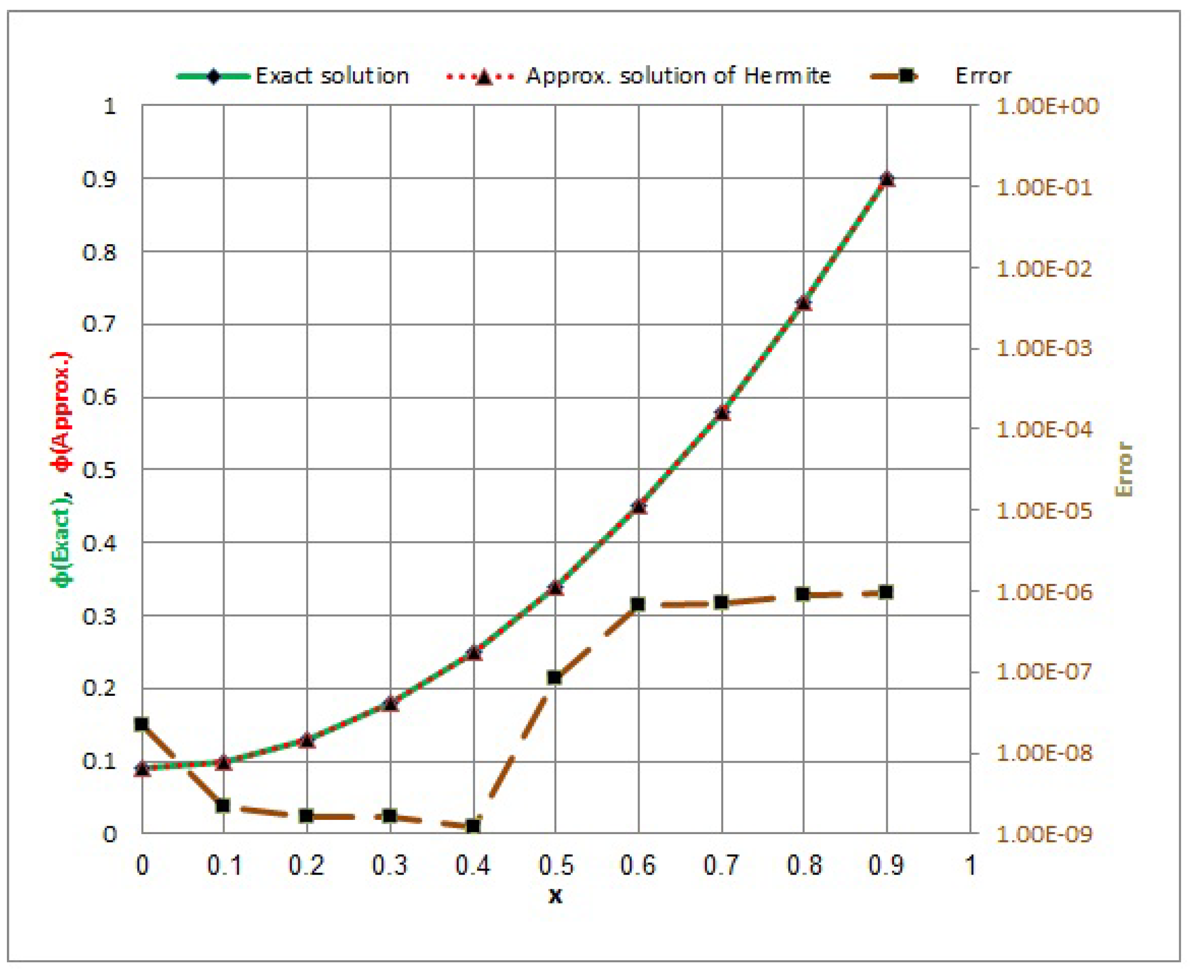
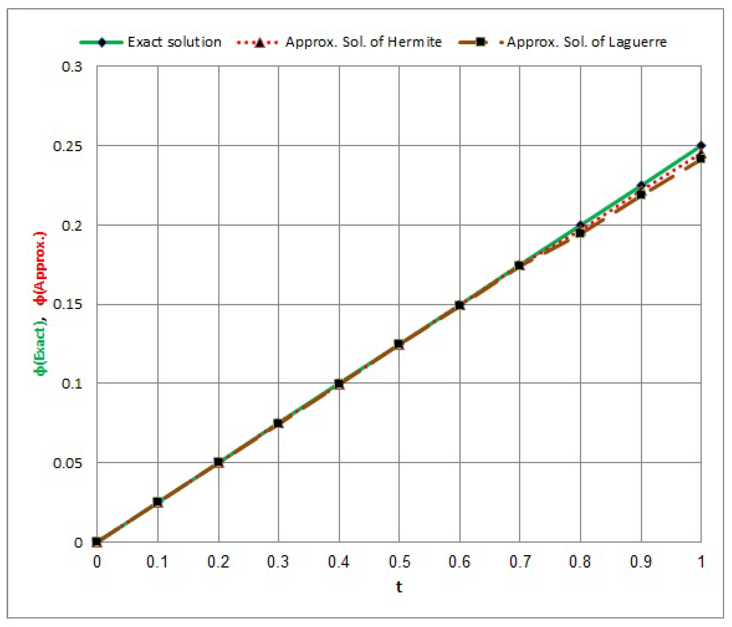
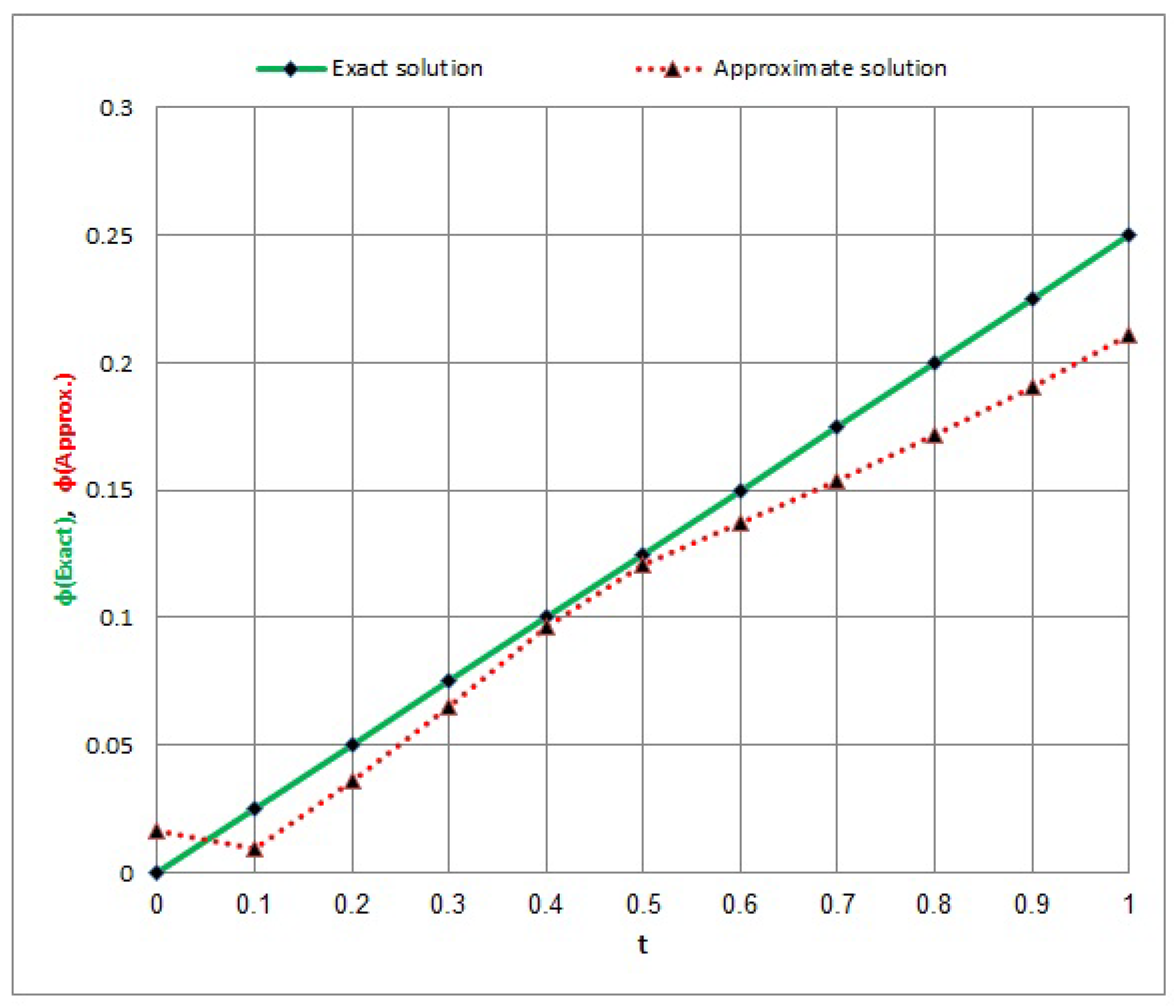
• From Example 1, for the quadratic integral equation Equation (27) in Table 1 and Figure 1 and Figure 2, the max. value error of the collocation method via Hermite polynomials is $(9.236\times {10}^{-7})$ at $t\in [0,0.6]$, while the max. value error of the collocation method via Laguerre polynomials is $\left(0.000006114\right)$ at $x=0.9$. In addition, the error of the collocation method via Laguerre and Hermite polynomials is decreasing at $x\in [0,0.4]$ and increasing at $x\in (0.4,0.9]$.
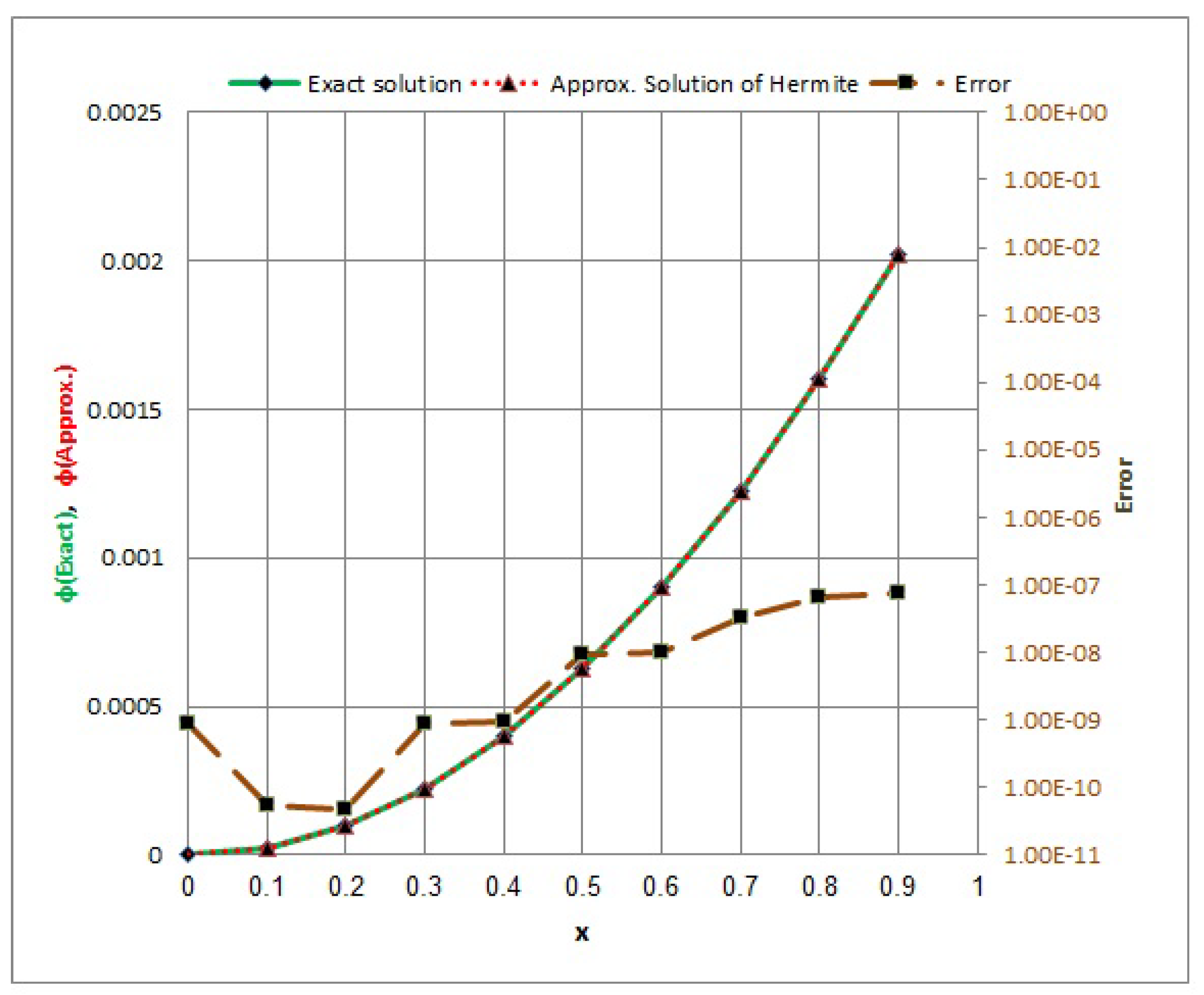
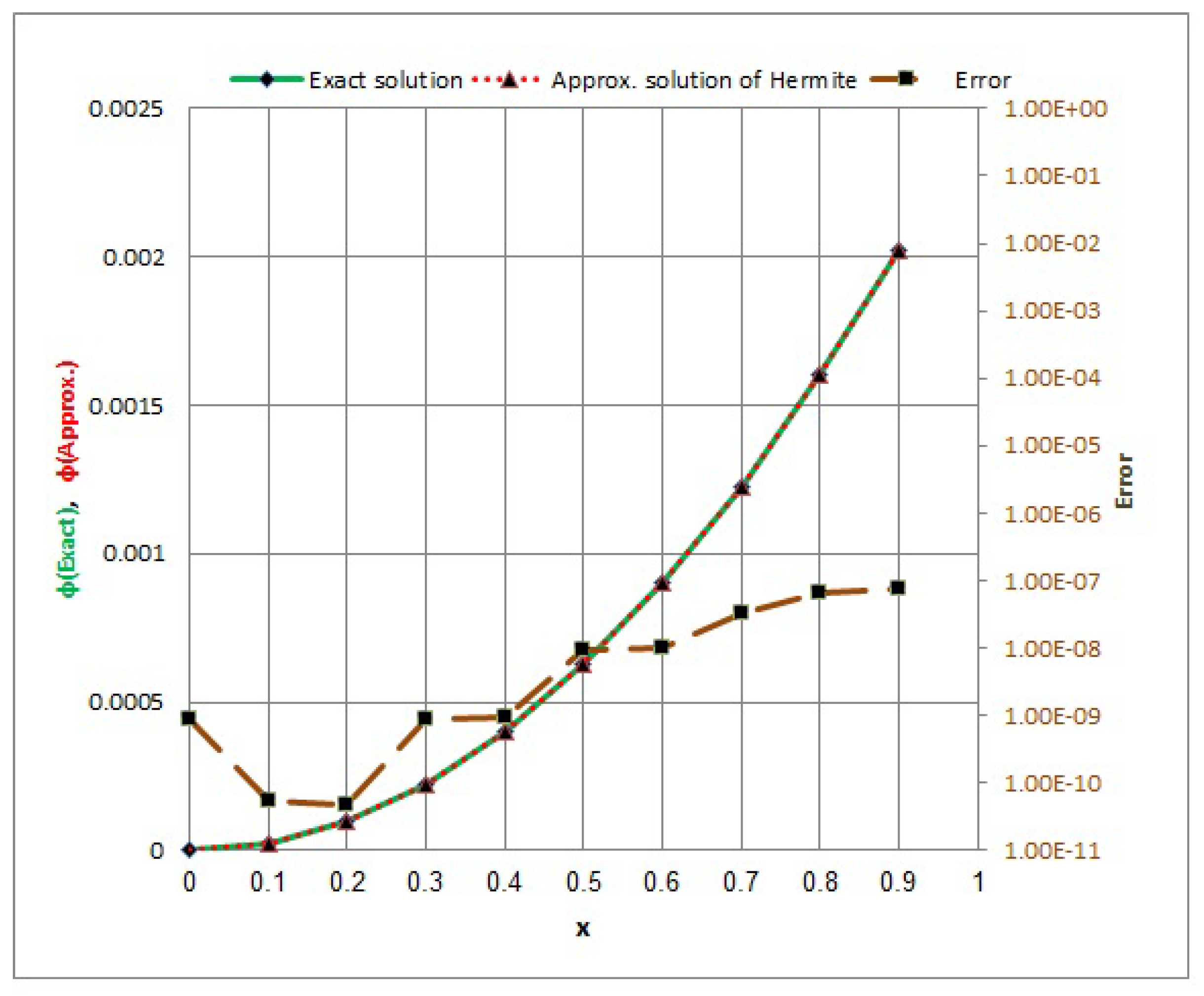
• In Example 2, for Equation (28) in Table 2 and Figure 3 and Figure 4, the max. value error of the collocation method via Hermite polynomials is $(7.412\times {10}^{-7})$ at $t\in [0,0.1]$, while the max. value error of the collocation method via Laguerre polynomials is $(9.058\times {10}^{-7})$. In addition, the error of the collocation method via Hermite polynomials is decreasing at $x\in [0,0.2]$ and increasing at $x\in (0.2,0.9]$, while the error of the collocation method via Laguerre polynomials is decreasing at $x\in [0,0.1]$ and increasing at $x\in (0.1,0.9]$.
• In Example 3, for Equation (29) of the second kind at $0\le t\le 0.01$ in Table 3 and Figure 5 and Figure 6, the max. value error of collocation method via Hermite polynomials is $(8.21\times {10}^{-19})$, while the max. value error of the collocation method via Laguerre polynomials is $(8.99\times {10}^{-18})$. The errors of the collocation methods via Laguerre and Hermite polynomials increase if the position x increases, and vice versa.
• From Examples 1–3, we notice that the numerical solution quickly converges to the exact solution when the variable t converges to 0. When the variable x takes the value $x=0.9$, we obtain a maximum value of the error; conversely, we find a minimum value of the error at $x=0$.
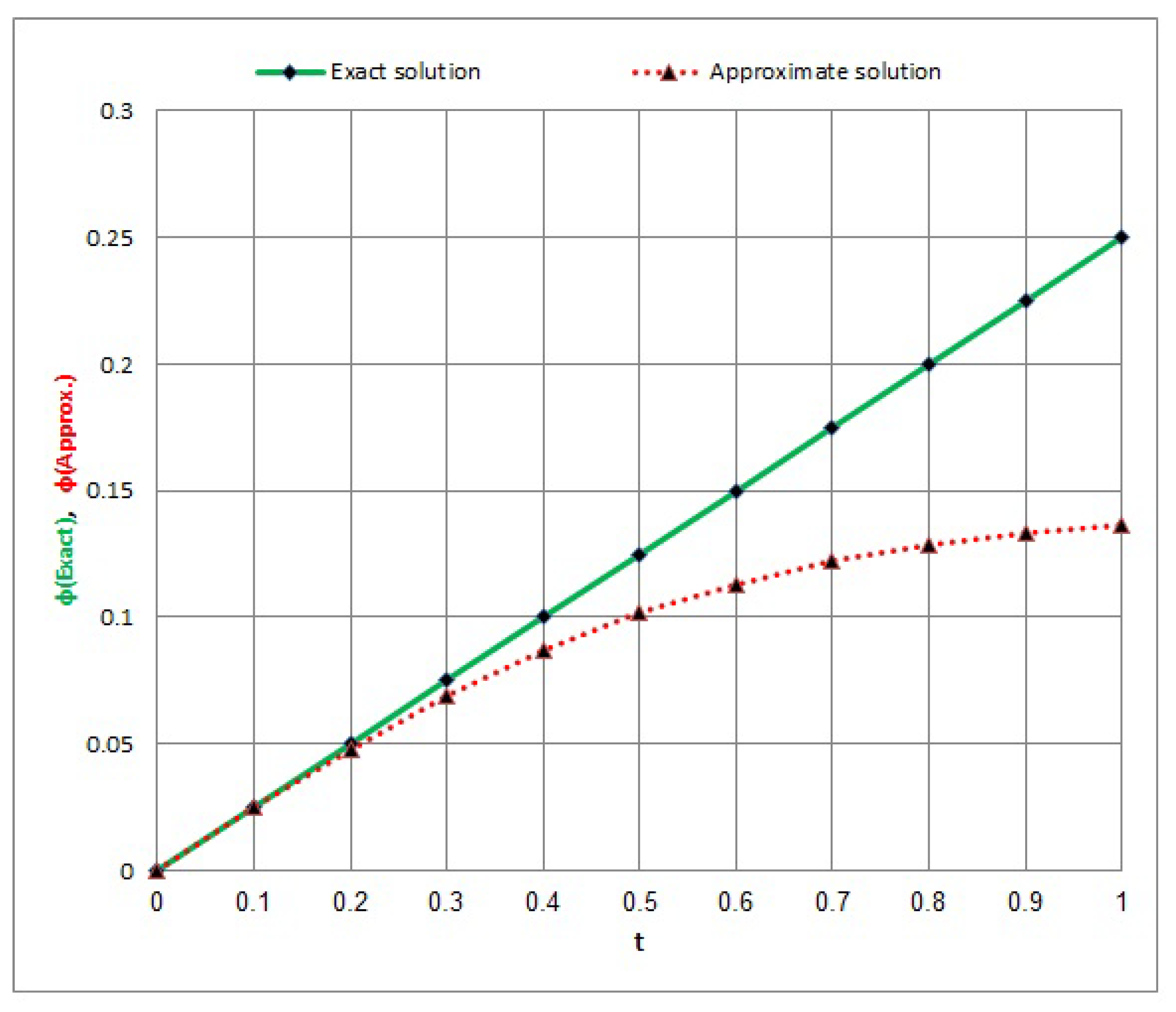
• In Example 4, we discussed Equation (30), which was discussed previously in [36]. We can see from Table 4 and Table 5, and Figure 7, Figure 8, Figure 9 and Figure 10 that the method studied in this article is more accurate in terms of results and better in providing a numerical solution closer to the exact solution.

7.2. Conclusions

Based on the results of this work, we can establish the following:

• In this research, a quadratic integral equation is discussed in a general form, in the space $C\left(\right[0,T]\times [0,T\left]\right),T<1$, from which many special cases can be derived. These special cases are considered important in application in many different fields.
• If in Equation (1), we let $E_2=1$, we have a nonlinear integral equation

  $$\mu \mathrm{\Phi }(x,t)=g(x,t)+E_1\left(x,t,{\int }_0^{t}f(x,\tau )\mathrm{\Phi }(x,\tau )\mathrm{d}\tau \right).$$

  (31)
  The above equation also has many applications in different fields.
• It is noted that the squaring method, which depends on dividing one of the variables into distances that may be equal or unequal, directly helps transform the quadratic integral equation in two variables into an algebraic system of quadratic integral equations in one variable.
• Combining the collocation method and orthogonal polynomials enables researchers to obtain more accurate and less error-prone solutions compared to other methods.

8. Future Work

The authors will consider the solution of the principal equation of this paper in two-dimensional problem with phase-lag in time:

$$\begin{array}{cc}\hfill \mu \mathrm{\Phi }(x,t+\delta t)=g(x,t+\delta t)& +E_1\left(x,t+\delta t,{\int }_0^{t+\delta t}f(x,\tau )\mathrm{\Phi }(x,\tau )\mathrm{d}\tau \right)\hfill \\ \hfill & \times E_2\left(x,t+\delta t,{\int }_0^{x}k(y,t+\delta t)\mathrm{\Phi }(y,t+\delta t)\mathrm{d}y\right),0<\delta t<1.\hfill \end{array}$$

References

1. Alhazmi, S.E.A. New Model for Solving Mixed Integral Equation of the First Kind with Generalized Potential Kernel. J. Math. Res. 2017, 9, 18–29. [Google Scholar] [CrossRef]
2. Ghiat, M.; Tair, B.; Ghuebbai, H.; Kamouche, S. Block-by-block method for solving non-linear Volterra integral equation of the first kind. Comp. Appl. Math. 2023, 42, 42–67. [Google Scholar] [CrossRef]
3. Gong, W.; Li, B.; Yang, H. Optimal Control in a Bounded Domain for Wave Propagating in the Whole Space: Coupling Through Boundary Integral Equations. J. Sci. Comput. 2022, 92, 91. [Google Scholar] [CrossRef]
4. Jaabar, S.H.; Hussain, A.H. Solving Volterra integral equation by using a new transformation. J. Interdiscip. Math. 2021, 24, 735–741. [Google Scholar] [CrossRef]
5. Matoog, R.T.; Abdou, M.A.; Abdel-Aty, M.A. New algorithms for solving nonlinear mixed integral equations. AIMS Math. 2023, 8, 27488–27512. [Google Scholar] [CrossRef]
6. Ma, Z.; Huang, C. Fractional Collocation Method for Third-Kind Volterra Integral Equations with Nonsmooth Solutions. J. Sci. Comput. 2023, 95, 26. [Google Scholar] [CrossRef]
7. Micula, S. On some iterative numerical methods for a Volterra functional integral equation of the second kind. J. Fixed Point Theory Appl. 2017, 19, 1815–1824. [Google Scholar] [CrossRef]
8. Micula, S. An iterative numerical method for Fredholm–Volterra integral equations of the second kind. Appl. Math. Comput. 2015, 270, 935–942. [Google Scholar] [CrossRef]
9. Sarkar, N.; Sen, M.; Saha, D. Solution of non linear Fredholm integral equation involving constant delay by BEM with piecewise linear approximation. J. Interdiscip. Math. 2020, 23, 537–544. [Google Scholar] [CrossRef]
10. Fatahi, H.; Saberi–Nadjafi, J.; Shivanian, E. A new spectral meshless radial point interpolation(SMRPI) method for the two–dimensional Fredholm integral equations on general domains with error analysis. J. Comput. Appl. Math. 2016, 294, 196–209. [Google Scholar] [CrossRef]
11. Noeiaghdam, S.; Dreglea, A.; He, J.; Avazzadeh, Z.; Suleman, M.; Fariborzi Araghi, M.A.; Sidorov, D.N.; Sidorov, N. Error estimation of the homotopy perturbation method to solve second kind Volterra integral equations with piecewise smooth kernels. Application of the CADNA library. Symmetry 2020, 12, 1730. [Google Scholar] [CrossRef]
12. Jaan, A.R. Solution of nonlinear mixed integral equation via collocation method basing on orthogonal polynomials. Heliyon 2022, 8, e11827. [Google Scholar] [CrossRef]
13. Abusalim, S.A.; Abdou, M.A.; Nasr, M.E.; Abdel–Aty, M.A. An Algorithm for the Solution of Nonlinear Volterra–Fredholm Integral Equations with a Singular Kernel. Fractal Fract 2023, 7, 730. [Google Scholar] [CrossRef]
14. Abdel–Aty, M.A.; Abdou, M.A. Analytical and Numerical Discussion for the Phase-Lag Volterra-Fredholm Integral Equation with Singular Kernel. J. Appl. Anal. Comput. 2023, 13, 3203–3220. [Google Scholar] [CrossRef] [PubMed]
15. Abusalim, S.A.; Abdou, M.A.; Abdel–Aty, M.A.; Nasr, M.E. Hybrid Functions Approach via Nonlinear Integral Equations with Symmetric and Nonsymmetrical Kernel in Two Dimensions. Symmetry 2023, 15, 1408. [Google Scholar] [CrossRef]
16. Adibi, H.; Shamooshaky, M.; Assar, P. CAS wavelet method for the numerical solution of boundary integral equations with logarithmic singular kernels. Int. J. Math. Model. Comput. 2014, 4, 377–387. [Google Scholar]
17. Abdel–Aty, M.A.; Abdou, M.A.; Soliman, A.A. Solvability of quadratic integral equations with singular kernel. J. Contemp. Math. Anal. 2022, 57, 12–25. [Google Scholar] [CrossRef]
18. Mirzaee, F.; Hoseini, S.F. Application of Fibonacci collocation method for solving Volterra–Fredholm integral equations. Appl. Math. Comput. 2016, 273, 637–644. [Google Scholar] [CrossRef]
19. Hesameddini, E.; Shahbazi, M. Solving system of Volterra–Fredholm integral equations with Bernstein polynomials and hybrid Bernstein Block-Pulse functions. J. Comput. Appl. Math. 2017, 315, 182–194. [Google Scholar] [CrossRef]
20. Alhazmi, S.E.A. Certain results associated with mixed integral equations and their comparison via numerical methods. J. Umm Al-Qura Univ. Appl. Sci. 2023, 9, 57–66. [Google Scholar] [CrossRef]
21. Mirzaee, F.; Hadadiyan, E. Numerical solution of linear Fredholm integral equations via two–dimensional modification of hat functions. Appl. Math. Comput. 2015, 250, 805–816. [Google Scholar] [CrossRef]
22. Bazm, S. Bernoulli polynomials for the numerical solution of some classes of linear and nonlinear integral equations. J. Comput. Appl. Math. 2015, 275, 44–60. [Google Scholar] [CrossRef]
23. Mirzaee, F.; Samadyar, N. On the numerical solution of stochastic quadratic integral equations via operational matrix method. Math. Methods Appl. Sci. 2018, 41, 4465–4479. [Google Scholar] [CrossRef]
24. Benkerrouche, A.; Souid, M.S.; Stamov, G.; Stamova, I. On the solutions of a quadratic integral equation of the Urysohn type of fractional variable order. Entropy 2022, 24, 886. [Google Scholar] [CrossRef]
25. Heydari, M.H. A computational method for a class of systems of nonlinear variable-order fractional quadratic integral equations. Appl. Numer. Math. 2020, 153, 164–178. [Google Scholar] [CrossRef]
26. Metwali, M. On some properties of Riemann–Liouville fractional operator in Orlicz spaces and applications to quadratic integral equations. Filomat 2022, 36, 6009–6020. [Google Scholar] [CrossRef]
27. Abdou, M.A.; Soliman, A.A.; Abdel-Aty, M.A. Analytical results for quadratic integral equations with phase-lag term. J. Appl. Anal. Comput. 2020, 10, 1588–1598. [Google Scholar] [CrossRef]
28. El–Sayed, A.M.A.; Hashem, H.H.G.; Omar, Y.M.Y. Positive continuous solution of a quadratic integral equation of fractional orders. Math. Sci. Lett. 2013, 2, 19–27. [Google Scholar] [CrossRef]
29. Abdel–Aty, M.A.; Abdou, M.A. Analytical and numerical discussion for the quadratic integral equations. Filomat 2023, 37, 8095–8111. [Google Scholar] [CrossRef]
30. Mirzaee, F.; Hadadiyan, E. Application of modified hat functions for solving nonlinear quadratic integral equations. Iran J. Numer. Anal. Opt. 2016, 6, 65–84. [Google Scholar] [CrossRef]
31. Arab, R.; Allahyari, R. Shole Haghighi, A. Existence of solutions of infinite systems of integral equations in two variables via measure of noncompactness. Appl. Math. Comput. 2014, 246, 283–291. [Google Scholar] [CrossRef]
32. Basseem, M.; Alalyani, A. On the solution of quadratic nonlinear integral Equation with different singular kernels. Math. Probl. Eng. 2020, 2020, 7856207. [Google Scholar] [CrossRef]
33. Banaś, J.; Jleli, M.; Mursaleen, M.; Samet, B.; Vetro, C. (Eds.) Advances in Nonlinear Analysis via the Concept of Measure of Noncompactness; Springer Nature: Singapore, 2017. [Google Scholar] [CrossRef]
34. Pourhadi, E.; Saadati, R.; Nieto, J.J. On the attractivity of the solutions of a problem involving Hilfer fractional derivative via the measure of noncompactness. Fixed Point Theory 2023, 24, 343–366. [Google Scholar] [CrossRef]
35. Delves, L.M.; Mohamed, J.L. Computational Methods for Integral Equations; Cambridge University Press: New York, NY, USA, 1988. [Google Scholar]
36. Mishra, L.N.; Pathak, V.K.; Baleanu, D. Approximation of solutions for nonlinear functional integral equations. AIMS Math. 2022, 7, 17486–17506. [Google Scholar] [CrossRef]
Figure 1. Exact solution, approximate solution, and absolute error of Hermite Polys. For 0 t 0.6 .
Axioms 13 00621 g001
Figure 2. Exact solution, approximate solution, and absolute error of Laguerre Polys. For 0 t 0.6 .
Axioms 13 00621 g002
Figure 3. Exact solution, approximate solution, and absolute error of Hermite Polys. For 0 t 0.1 .
Axioms 13 00621 g003
Figure 4. Exact solution, approximate solution, and absolute error of Laguerre Polys. For 0 t 0.1 .
Axioms 13 00621 g004
Figure 5. Exact solution, approximate solution, and absolute error of Hermite Polys. For 0 t 0.01 .
Axioms 13 00621 g005
Figure 6. Exact solution, approximate solution, and absolute error of Laguerre Polys. For 0 t 0.01 .
Axioms 13 00621 g006
Figure 7. Approximate and exact solutions of Hermite and Laguerre Polys for Φ 1 ( t ) .
Axioms 13 00621 g007
Figure 8. Approximate solution and exact solution for Φ 1 ( t ) of [36].
Axioms 13 00621 g008
Figure 9. Approximate and exact solutions of Hermite and Laguerre Polys for Φ 2 ( t ) .
Axioms 13 00621 g009
Figure 10. Approximate solution and exact solution for Φ 2 ( t ) of [36].
Axioms 13 00621 g010