Systematic Review

A Systematic Overview of Fuzzy-Random Option Pricing in Discrete Time and Fuzzy-Random Binomial Extension Sensitive Interest Rate Pricing

by
Jorge de Andrés-Sánchez
Social and Business Research Lab, Universitat Rovira i Virgili, Campus de Bellissens, 43204 Reus, Spain
Axioms 2025, 14(1), 52; https://doi.org/10.3390/axioms14010052
Submission received: 17 December 2024 / Revised: 2 January 2025 / Accepted: 7 January 2025 / Published: 10 January 2025
(This article belongs to the Special Issue New Perspectives in Fuzzy Sets and Their Applications, 2nd Edition)

Abstract

:
Since the early 2000s, fuzzy mathematics has fostered a stream of research on the financial valuation of assets incorporating optionality. This paper makes two contributions to this field. First, it conducts a bibliographical analysis of contributions from fuzzy set theory to option pricing, focusing on fuzzy-random option pricing (FROP) and its applications in binomial and trinomial lattice approaches. Second, it extends the FROP to yield curve modeling within a binomial framework. The bibliographical analysis followed the PRISMA guidelines and was conducted via the SCOPUS and WoS databases. We present a structured review of papers on FROP in discrete time (FROPDT), identifying the principal papers and outlets. The findings reveal that this focus has been applied to price options on stocks, stock indices, and real options. However, the exploration of its application to the term structure of interest-sensitive interest rate assets is very rare. To address this gap, we develop a fuzzy-random extension of the Ho–Lee term structure model, applying it to the European interbank market and price caplet options.

1. Introduction

1.1. Preliminary Considerations

Although the existence of option and future agreements can be traced back to ancient civilizations, the first serious attempts to develop mathematical option pricing date to the late 19th and early 20th centuries, with authors such as Bachelier and Bronzin [1,2]. Surprisingly, developments in the valuation of derivative assets did not attract academic interest until the mid-20th century, when authors such as Samuelson revisited the works of Bachelier and Bronzin [2,3].
It is commonly agreed that contributions by Black and Scholes [3] and Merton [4] in 1973, specifically the formulas used to price European options, are the keystone of option pricing theory [5]. We refer to these formulas as the BSM. The groundwork provided by the BSM has been widely extended, not only to the narrow field of financial options but also to the value of financial and real assets. Of course, derivatives such as warrants or convertible bonds can be naturally priced as options, but the BSM framework has also allowed the development of formulas for new option types such as so-called “exotic” and new derivatives such as credit default swaps or catastrophe derivatives [5]. In fact, ref. [3] proposed using the BSM to price options and warrants but also corporate liabilities, and [4] did so to measure firms’ credit risk. Similarly, the use of option pricing models to assess decisions on real assets and capital budgeting problems, the so-called real option theory [5], has received much attention since the early 1990s. Since that decade, more complex option pricing models, such as stochastic volatility models [2,5], have been developed.
The BSM approach has been particularly influential in modeling yield curves. A key goal of this research area is to establish a mathematical framework for pricing interest-sensitive financial instruments. As outlined in [6], models can be categorized into those with time-independent parameters [7,8,9,10] and those with time-dependent parameters [11,12,13]. While the first type of yield curve model dates from the late 1970s to the mid-1980s, time-dependent models were subsequently developed between the late 1980s and the mid-1990s [6].
Nondependent time models are unable to accurately fit the actual shape of the temporal structure of interest rates. The limitation of these models lies in their construction. They assume that the dynamics of interest rates are known and then derive zero-coupon bond prices using arbitrage arguments. While these models offer valuable insights into the temporal structure of interest rates, they fail to accurately reflect the observed shapes of yield curves, making them ineffective for pricing interest-sensitive instruments [6]. Conversely, time-dependent models treat zero-coupon bond prices as given parameters and use arbitrage arguments to model the dynamics of short-term rates. Owing to their design, this approach enables them to accurately capture the shapes of yield curves [6].
Although continuous-time option pricing models such as the BSM provide a reliable framework to price contingent assets, they are neither flexible enough to price American options or path-dependent options nor to model complex and poorly structured real options [14,15]. In this context, the binomial option approach initially proposed by Cox, Ross, and Rubinstein [16] and Rendleman and Bartter [17] has also attracted much attention from practitioners and academicians [15]. Binomial options have been used to price European options, American options, exotic options [15], and, of course, fixed-income assets and the term structure of interest rates [18,19].
Financial trades are conducted with varying levels of information and knowledge. Risk entails that the probabilities of different potential outcomes for an event can be quantified. While stochastic mathematics has been effectively used to model option pricing, the parameters governing the probabilistic price movements of the underlying asset may not be entirely precise. This uncertainty can arise from factors such as vagueness or ambiguity [20].
Since the beginning of the 21st century, fuzzy set theory (FST) has provided options for pricing reliable mathematical tools for modeling nonprobabilistic uncertainty, such as fuzzy measures, fuzzy numbers, or fuzzy regression [21]. Although probability theory offers a robust analytical foundation, incorporating fuzzy tools can improve its outcomes by accounting for additional sources of uncertainty, such as imprecision or ambiguity [20,21]. In the context of fuzzy set theory (FST) applied to option pricing (FOP), four distinct streams can be identified [21]:
  • Fuzzy random option pricing (FROP). Broadly, it is based on traditional option pricing models, with the uncertainty in various parameters, such as volatility, the observed price of the underlying asset, or discount rates, being represented via fuzzy numbers (FNs) [20].
  • Option pricing with Sugeno’s fuzzy measures and Choquet’s integral. By integrating these analytical tools with traditional option pricing formulas, this approach enables the modeling of Knightian uncertainty. It addresses market friction issues such as liquidity shortages and the risk of issuer defaults [22].
  • The fuzzy pay-off method [23] is centered around real option pricing. It is undoubtedly one of the most modern approaches in fuzzy option pricing, as the first works date back to the late 2000s.
  • Nonparametric option pricing. Contributions in this stream leverage tools such as fuzzy neural networks and fuzzy expert systems for option pricing, capitalizing on their ability to serve as universal function approximators [21].

1.2. Research Objectives

This paper has two aims. The first objective is to describe the results of a systematic search of the literature on FROP until July 2024 in the WoS and SCOPUS databases, focusing on discrete time developments. We label this stream of research fuzzy-random option pricing in discrete time (FROPDT). The review strictly considers those studies that use binomial and trinomial lattices. This analysis is relevant to motivate our extension of fuzzy-binomial lattices to model the temporal structure of interest rates and to outline further research in the discussion section.
The second objective is driven by the fact that contributions in FROP and FROPDT, specifically related to fixed-income instrument pricing, are scarce. In continuous time, ref. [24] extends Vasicek’s nonarbitrage model of term structures of interest rates [7] to incorporate fuzzy volatility and mean-reverting parameters, and [25] extends Jamshidian’s model of option pricing on zero-coupon bonds [26]. In discrete time, ref. [27] develops a binomial model of the term structure of interest rates to value game option bonds when estimates of bond prices and interest rate volatility come via FNs.
This paper develops a fuzzy-random extension of the model of yield rates [11] to price interest rate derivatives such as caplets. This extension employs a binomial lattice and assumes fuzzy volatility of short-term rates, which is estimated via the methodology [28]. This focus allows the construction of membership functions of uncertain variables from observed data and is a coherent probability-possibility transformation [29]. We provide an empirical application of our fuzzy extension to Euribor monthly rates.
Furthermore, although the variables derived from market data (short-term spot rates and the prices of interest rate derivatives) are not triangular FNs, we explore the suitability of their triangular approximation, given the intriguing properties of this type of FN [30].

2. A Systematic Bibliographical Revision of Fuzzy-Random Option Pricing in Discrete Time

2.1. Materials and Methods

The bibliographical analysis in this paper was conducted following the PRISMA guidelines [31] and is registered in the Open Science Framework (https://doi.org/10.17605/OSF.IO/4RJWH). These guidelines require specifying the strategies used to identify the works for review, the databases consulted, the inclusion criteria, and the examination procedures. The subsequent step involves detailing the process of compiling bibliometric references. Finally, the study qualitatively and quantitatively analyzes the contributions of FROPDT and examines the temporal evolution of research in this field. The PRISMA checklist can be consulted in the Supplementary Materials of the paper (https://www.mdpi.com/article/10.3390/axioms14010052/s1).
Only documents published in journals and book chapters until 31 October 2024 were eligible. We did not review gray literature such as working papers, conference papers, or papers in digital repositories because these works, with the help of a peer-review process, are usually disseminated subsequently as articles or book chapters. We only took into account papers published in English. When the topic is not so wide, as is the case for fuzzy stochastic option pricing, especially FROPDT, it is preferable to combine more than one bibliographical database [32]; thus, we combined SCOPUS and WoS.
The exploration of the databases was performed over the titles, abstracts, and keywords using the following search: (“option pricing”) AND (“fuzzy sets” OR “fuzzy mathematics” OR “fuzzy numbers”). Figure 1 illustrates the methodology used in our study. A total of 92 documents were retrieved from SCOPUS, and 185 were retrieved from WoS. After removing duplicates, we reviewed the title, abstract, keywords, and introduction of the remaining documents. When needed, the full text was examined to confirm the paper’s focus on FROP using binomial and trinomial lattices. This process ultimately identified 37 relevant documents related to FROPDT, as summarized in Table 1.
We found 27 documents common to both databases: four were provided exclusively by WoS, and six were provided by SCOPUS. By considering these 37 contributions, we then calculated Meyer’s index [33], which quantifies the coverage level attributable to each consulted database and the overlap degree, which sizes the database redundancy.
When J papers are reviewed, Meyer’s index for the ith database, M e y e r i , (i = 1,2, …, n) is as follows:
M e y e r i = j = 1 J w i , j J ,
where w i , j is the weight of the contribution that database i has in paper j. If database i includes article j, w i , j = 1 / n j , where n j n and n j is the number of databases that include paper j. If database i does not include the jth contribution, w i , j = 0 . Thus, Meyer’s index for WoS is (4 + 27 × 0.5)/37 = 47.30%, and for SCOPUS, it is (6 + 27 × 0.5)/37 = 52.70%.
The degree of overlap of database i with database h, O v e r l a p i , h , is obtained as follows:
O v e r l a p i , h = n i , h n i ,
where n i , h is the number of papers that are contained in both databases i and h , and n i is the number of works contained in the ith database. Therefore, the overlap degree of WoS is 27/(27 + 4) = 87.10%, and that of SCOPUS is 27/(27 + 6) = 81.82%.
Figure 1. PRISMA guidelines followed to choose papers on fuzzy-random option pricing and fuzzy-binomial option pricing papers to review. Source: based on [31].
Axioms 14 00052 g001
Table 1. Summary of contributions by fuzzy-random option pricing with binomial and trinomial lattices.
ReferenceYearMoves CalibrationUncertain
Parameters
Option TypeShape of the Fuzzy Quantities
Yoshida [34]2003Cox et al. [16]MovesAmerican styleTFNs
Muzzioli and Torricelli [35]2004Up and down moves may be independent and following Cox et al. [16]MovesApplication to stock option markets/European styleTFNs
Lee et al. [36]2005Cox et al. [16]MovesStock market application/European styleTriangular and symmetric FNs
Buckley and Eslami [37]2007Moves are calibrated from a symmetric ± a%Subjacent asset price, strike price, discount rate, and movesEuropean styleTFNs
Muzzioli and Reynaerts [38]2007Moves are independentMovesEuropean styleTFNs
Buckley and Eslami [39]2008Moves are calibrated from a symmetric ± a%Initial asset price, strike price, interest rate, and movesEuropean styleTFNs
Muzzioli and Reynaerts [40]2008Cox et al. [16]MovesAmerican styleTrapezoidal/TFNs
Liao and Ho [41]2010Moves may be independent and following Cox et al. [16]Initial asset price and movesReal options/capital budgetingTFNs
Wang, Wang, and Watada [42]2010Cox et al. [16]Cash-flows and strike priceReal options/capital budgetingTFNs
Zmeskal [43]2010Cox et al. [16], but the use of alternatives such as Rendleman and Bartter [17] is suggestedInitial asset price, strike price, interest rate, and movesAmerican/Value of a companyTrFNs
Tolga, Kahraman, and Demircan [44]2010Trinomial moves are calibrated with [45]Present value of cash-flows. Moves and probabilities are crispReal options/capital budgetingTrFNs
Allenotor and Thulasiram [46]2011Trinomial moves are calibrated with [45]Present value of cash-flows. Moves and probabilities are crispReal options/capital budgetingTrFNs/and trapezoidal linguistic variables
Ho and Liao [47]2011Moves can be independently calibrated, but with Cox et al. [16]Strike price and movesReal options by taxonomyTFNs
Yu et al. [48]2011Cox et al. [16]MovesEuropeanTFNs
Elahi and Azziz [49]2012Moves may be independentPrice, strike price, and movesAsian financial optionsNot defined
Tolga, Tuysuz, and Kahraman [50]2013Trinomial moves are calibrated with [45]Present value of cash-flows. Moves and probabilities are crispReal options/capital budgetingTrFNs
Cruz-Aranda, Ortiz, and Cabrera-Llanos [51]2014Cox et al. [16]MovesReal options/capital budgetingTFNs
Muzzioli and de Baets [20]2016Review on fuzzy-random option pricingStock markets----
Anzilli and Facchinetti [52]2017Cox et al. [16]MovesReal options/life insurance guaranteesTFNs
Anzilli, Facchinetti, and Pirotti [53]2018Cox et al. [16]MovesLife insurance guaranteesAdaptive FNs
Xu, Liu, and Xu [54]2018Cox et al. [16]Recovery rate and movesVulnerable options of American styleTFNs
Zhang and Watada [55]2018Cox et al. [16]MovesAmerican options on stock indicesAdaptive FNs
D’Amato et al. [56]2019Moves are independently fittedMovesReal options/capital budgetingTFNs
Cruz-Aranda and Terán-Bustamente [57]2019Cox et al. [16]MovesReal options/capital budgetingTFNs
Meenakshi and Felbin [58]2019Moves are independently fittedInitial asset price, strike price, interest rate, and movesAmerican styleTrFNs
Shang et al. [59]2020Moves are independently fittedMovesReal options/capital budgetingParabolic FNs
Chrysafis and Papadopoulos [60]2021Cox et al. [16]Initial asset price, interest rate, and movesReal options/capital budgetingEmpirical FNs
Meenakshi and Kennedy [61]2021Moves are independently fittedInitial asset price, strike price, interest rate, and movesEuropean styleTrFNs
Meenakshi and Kennedy [62]2021Cox et al. [16]Initial asset price, strike price, interest rate, and movesAmerican styleOctogonal FNs
Wang, Wang, and Tang [63]2022Moves are independently fittedMovesFinancial optionsTrFNs
Zmeskal, Dluhošová, Gurný, and Kresta [64]2022Cox et al. [16]Initial asset price, strike price, interest rate, and movesReal options, multimodeTrFNs
Zmeškal, Dluhošová, Gurný, and Guo [27]2022Binomial lattice by [11]Bond spot prices and interest rate volatilitiesOptions on bond gamesAdaptive FNs
Andrés-Sánchez [21]2023Cox et al. [16]Initial asset price, strike price, interest rate, and movesEuropean styleTFNs
Ersen, Tas, and Ugurlu [65]2023Trinomial moves are calibrated with [45]Present value of cash-flows. Moves and probabilities are crispReal options/capital budgetingTrapezoidal/intuitionistic FNs
Zhang and Yin [66]2023Cox et al. [16]MovesReal options/capital budgetingSymmetric/TFNs
Agustina, Sumarti, and Sidarto [67]2024Binomial moves by Cox et al. [16] and trinomial moves by
Kamrad and Ritchken [66]
MovesEuropean StyleAdaptive FNs
Andrés-Sánchez [68]2024Cox et al. [16] and Rendleman and Bartter [17]MovesEuropean Style/Option on IndexesEmpirical intuitionistic FNs/triangular intuitionistic FNs

2.2. Analysis of the Content of the Reviewed Papers

Table 1 provides a summary of papers on FROPDT. The predominant approach involves the use of a binomial lattice, with 33 papers adopting this method. In contrast, only five contributions applied a trinomial lattice [44,46,50,65,67], and the first four contributions are linked to real options.
In FROPDT models, up (u) and down (d) multipliers are used as FNs. Most studies in this area have employed linear FNs. Specifically, 19 contribution model variables are triangular fuzzy numbers (TFNs), and 11 are trapezoidal fuzzy numbers (TrFNs). Less common alternatives include the use of fuzzy or intuitionistic FNs estimated from empirical data with coherent probability-possibility transformations [60,69] or some form of generalization of linear FNs [27,53,55,59,62,64].
In a trinomial setting, while only [67] introduces uncertainty in the moves, the [44,46,50,65] model moves and their probabilities are crisp parameters. Similarly, whereas [44] fuzzyifies the type of option by means of linguistic fuzzy variables and the price of the real asset as a TrFN, ref. [65] supposes that cash flows and yield rates of the investment project are quantified with intuitionistic TrFNs.
FROPDT provides two ways to fit fuzzy up and down multipliers u ( u ~ ) and d ( d ~ ) . The first method considers that the fuzzy multipliers are estimated independently by decision makers’ evaluations [35,38,41,48,56,58,59,61,62,63]. Therefore, these fuzzy multipliers are not linked. Alternatively, the decision maker may state a symmetric up/down move rate a ~ such that u ~ = 1 + a ~ and d ~ = 1 a ~ [37,39]. In this last approach, u ~ and d ~ are connected by rate a ~ . The alternative is to link the multipliers to the annual volatility of the subjacent asset, σ ~ , with the CRR model [16]. Therefore, u ~ = e σ ~ h , d ~ = e σ ~ h , and h represents the crisp periodicity of the jumps. This is the mainstream model in Table 1. In this case, u ~   and d ~ come directly from a quantification of σ ~ . Notably, ref. [69] conducted a comparison, assuming volatility estimated via an intuitionistic FN, of the convergence to prices provided by the BSM model by the Cox et al. [16] and Rendleman and Bartter [17] models, with results clearly favoring the latter.
An important consideration in fuzzy-binomial models is whether fuzzy uncertainty applies solely to the multipliers or extends to other parameters, such as the free discount rate or the initial price of the underlying asset. It is common to introduce fuzziness specifically in terms of the up and down moves, as seen in 17 contributions. However, some models also consider fuzziness in other parameters, including the strike price, with 20 papers addressing this broader approach. The specific parameters that are treated as fuzzy, in addition to the up and down factors, depend on the context in which FROPDT is applied. In this regard, we observe that FROPDT has been used to price European-style stock and index options (11 papers), American options (8 papers), real options (12 contributions), life insurance guarantees [52,53], and vulnerable options [58]. Notably, only one study has applied fuzzy options to interest-rate-sensitive instruments [27].

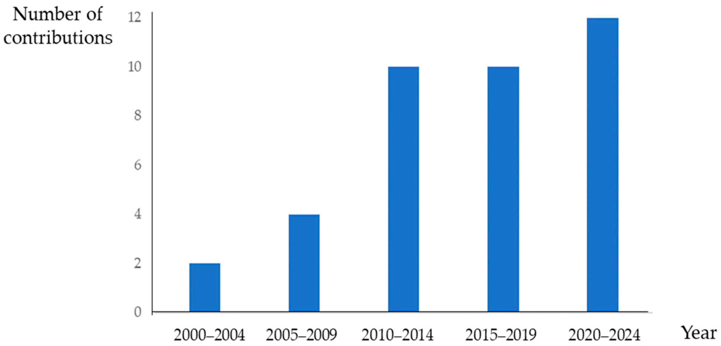
2.3. Quantitative Analysis of the Contributions of FROPDT

Figure 2 shows the evolution across the time of contributions to FROPDT since its inception. If we limit our review to journal papers and book chapters, that origin can be traced back to Yoshida’s work [34]. It can be observed that until 2010, FROPDT represented a niche within fuzzy mathematics that was not yet consolidated but showed a growing trend. From 2010 onward, contributions stabilized, with journal publications averaging at least 10 per five-year period over the following 15 years. That is, it is a small section within fuzzy mathematics, but it is solidly established.
Based on Table 1 and Figure 2, we can establish the following trends in FROPDT contributions, grouped by the following decades: from 2000 to 2009, from 2010 to 2019, and from 2020 onwards.
  • From 2000 to 2009, seven studies focused on analyzing algebraic issues related to the application of fuzzy arithmetic in the mathematics of option valuation [34,37,38,39,40]. Two studies involved empirical applications with market data [35,36].
  • From 2010 to 2019, among the 18 studies reviewed, a large number analyzed the application of FROPDT in real options valuation [41,42,44,45,46,50,52,53,56,57]. By definition, real options, which arise from specific investment projects, do not involve empirical applications with large datasets. During this decade, FROPDT applications emerged in other areas, such as business valuation [43], life insurance guarantees [52,53], and vulnerable options [54]. Only in [55] is there an extensive application using market data.
  • From 2020 onwards, the trend is similar to that of the previous decade. The application of FROPDT in real option pricing is an established topic [22,59,60,65,66]. There are studies addressing issues related to the implementation of option valuation using the binomial approach [61,62,63,67] and others exploring the valuation of options not analyzed in previous decades, such as bond games [27]. Only in [67,68] is there an empirical application using market data.
Table 2 presents the outlets for FROPDT. These outlets range from generalist soft computing journals, such as Expert Systems with Applications, the International Journal of Approximate Reasoning, and Information Sciences, to more specialized journals focused on fuzzy set theory, such as IEEE Transactions on Fuzzy Systems, and those with a broader operational research focus, such as the European Journal of Operational Research. Additionally, there are contributions in journals with other orientations, including finance (Contaduría y Administración and the Review of Quantitative Finance and Accounting), general economics (the Journal of Applied Economic Sciences and the Journal of Economic Dynamics & Control), and sector economics (Energy Policy and Land Use Policy).
Table 3 presents the most influential papers on FROPDT. The most cited paper [35] focuses on financial options and provides an empirical application using the DAX index, whereas the second [43], third [47], and sixth [41] most cited papers concentrate on real options. Among the top five most cited papers, three address the pricing of American options [34,40,43]. The seventh paper, ranked by citations in the SCOPUS database [36], is not indexed in WoS. This finding indicates that combining both the WoS and SCOPUS databases offers a more comprehensive exploration of the FROPDT literature. Additionally, Table 3 highlights two papers [20,21] that do not address a specific issue related to FROPDT but instead provide reviews contextualizing fuzzy logic’s contributions to option pricing.
Figure 3 shows the countries contributing the most to FROPDT. When authors are affiliated with institutions in multiple countries, we consider the country of the institution to which the corresponding author is affiliated. The country with the highest number of contributions is Italy, with seven contributions, followed by Taiwan (five contributions) and Turkey (four contributions). Additionally, up to nine other countries have contributed at least one paper to FROPDT.

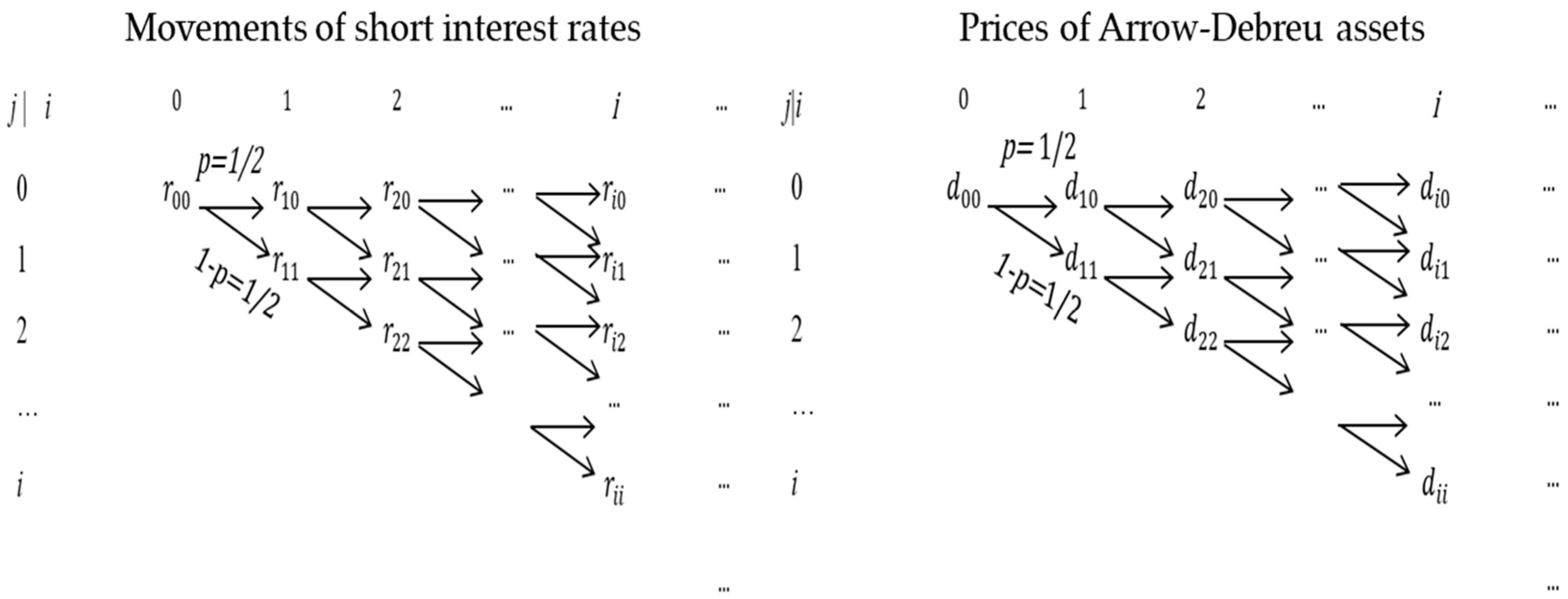
3. Binomial Lattice of the Term Structure of Interest Rates

3.1. Pricing Sensitive Interest-Rate Assets with a Binomial Lattice

A widely used method for pricing interest rate-sensitive contingent assets involves the use of binomial lattices to model the evolution of short-term rates [19]. These lattices offer reliable discrete-time approximations of standard single-factor continuous-time models based on Brownian motion for interest rates [18]. In our study, we focus on extending a recombinant binomial lattice, as illustrated in Figure 4, which underpins nonarbitrage term structure models such as those in [11,12]. In Figure 4, r i j represents the short discount rate during the ith period in the jth state. Thus, in the ith period, there are i + 1 realizations. As p, we symbolize the neutral-risk probability of a down variation in the interest rate. As in [18], we consider p = 1 2 . Given that the probabilities of increasing and decreasing variations are prefixed, to achieve a proper fit, it is essential to have states of short-term rates that align with the actual structure of interest rates while adhering to predefined risk-neutral probabilities and the assumed dynamics of the short-term interest rate.
Using the tree of interest rates, a corresponding tree of Arrow–Debreu asset prices can be derived, as illustrated in Figure 4. As d i j , we symbolize the actual value of an Arrow-Debreu that pays one monetary unit during the ith period in the jth state. By denoting the period of moves as h , d i j is decoupled into d i 1 , j 1 and d i 1 , j as follows:
d i j = 1 2 d i 1 , j 1 e r i 1 , j 1 · h + d i 1 , j e r i 1 , j · h .
In a complete market, the link between the price of a zero-coupon bond payable in i periods P i and d i j is as follows:
P i = j = 0 i d i j .
Following [18], this is as follows:
P i = j = 0 i d i 1 , j · e r i 1 , j · h .
Suppose an asset that only pays a cash flow in i·h years and that it depends on the short interest rate at the moment of payment. Therefore, in the jth state of nature, this discount rate is r i j , and the cash flow is denoted as c ( r i j ) 0 . The price, Π i , is as follows:
Π i = j = 0 i c ( r i j ) · d i j .

3.2. Pricing Sensitive Interest-Rate Assets with the Ho-Lee Model

Our analysis is confined to a linear constant variance Brownian process, the underlying stochastic process in continuous time that drives short-term rates [11]. Consequently, the short-term rate at any given instant t, r t ,   as follows:
d r t = θ t d t + σ d W t ,
where θ t is the slope of the interest rate at t, σ is the annual volatility, and d W t is a Gaussian random variable with a mean of 0 and a standard deviation of d t . The binomial version of (5) is the following [19]:
r i , j = r i 1 , j + θ i h σ h ,   a n d     r i , j + 1 = r i 1 , j + θ i h + σ h .
Note that r i , j can be rewritten in terms of r 0,0 and is a function of volatility. We suppose that this is the unique argument of the model (i.e., drifts are also parameters). Thus, r i , j is a function of σ , r i , j r i , j σ :
r i , j σ = r 0,0 + h k = 1 i θ k + 2 j i σ h .
Notice that the sign of the relationship between the rates and the volatility depends on i and j. It is easy to check in (6) that r i , j σ σ = 2 j i h . Therefore, r i , j σ decreases for j i 2 and increases otherwise. That is, the sparsity of the tree of interest rates increases as the volatility increases.
Taking into account that in j = 0, r i , 0 r i , 0 σ in such a way that:
r i , 0 σ = r 0,0 + h k = 1 i θ k i σ h .
Then, (6) can be written on the basis of the lower realization of the interest rate in the ith period r i , 0 (7):
r i , j σ = r i , 0 σ + 2 j σ h .
To price any contingent asset, we must calibrate the binomial movements of short-term rates using market data, which, within our analytical framework, are represented by the prices of zero-coupon bonds with maturities 1h, 2h, …, nh, that are denoted as P 1 , P 2 , , P n , and the volatility σ . The use of forward induction [18] allows for the estimation of the tree in Figure 4 via recursive fitting of d i , j from (1) and (8):
d i j σ = 1 2 d i 1 , j 1 σ e r i 1,0 σ + 2 j 1 σ h h + d i 1 , j σ e r i 1,0 σ + 2 j σ h h .
From (3) and (9),
P i + 1 = j = 0 i d i , j σ · e r i , 0 σ + 2 j σ h h .
Then,
r i , 0 σ = l n j = 0 i d i , j σ · e 2 j σ h h l n P i + 1 h .
Therefore, from (7), (8), and (10),
r i , j σ = l n j = 0 i d i , j σ · e 2 j σ h h l n P i + 1 h + 2 j σ h .
With this groundwork, the cash flows in (4) are a function of volatility, c ( r i j σ ) . Therefore, price is also a function of σ . Then,
Π i σ = j = 0 i c ( r i j σ ) · d i j σ .
In this extension of FROPDT, we price a caplet with a strike rate K, a notional of one monetary unit and maturity i · h . The rate K, in practice, is a simple interest rate. Thus, the short-term yield rate r i j σ in terms of a simple discount rate is ρ i j σ = e r i j σ h 1 h . The amount of the yield to be compensated at the end of the ith period per monetary unit of notional is c ( r i j σ ) = max ρ i j σ K , 0 · h . Equation (8) implies the following:
c ( r i j σ ) = max e ( r i , 0 σ + 2 j σ h ) h 1 h K , 0 · h · e ( r i , 0 σ + 2 j σ h ) h .

4. Binomial Lattices with an Additive Interest-Rate Model and Fuzzy Volatility

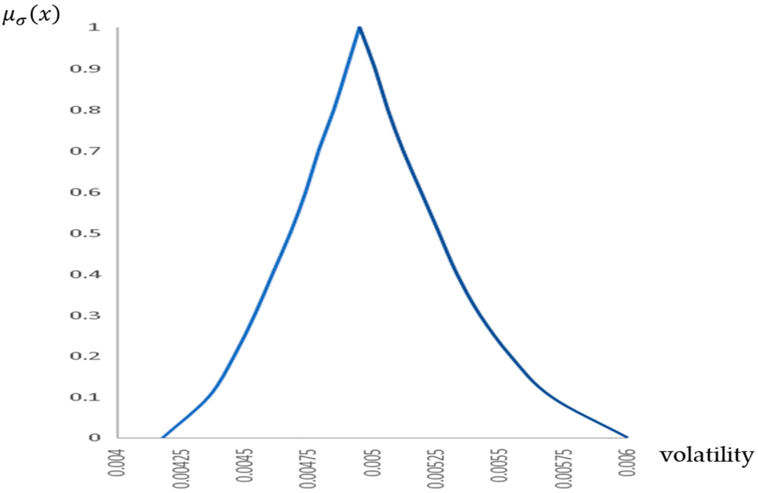
4.1. Fitting the Volatility of the Short-Term Interest Rates with Fuzzy Numbers

We extend the binomial approach to the yield curve, assuming that the short-term interest-rate dynamics described in Equations (5) and (8) are induced by fuzzy volatility σ ~ , with a membership function μ σ x . To apply the developments in Section 3, the α-cut representation of the annual volatility is more useful σ α = x | μ σ x α = σ α _ , σ α ¯   .
The assumption of fuzzy volatility is commonly agreed upon in FROPDT. In fact, as shown in Table 2, FROPDT is commonly developed through the consideration of σ ~ as a unique fuzzy parameter. Some examples of this approach include those of [35,36,48,53,56,63,66].
Table 1 shows that the literature often supposes volatility given by triangular, trapezoidal, or some kind of generalized linear FNs. However, in our empirical application, we induce an α-cut representation of σ α fitted by a probability-possibility transformation. We do so by following the methodology in [70] and refining it in [28] to construct FNs from statistical confidence intervals. This focus has been used in FROP [25,60,69,71]. In any case, the developments in this section can be performed with FNs of any shape.
From a set of observations of daily observations of short-term rates r 0,0 t , t = 1,2,…, n, whose first difference is Δ r 0,0 t , t = 1,2, …, n, we can measure the short-term interest rate volatility on a daily basis:
s d = t = 1 n Δ r 0,0 t t = 1 n Δ r 0,0 t n 2 n 1 .
A function linking the α-level of the FN and the statistical confidence intervals, f γ , α , where 2 f γ , α is the significance level associated with α , must also be stated. Following [28], f γ , α : 0,1 γ 2 , 0.5 , where γ ϵ ( 0,1 ) is the significance level whose confidence interval is considered a reference for the support of σ ~ (i.e., its 0-cut). A commonly used expression is the linear expression f γ , α = 1 2 γ 2 α + γ 2 [28], which is also used in this paper.
The fuzzy daily variance σ d ~ 2 and the annual variance σ ~ 2 are constructed by overlaying the statistical confidence intervals that we can build from s d 2 in (14). To do so, we state a general form for the α-cut of σ d ~ 2 as follows:
σ d 2 α = σ d 2 _ α , σ d 2 ¯ α = σ d 2 _ f γ , α , σ d 2 ¯ 1 f γ , α .
That is, σ d 2 _ f γ , α   and σ d 2 ¯ 1 f γ , α are the lower and upper extremes of the statistical confidence intervals for the variance of daily fluctuations of interest rates (14) at a significance level of 2 f γ , α . These extremes can be obtained, for example, using bootstrapping confidence intervals, asymptotic confidence intervals, or nonasymtotic confidence intervals [25]. If we use the nonasymptotic confidence intervals for σ d 2 α , by using (14) and (15), we find the following [28]:
σ d 2 α = σ d 2 _ α , σ d 2 ¯ α = ( n 1 ) · s d 2 χ n 1 ; f γ , α 2 , ( n 1 ) · s d 2 χ n 1 ; 1 f γ , α 2 ,
where χ a ; b 2 represents a chi-square distribution function with a degrees of freedom whose value is b . Therefore, the α-cuts of the fuzzy daily volatility of interest rates are, from (16), as follows:
σ d α = σ d 2 α = σ d _ α , σ d ¯ α = ( n 1 ) · s d 2 χ n 1 ; f γ , α 2 , ( n 1 ) · s d 2 χ n 1 ; 1 f γ , α 2 .
Therefore, the α-level sets of the annual volatility, σ α , are as follows:
σ α = σ α _ , σ α ¯     = 252 · σ d α = 252 · σ d _ α , 252 · σ d ¯ α .

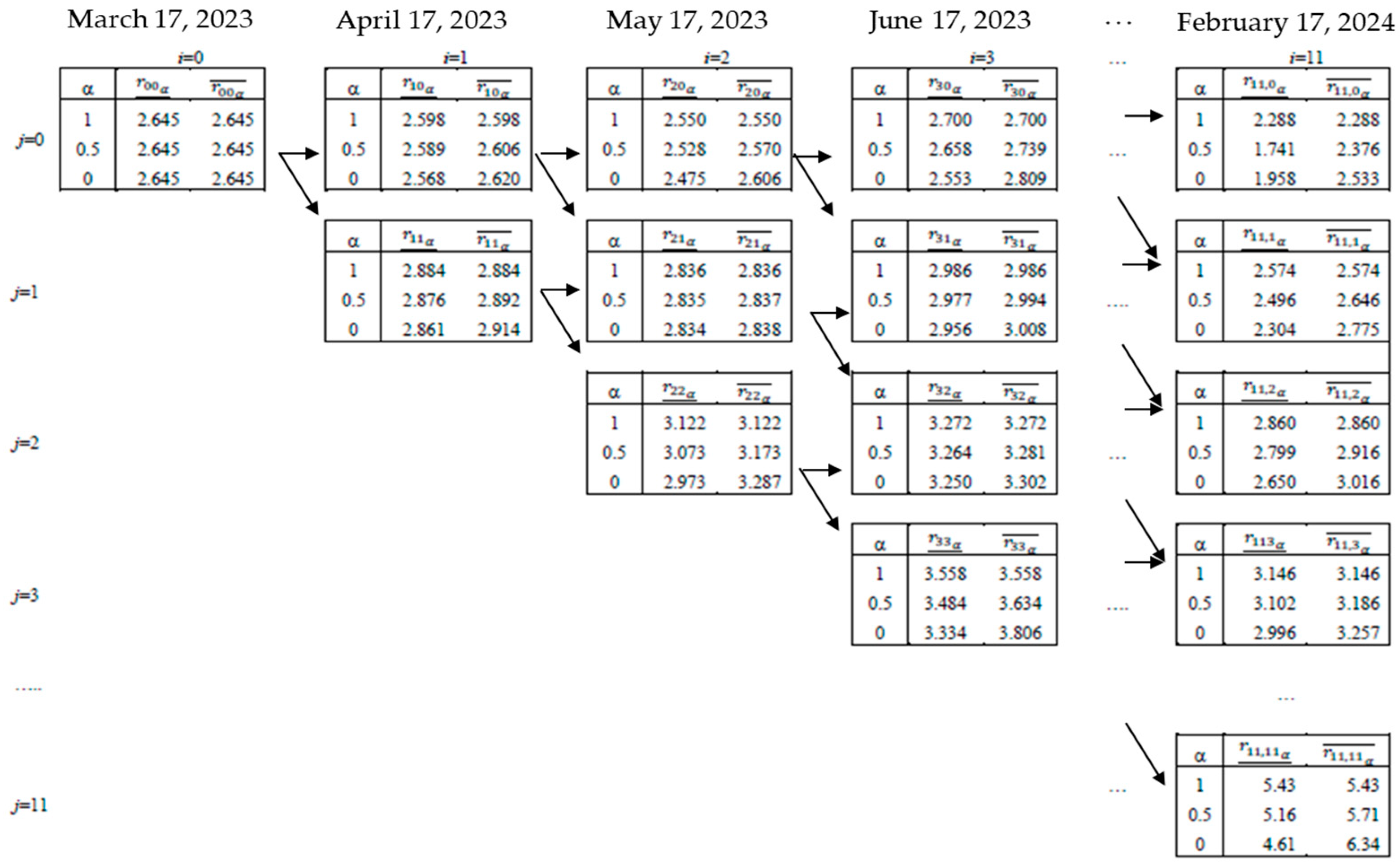
4.2. Pricing Interest-Rate Sensitivity Assets with a Fuzzy Ho and Lee Model of the Temporal Structure of Interest Rates

The interest rates of the three in Figure 4 are the interest rates from (6):
r ~ i , j = r 0,0 + h k = 1 i θ k + 2 j i σ ~ h .
To solve (6)–(12), we use the rules for the evaluation of functions of α-cuts [72]. To fit r ~ i , 0 in its α-cuts, it must be taken into account that higher volatilities induce more variability in binomial and, thus, more extreme states. Therefore, the lower state r i , 0 must decrease with volatility and the greater state r i , i must increase. In fact, (6) decreases in the ith period with σ for the state j in 0 ≤ j i 2 . Therefore, in this case, and via (11), the following is true:
r i , j α = r i , j α _ , r i , j α ¯ = r i , j σ α ¯ , r i , j σ α _   = l n j = 0 i d i , j σ α ¯ · e 2 j σ α ¯ h h   l n P i + 1 h + 2 j σ α ¯ h , l n j = 0 i d i , j σ α _ · e 2 j σ α _ h h   l n P i + 1 h + 2 j σ α _ h ,
and in the case of   i j > i 2 ,
r i , j α = r i , j α _ , r i , j α ¯ = r i , j σ α _   , r i , j σ α ¯ = l n j = 0 i d i , j σ α _ · e 2 j σ α _ h h   l n P i + 1 h + 2 j σ α _ h , l n j = 0 i d i , j σ α ¯ · e 2 j σ α ¯ h h   l n P i + 1 h + 2 j σ α ¯ h .
The price of the contingent asset (12) under the assumption of fuzzy volatility is the FN Π ~ i , whose α-level sets are calculated considering that the price of an option increases with volatility [15]. So, Π i α = Π i α _ , Π i α ¯ , where from (7)–(9) and (12),
Π i α = Π i α _ , Π i α ¯ = j = 0 i c r i , j ( σ α _ ) · d i j σ α _ , j = 0 i c r i , j σ α ¯ · d i j σ α ¯ .
For our purposes, a caplet with an exercise rate K and a notional of one monetary unit generates cash flows derived from the extreme values of interest rates (18) and (19), as well as the extremes of volatility (17) in (13):
c r i , j ( σ α _ ) = max e ( r i , 0 σ α _   + 2 j σ α _ h ) · h 1 h K , 0 · h · e ( r i , 0 σ α _   + 2 j σ α _ h ) · h , c ( r i j σ α ¯ ) = max e ( r i , 0 σ α ¯ + 2 j σ α ¯ h ) h 1 h K , 0 · h · e ( r i , 0 σ α ¯ + 2 j σ α ¯ h ) h .

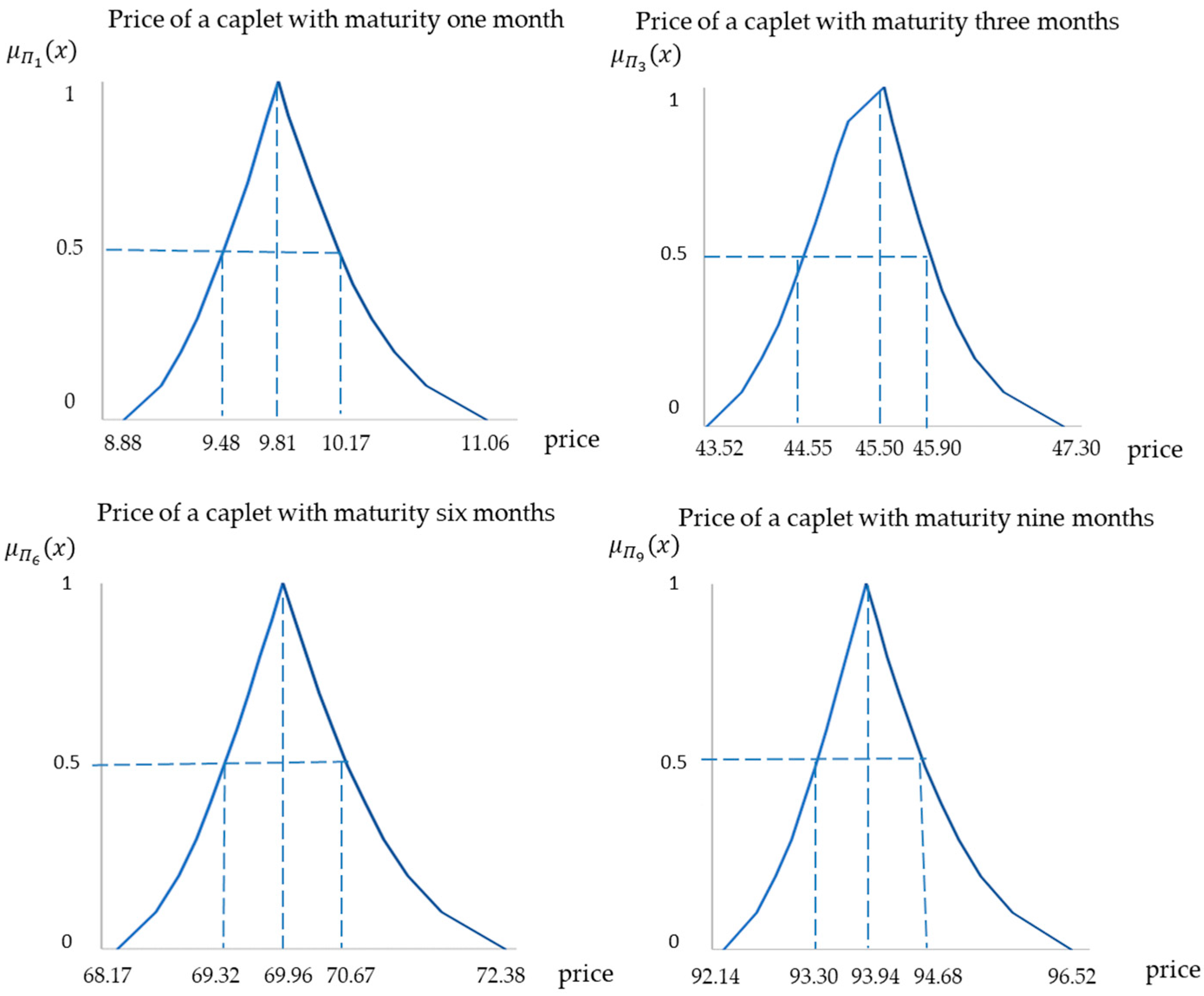
Empirical Application 1

The empirical application was developed for the European interbank bank on 17 March 2023. The rates were retrieved from https://www.euribor-rates.eu/en/, (accessed on 23 September 2024). In that market, spot rates and prices are provided for monthly maturities, as shown in Table 4 for the day we are analyzing. Thus, our binomial tree is constructed with monthly intervals, i.e., h = 1/12 years.
The point estimate of the volatility of short-term interest rates is derived from Equation (14) and considers the variation in the previous n = 60 sessions from 1 month to 17 March 2023. We obtain s d = 0.0003102 , which on an annual basis is s = 0.0003102 · 252 = 0.049243.
Similarly, for the α-cuts of fuzzy volatility ( σ α ), we must use (15)–(17). In these equations, we consider f γ , α = 1 2 γ 2 α + γ 2 , with γ = 0.05. Therefore, the volatilities used in this empirical application are as follows. From (15) and (16), we obtain the following:
σ d α = σ d 2 α = 59 · 0.0003102 2 χ 59 ; 0.475 α + 0.025 2 , 59 · 0.0003102 2 χ 59 ; 0.975 0.475 α 2 .
The core of σ d ~ is σ d 1 = 0.003102, and the support σ d 0 = [0.00026, 0.00038]. Likewise, from (17),
σ α = σ α _ , σ α ¯ = 252 · 59 · 0.0003102 2 χ 59 ; 0.475 α + 0.025 2 , 252 · 59 · 0.0003102 2 χ 59 ; 0.975 0.475 α 2 .
In this way, the core of σ ~ is σ 1 = 0 . 00495, and the rank of all possible values is σ 0 = [0.00418, 0.00600]. Figure 5 shows the shape of the annual volatility of one-month interest rates fitted with (15)–(17).
Figure 6 shows the fuzzy-binomial tree of one-month Euribor rates on 17 March, analogous to that shown in Figure 4, with the analytical fuzzy-random framework of Section 3.2, whose fuzzy version is implemented in Section 4.2. Thus, r i , 0 α , i = 1,2,…,11, is obtained from volatility (17) by applying (18). The remaining one-month rates in the ith period, r i , j α , j = 1,2,…, i , are obtained via (18) and (19).
Figure 7 displays the shape of the fuzzy number quantifying the price of a set of caplets over 1-month interest rates whose notional amount is 1,000,000 mu and K = 2.65%, with maturities of 1, 3, 6, and 9 months, which have been fitted from the yield rates shown in Figure 4. Whereas the cash flows in every scenario are fitted with (21), fitting the price requires the use of Equation (20). These estimates may allow a sensitivity analysis of the pricing model with respect to the expiration date of the caplet.
We have developed a naive comparison of our method by valuing four hypothetical caplets in the European interbank market, whose prices were calculated via our model in Figure 7, on a known online caplet calculator (https://quantcalc.net/BS76Caplet.html, accessed on 2 January 2025). For the caplet with a 1-month maturity, we obtained Π 1 = 9.96; for the 3-month maturity, Π 3 = 46.02; for the 6-month maturity, Π 3 = 69.88; for the 9-month maturity, Π 4 = 93.24. In all cases, the prices from the online calculator are included within the fuzzy estimate. Additionally, we can calculate the reliability degree of the value provided by the calculator according to our method, such that μ Π 1 ( 9.96 ) = 0.7, μ Π 3 ( 46.02 ) = 0.3, μ Π 6 ( 69.88 ) = 0.9, and μ Π 9 ( 93.24 ) = 0.4.
Thus, the fuzzy estimate provides a set of reasonable prices for the caplet that can serve as a reference for traders when setting the final price. This can be of particular interest in markets where caplets are typically traded, such as over-the-counter markets, where contracts are not standardized. Contracts in these markets are tailored to individual needs.

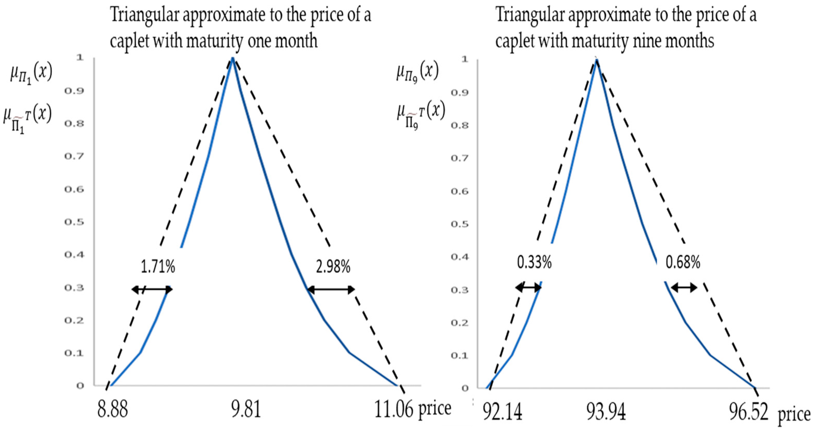
4.3. Adjusting a Triangular Fuzzy Number to Variables Linked to a Fuzzy Pricing of Interest-Sensitive Instruments with Ho and Lee’s Binomial Lattice

Although the α-cuts of the variables associated with the valuation of interest rate-sensitive instruments can provide accurate information on the shape of its membership function, an overly detailed description of interest and prices may complicate the overall interpretation of the results. Furthermore, the complex shapes of membership functions can produce drawbacks in calculations. Linear expressions are often sufficient to capture vagueness and provide manageable tools for processing and interpreting data [30].
Consequently, several approximation methods for FNs have been developed. Among these, triangular approximations have received significant attention, as they allow the resulting FN to be represented using only three parameters, namely, the lower and upper bounds of the support and the core, and they can be intuitively interpreted [73]. The aim of these approximations is to reduce computational effort and simplify interpretation simultaneously, achieving a balance between precision and practical use [73].
We evaluate the ability to approximate the variables embedded in our analysis (volatility, projected short-term interest rates, and derivative prices) using TFNs with the same support and core as the original FN. This simple approximation has been widely used in financial contexts, such as the final value of a pension plan [74], life insurance pricing [75], and option pricing [73]. Therefore, for an original FN a   ~ , its triangular approximation is denoted as a   ~ T = a ( 1 ) , a ( 2 ) , a ( 3 ) in such a way that from a 0 = a 0 _ , a 0 ¯ , a ( 1 ) = a 0 _ , and a ( 3 ) = a 0 ¯ from a 1 ,   a ( 2 ) = a 1 . Therefore, a α is approximated as
a α = a α _ , a α ¯ a α T _ , a α T ¯ = a ( 1 ) + a ( 2 ) a ( 1 ) α , a ( 3 ) a ( 3 ) a ( 2 ) α .
The accuracy of triangular approximations is measured by stating the relative errors in the extremes of the α-cuts of the original FN as follows:
e α _ = a α _ a α T _ a α _   a n d   e α ¯ = a α ¯ a α T ¯ a α ¯ .

Empirical Application 2

This empirical application is a continuation of empirical application 1. So, it was performed in the European interbank market on 17 March 2023. An analysis of the sensitivity of the goodness of fit of triangular approximations (22) with the measure of errors (23) is performed for annual volatility, as displayed in Figure 5; the lower and greater monthly yield rates in periods i = 1, 3, 6, 9, and 11 are embedded in Figure 6, and the fuzzy price of caplets is displayed in Figure 7. The detailed results of the sensitivity analysis, which were performed in α-cuts with eleven-point membership degrees α = 0, 0.1, …, 1, are shown in the annex. On the other hand, Figure 8, Figure 9 and Figure 10 display some of these results.
Table A1 in the annex and Figure 8 show that the triangular approximation (22) of volatility obtained empirically via (14)–(17) is quite accurate since the errors (23) in the sensitivity analysis are never greater than 3% (5%) in the lower (upper) extreme bounds of the α-level sets.
Figure 9 depicts the shapes of interest rates r 11,0 ~ ,   and r 11,11 ~ . Figure 6 shows their triangular approximations r 11,0 ~ T and r 11,11 ~ T obtained with (22). They suggest that their triangular approximation is accurate. Table A2 and Table A3 in the annex allow a more detailed analysis of the sensitivity analysis of the adequacy of the triangular approaches to monthly Euribor rates. These values are good enough since the errors in the extremes of the α-cuts are never greater than 3.5%. Moreover, we can intuit that these errors may increase with i and j, i.e., are greater in r ~ i + 1 , j than in r ~ i , j and in r ~ i , j + 1 than in r ~ i , j .
Figure 10 suggests that the price of caplets displayed in Figure 7 also has a reliable triangular approximate with the same support and core. Figure 10 and Table A4 in the annex show that the errors (23) of the caplet prices obtained with (20) and (21) in the sensitivity analysis are never greater than 3%, and they decrease with maturity. Therefore, these results allow us to intuit that our fuzzy methodology introduces uncertainty about the value of volatility by evaluating only three scenarios with conventional financial mathematics. Those linked with the greatest and smallest standard deviations come from the point estimate of short interest rate volatility. To do so and interpret the results does not require deep knowledge of fuzzy set theory but only financial knowledge of interest rate-sensitive instrument pricing.

5. Discussion

First, it offers a structured review of fuzzy-random option pricing in discrete time (FROPDT). Second, it expands upon fuzzy-random binomial lattices, which are widely used in FROPDT, to model yield rates and price instruments sensitive to interest rates. Binomial models are particularly popular in practical applications because of their combination of two valuable features: they are sufficiently flexible to model a variety of optionality types and provide a precise approximation of typical short-term interest rate stochastic processes used in continuous time [18].
We have checked that the scopes of the main outlets of the FROPDT are the wide fields of operational research and computational mathematics and, of course, the narrower soft computing and fuzzy mathematics settings. We have also observed contributions in financial and economic journals. The contributions to FROPDT steadily increased from the early 2000s to 2009. Since 2010, the literature has reached stationary production in such a way that FROPDT may be labeled a small but consolidated branch of fuzzy mathematics.
Mainstream FROPDT models use binomial lattices to represent price movements of the underlying asset and incorporate uncertainty in the up and down movements through fuzzy numbers (FNs), typically with a linear shape. As a result, risk-neutral probabilities also take the form of FNs. More intricate representations of uncertain parameters, such as intuitionistic fuzzy numbers, have rarely been applied in FROPDT, often within trinomial lattice frameworks.
Although the principal focus of fuzzy-binomial lattices has been on stock and index options and real options, conventional binomial lattices have been applied to a wide variety of financial pricing contexts, such as to fit the yield curve or to price the embedded options in mortgages [15]. However, the use of FROPDT in these fields is rare. In the field of interest-sensitive assets, we can outline only [27] who extends option games on bonds to fuzzy information of price and interest rate volatility.
This motivated the second contribution, which involves extending fuzzy-random binomial lattices to model the temporal structure of interest rates and to price interest rate options. Specifically, in a similar way to [27], it is grounded in Ho and Lee’s [11] binomial modeling of interest rates that, in continuous time, is equivalent to supposing normal fluctuations of short-term rates. Although this model, due to its simplicity, does not capture the full complexity of yield curve movements, it is widely used in the literature on the valuation of interest rate-sensitive instruments [6,20]. Therefore, we consider it worthwhile to study the algebraic aspects related to the implementation of this model with volatilities quantified using fuzzy numbers (FNs) and how these FNs can be derived from market data.
The findings of this paper indicate that the variables of binomial interest rate trees, such as volatility, future short-term rates, and option prices, are effectively approximated via triangular fuzzy numbers (TFNs). This suggests that implementing the proposed fuzzy-binomial approach with just three volatility scenarios (extremely high, extremely low, and most likely) can yield results comparable to those obtained by calculating numerous α-levels to achieve high computational accuracy.

6. Conclusions and Further Research

We believe that this work provides a comprehensive overview of FROPDT, which could be useful for researchers in applications of fuzzy mathematics to finance. This review highlights a clear research gap regarding the introduction of fuzzy uncertainty into fixed-income derivative valuation models in discrete time. This study has presented an application to the Ho and Lee model [11] with constant volatility, where the final adjustment using triangular fuzzy numbers is relatively straightforward.
One of the main criticisms of [11] is that it allows for negative short-term rates. However, this criticism does not apply to the environment in which we have developed the empirical application. During the 2010s, discount rates were persistently negative in several fixed-income markets, such as the European interbank market.
On the other hand, the Ho and Lee model [11] has other issues, such as its inability to account for variable volatilities or phenomena such as the volatility smile, which represents a weakness in the proposed model. Model [11] is a simplified model of interest rate dynamics. It may not accurately capture the complex behavior of real-world interest rates, especially during periods of significant market stress. This limitation could motivate future extensions to incorporate fuzziness in the parameters of binomial yield curve models, such as those of Black–Derman–Toy [12], Black–Karasinski [76], or Derman–Kani [77]. Furthermore, the implementation could consider the use of trinomial trees [45], which would require the use of fuzzy parameters. The use of trinomial trees in FROPDT has already been applied to options on stocks [67] and real options [44,46,50,65], making their application to fixed income a novel contribution.
The second objective of this study was to demonstrate that, from an analytical perspective, the forward induction [18] implemented with [11] when volatility is fuzzy is analytically feasible and, moreover, easily implementable and interpretable. Through intensive sensitivity analysis, we have verified that the model can be easily implemented using NBT, i.e., by considering expected volatility or with maximum reliability and two extreme volatilities, both high and low. We also showed that, on the analyzed day, the results provided by the proposed methodology align with those that could be offered by a broker. However, this result is far from definitive, as the model’s proximity to real-world practice would require a deep empirical analysis using market data from different time periods with heterogeneous volatility levels and interest rates. Empirical work in this regard, which also considers other alternatives such as trinomials or the use of discrete-time models adapted to fuzzy volatility [12,76,77], should be the subject of further research.
We have conducted empirical applications under the assumption that, apart from volatility, all the parameters are precise, a common approach in the fuzzy-binomial literature [34,35,36,38,39,48,52,53,56,59,63,66]. In this study, the options were priced using historical fuzzy volatility estimated through the method proposed by Sfiris and Papadopoulos [28]. Specifically, the volatility of short-term rates is derived by overlaying statistical confidence intervals on the variance of their daily fluctuations. Alternative approaches, such as fuzzy implicit volatility methods based on consistent probability-possibility transformations [78] or fuzzy regression techniques [79], present promising avenues for future research.
This study has extended the binomial yield curve model by assuming type-I fuzzy numbers. This approach restricts the information available to the decision-maker to a relatively simple representation. The use of more complex uncertainty models, such as type-II fuzzy numbers or intuitionistic fuzzy numbers, could address this drawback. Thus, a natural extension of FROPDT would be the use of such tools to model uncertainty in the parameters governing the stochastic movements of the prices of underlying assets in binomial lattices. However, introducing these tools may generate some challenges. Their use implies that calculations may become less parsimonious, input data may require the estimation of additional parameters, and analytical results may become harder to apply in practice.

Supplementary Materials

The following supporting information can be downloaded at: https://www.mdpi.com/article/10.3390/axioms14010052/s1: the PRISMA checklist.

Funding

This research received no external funding.

Data Availability Statement

Data used in this paper can be retrieved from https://www.euribor-rates.eu/en/ (accessed on 23 September 2024).

Acknowledgments

A preliminary draft of this paper has been published as a preprint in ResearchSquare (https://doi.org/10.21203/rs.3.rs-2777822/v1, accessed on 23 September 2024).

Conflicts of Interest

The author declares no conflict of interest.

Abbreviations

The following abbreviations are used in this manuscript:
FROPFuzzy-Random Option Pricing
FROPDTFuzzy-Random Option Pricing in Discrete Time
FNFuzzy Number
TFNTriangular Fuzzy Number
TrFNTrapezoidal Fuzzy Number

Appendix A

Table A1. A-cut representation for σ ~ d , σ ~ , and σ ~ d T , and sensitivity analysis of the errors of the triangular approximate.
α σ d _ α σ d ¯ α σ α _ σ α ¯ σ α T _ σ α T ¯ e α _ e α ¯
10.000310.000310.004950.004950.004950.004950.00%0.00%
0.90.000310.000320.004900.005010.004880.005060.48%0.99%
0.80.000310.000320.004850.005060.004800.005160.98%1.92%
0.70.000300.000320.004790.005120.004720.005271.47%2.78%
0.60.000300.000330.004740.005190.004640.005371.94%3.53%
0.50.000290.000330.004680.005260.004570.005472.37%4.15%
0.40.000290.000340.004610.005330.004490.005582.72%4.59%
0.30.000290.000340.004540.005420.004410.005682.93%4.76%
0.20.000280.000350.004460.005540.004330.005792.89%4.50%
0.10.000270.000360.004360.005700.004260.005892.31%3.43%
00.000260.000380.004180.006000.004180.006000.00%0.00%
Table A2. α-cuts of r i , 0 ~ for i = 1, 3, 6, 9, and 11, including their triangular approximations and the sensitivity analysis of the attained accuracy.
α-cuts of one-month interest rates r i , 0 ~
α r 1,0 α _ r 1,0 α ¯ r 3,0 α _ r 3,0 α ¯ r 6,0 α _ r 6,0 α ¯ r 9,0 α _ r 9,0 α ¯ r 11,0 α _ r 11,0 α ¯
10.025980.025980.027000.027000.025150.025150.023790.023790.022880.02288
0.90.025960.025990.026950.027050.025060.025250.023650.023930.022710.02305
0.80.025940.026010.026910.027090.024960.025340.023500.024070.022530.02322
0.70.025930.026020.026850.027140.024860.025430.023350.024210.022340.02339
0.60.025910.026040.026800.027190.024750.025530.023180.024350.022140.02357
0.50.025890.026060.026740.027240.024630.025630.023000.024510.021920.02376
0.40.025870.026070.026670.027290.024490.025740.022800.024670.021670.02395
0.30.025840.026090.026590.027350.024340.025860.022570.024850.021390.02418
0.20.025810.026120.026490.027430.024140.026000.022270.025060.021030.02444
0.10.025760.026150.026360.027520.023870.026180.021860.025330.020530.02477
00.025680.026200.026100.027670.023350.026490.021080.025800.019580.02533
α-cuts of one-month interest rates r i , 0 ~ r i , 0 ~ T = ( r i , 0 ( 1 ) , r i , 0 ( 2 ) r i , 0 ( 3 ) )
α r 1,0 T α _ r 1,0 T α ¯ r 3,0 T α _ r 3,0 T α ¯ r 6,0 T α _ r 6,0 T α ¯ r 9,0 T α _ r 9,0 T α ¯ r 11,0 T α _ r 11,0 T α ¯
10.025980.025980.027000.027000.025150.025150.023790.023790.022880.02288
0.90.025950.026000.026910.027070.024970.025290.023520.023990.022550.02313
0.80.025920.026020.026820.027140.024790.025420.023250.024190.022220.02337
0.70.025890.026040.026730.027200.024610.025550.022980.024390.021890.02362
0.60.025860.026070.026640.027270.024430.025690.022710.024590.021560.02386
0.50.025830.026090.026550.027340.024250.025820.022440.024790.021230.02411
0.40.025800.026110.026460.027400.024070.025960.022170.024990.020900.02435
0.30.025770.026130.026370.027470.023890.026090.021900.025190.020570.02460
0.20.025740.026150.026280.027540.023710.026220.021630.025400.020240.02484
0.10.025710.026180.026190.027600.023530.026360.021350.025600.019910.02509
00.025680.026200.026100.027670.023350.026490.021080.025800.019580.02533
Error (%)
e α _ e α ¯ e α _ e α ¯ e α _ e α ¯ e α _ e α ¯ e α _ e α ¯
10.00%0.00%0.00%0.00%0.00%0.00%0.00%0.00%0.00%0.00%
0.90.06%0.03%0.16%0.08%0.34%0.16%0.55%0.25%0.70%0.32%
0.80.11%0.05%0.31%0.15%0.68%0.32%1.09%0.51%1.39%0.64%
0.70.16%0.08%0.46%0.22%1.00%0.48%1.61%0.75%2.06%0.95%
0.60.20%0.10%0.60%0.29%1.30%0.62%2.09%0.97%2.70%1.22%
0.50.24%0.12%0.71%0.35%1.56%0.74%2.52%1.16%3.26%1.46%
0.40.27%0.14%0.80%0.40%1.76%0.84%2.86%1.30%3.71%1.64%
0.30.29%0.15%0.85%0.42%1.87%0.88%3.06%1.37%3.98%1.72%
0.20.28%0.14%0.82%0.40%1.82%0.85%2.99%1.32%3.90%1.64%
0.10.22%0.11%0.65%0.32%1.44%0.66%2.37%1.02%3.11%1.27%
00.00%0.00%0.00%0.00%0.00%0.00%0.00%0.00%0.00%0.00%
Table A3. α-cuts of r i , i ~ for i = 1, 3, 6, 9, and 11, including their triangular approximations and the sensitivity analysis of the attained accuracy.
α-cuts of one-month interest rates r i , i ~
α r 1,1 α _ r 1,1 α ¯ r 3,3 α _ r 3,3 α ¯ r 6,6 α _ r 6,6 α ¯ r 9,9 α _ r 9,9 α ¯ r 11,11 α _ r 11,11 α ¯
10.028840.028840.035580.035580.042310.042310.049520.049520.054340.05434
0.90.028790.028880.035440.035720.042030.042590.049100.049950.053820.05485
0.80.028740.028930.035300.035870.041750.042880.048680.050380.053300.05538
0.70.028690.028980.035150.036010.041460.043180.048240.050830.052770.05593
0.60.028640.029030.035000.036170.041150.043500.047790.051300.052220.05651
0.50.028590.029090.034840.036340.040830.043840.047310.051810.051620.05713
0.40.028530.029150.034660.036530.040480.044210.046780.052380.050980.05783
0.30.028460.029230.034460.036750.040080.044650.046180.053040.050250.05863
0.20.028380.029310.034230.037020.039600.045180.045460.053840.049370.05961
0.10.028280.029440.033910.037380.038960.045910.044500.054930.048200.06094
00.028090.029660.033340.038060.037830.047260.042800.056950.046120.06341
α-cuts of one-month interest rates r i , i ~ r i , i ~ T = ( r i , i ( 1 ) , r i , i ( 2 ) r i , i ( 3 ) )
α r 1,1 T α _ r 1,1 T α ¯ r 3,3 T α _ r 3,3 T α ¯ r 6,6 T α _ r 6,6 T α ¯ r 9,9 T α _ r 9,9 T α ¯ r 11,11 T α _ r 11,11 T α ¯
10.028840.028840.035580.035580.042310.042310.049520.049520.054340.05434
0.90.028760.028920.035360.035830.041860.042800.048850.050270.053510.05524
0.80.028690.029000.035130.036070.041410.043300.048180.051010.052690.05615
0.70.028610.029080.034910.036320.040960.043790.047510.051750.051870.05706
0.60.028540.029170.034680.036570.040520.044290.046840.052490.051050.05797
0.50.028460.029250.034460.036820.040070.044780.046160.053240.050230.05887
0.40.028390.029330.034230.037070.039620.045280.045490.053980.049410.05978
0.30.028310.029410.034010.037310.039170.045780.044820.054720.048580.06069
0.20.028240.029500.033790.037560.038720.046270.044150.055470.047760.06160
0.10.028160.029580.033560.037810.038280.046770.043470.056210.046940.06250
00.028090.029660.033340.038060.037830.047260.042800.056950.046120.06341
Error (%)
α e α _ e α ¯ e α _ e α ¯ e α _ e α ¯ e α _ e α ¯ e α _ e α ¯
10%0%0%0%0%0%0%0%0%0%
0.90.10%0.12%0.24%0.30%0.40%0.50%0.51%0.63%0.57%0.71%
0.80.19%0.24%0.47%0.58%0.80%0.97%1.03%1.23%1.16%1.37%
0.70.29%0.35%0.70%0.85%1.20%1.40%1.55%1.78%1.73%1.98%
0.60.37%0.45%0.92%1.09%1.57%1.79%2.04%2.27%2.28%2.51%
0.50.45%0.54%1.11%1.29%1.90%2.12%2.48%2.67%2.78%2.95%
0.40.50%0.61%1.25%1.44%2.17%2.35%2.83%2.96%3.19%3.27%
0.30.53%0.64%1.34%1.51%2.32%2.46%3.04%3.08%3.42%3.40%
0.20.52%0.61%1.30%1.45%2.26%2.35%2.98%2.94%3.37%3.23%
0.10.41%0.48%1.02%1.13%1.79%1.82%2.37%2.27%2.68%2.50%
00%0%0%0%0%0%0%0%0%0%
Table A4. Triangular approximates to the price of caplets in Figure 7 and sensitivity analysis of their accuracy.
1 Month3 Months6 Months9 Months
Π ~ i T =(8.88, 9.81, 11.06)(43.52, 45.40, 47.30)(68.17, 69.96, 72.38)(92.14, 93.94, 96.52)
α e α _ e α ¯ e α _ e α ¯ e α _ e α ¯ e α _ e α ¯
10.00%0.00%0.00%0.00%0.00%0.00%0.00%0.00%
0.90.29%0.60%0.43%0.22%0.08%0.16%0.06%0.14%
0.80.59%1.17%0.26%0.43%0.16%0.32%0.12%0.27%
0.70.88%1.70%0.10%0.64%0.24%0.47%0.18%0.39%
0.61.15%2.18%0.06%0.82%0.31%0.60%0.23%0.49%
0.51.40%2.57%0.21%0.99%0.37%0.72%0.28%0.58%
0.41.60%2.85%0.34%1.12%0.42%0.80%0.31%0.65%
0.31.71%2.98%0.44%1.21%0.45%0.84%0.33%0.68%
0.21.67%2.84%0.48%1.21%0.43%0.81%0.32%0.65%
0.11.32%2.19%0.41%0.93%0.34%0.63%0.25%0.51%
00.00%0.00%0.00%0.00%0.00%0.00%0.00%0.00%

References

  1. Zimmermann, H.; Hafner, W. Amazing discovery: Vincenz Bronzin’s option pricing models. J. Bank. Financ. 2007, 31, 531–546. [Google Scholar] [CrossRef]
  2. Constantinides, G.M. Black–Merton–Scholes Option Pricing: A 50-Year Celebration—Looking Ahead. J. Invest. Manag. 2024, 22, 11–15. [Google Scholar]
  3. Black, F.; Scholes, M. The pricing of options and corporate liabilities. J. Political Econ. 1973, 81, 637–654. Available online: http://www.jstor.org/stable/1831029 (accessed on 12 September 2024). [CrossRef]
  4. Merton, R.C. Theory of rational option pricing. Bell J. Econ. Manag. Sci. 1973, 4, 141–183. [Google Scholar] [CrossRef]
  5. Merton, R.C. Applications of option-pricing theory: Twenty-five years later. Am. Econ. Rev. 1998, 88, 323–349. Available online: http://www.jstor.org/stable/116838 (accessed on 12 September 2024).
  6. Chen, R.R. Understanding and Managing Interest Rate Risks; World Scientific: Singapore, 1996; Volume 1. [Google Scholar]
  7. Vasicek, O. An equilibrium characterization of the term structure. J. Financ. Econ. 1977, 5, 177–188. [Google Scholar] [CrossRef]
  8. Brennan, M.J.; Schwartz, E.S. A continuous time approach to the pricing of bonds. J. Bank. Financ. 1979, 3, 133–155. [Google Scholar] [CrossRef]
  9. Dothan, L.U. On the term structure of interest rates. J. Financ. Econ. 1978, 6, 59–69. [Google Scholar] [CrossRef]
  10. Cox, J.C.; Ingersoll, J.E., Jr.; Ross, S.A. An intertemporal general equilibrium model of asset prices. Econom. J. Econom. Soc. 1985, 53, 363–384. [Google Scholar] [CrossRef]
  11. Ho, T.S.; Lee, S.B. Term structure movements and pricing interest rate contingent claims. J. Financ. 1986, 41, 1011–1029. [Google Scholar] [CrossRef]
  12. Black, F.; Derman, E.; Toy, W. A one-factor model of interest rates and its application to treasury bond options. Financ. Anal. J. 1990, 46, 33–39. [Google Scholar] [CrossRef]
  13. Hull, J.; White, A. One-factor interest-rate models and the valuation of interest-rate derivative securities. J. Financ. Quant. Anal. 1993, 28, 235–254. [Google Scholar] [CrossRef]
  14. Hull, J.C. Options Futures and other Derivatives; Pearson Education India: Tamil Nadu, India, 2008. [Google Scholar]
  15. Trigeorgis, L. A log-transformed binomial numerical analysis method for valuing complex multioption investments. J. Financ. Quant. Anal. 1991, 26, 309–326. [Google Scholar] [CrossRef]
  16. Cox, J.; Ross, S.; Rubinstein, M. Option Pricing: A Simplified Approach. J. Financ. Econ. 1979, 7, 229–263. [Google Scholar] [CrossRef]
  17. Rendleman, R.J., Jr.; Bartter, B.J. Two state option pricing. J. Financ. 1979, 34, 1092–1110. [Google Scholar] [CrossRef]
  18. Jamshidian, F. Forward induction and construction of yield curve diffusion models. J. Fixed Income 1991, 1, 62–74. [Google Scholar] [CrossRef]
  19. Veronesi, P. Fixed Income Securities: Valuation, Risk, and Risk Management; Wiley: Hoboken, NJ, USA, 2010. [Google Scholar]
  20. Muzzioli, S.; De Baets, B. Fuzzy approaches to option price modeling. IEEE Trans. Fuzzy Syst. 2017, 25, 392–401. [Google Scholar] [CrossRef]
  21. Andrés-Sánchez, J. A systematic review of the interactions of fuzzy set theory and option pricing. Expert Syst. Appl. 2023, 223, 119868. [Google Scholar] [CrossRef]
  22. Cherubini, U.; Della Lunga, G. Fuzzy value-at-risk: Accounting for market liquidity. Econ. Notes 2001, 30, 293–312. [Google Scholar] [CrossRef]
  23. Collan, M.; Fuller, R.; Mezei, R. A Fuzzy Pay-Off Method for Real Option Valuation. J. Appl. Math. Decis. Sci. 2009, 2009, 238196. [Google Scholar] [CrossRef]
  24. Andrés-Sánchez, J. Fuzzy Random Option Pricing in Continuous Time: A Systematic Review and an Extension of Vasicek’s Equilibrium Model of the Term Structure. Mathematics 2023, 11, 2455. [Google Scholar] [CrossRef]
  25. Andrés-Sánchez, J. A Fuzzy-Random Extension of Jamshidian’s Bond Option Pricing Model and Compatible One-Factor Term Structure Models. Axioms 2023, 12, 668. [Google Scholar] [CrossRef]
  26. Jamshidian, F. An exact bond option formula. J. Financ. 1989, 44, 205–209. [Google Scholar] [CrossRef]
  27. Zmeškal, Z.; Dluhošová, D.; Gurný, P.; Guo, H. Soft bond game options valuation in discrete time using a fuzzy-stochastic approach. Int. J. Fuzzy Syst. 2022, 24, 2215–2228. [Google Scholar] [CrossRef]
  28. Sfiris, D.S.; Papadopoulos, B.K. Nonasymptotic fuzzy estimators based on confidence intervals. Inf. Sci. 2014, 279, 446–459. [Google Scholar] [CrossRef]
  29. Dubois, D.; Folloy, L.; Mauris, G.; Prade, H. Probability–possibility transformations, triangular fuzzy sets, and probabilistic inequalities. Reliab. Comput. 2004, 10, 273–297. [Google Scholar] [CrossRef]
  30. Kreinovich, V.O.; Kosheleva, S.N.; Shahbazova, S.N. Why triangular and trapezoid membership functions: A simple explanation. In Fuzziness and Soft Computing; Shahbazova, S., Sugeno, M., Eds.; Springer: Cham, Switzerland, 2020; Volume 391, pp. 25–31. [Google Scholar]
  31. Page, M.J.; McKenzie, J.E.; Bossuyt, P.M.; Boutron, I.; Hoffmann, T.C.; Mulrow, C.D.; Moher, D. The PRISMA 2020 statement: An updated guideline for reporting systematic reviews. BMJ 2021, 372, 71. [Google Scholar] [CrossRef]
  32. Zupic, I.; Čater, T. Bibliometric methods in management and organization. Organ. Res. Methods 2015, 18, 429–472. [Google Scholar] [CrossRef]
  33. Meyer, D.E.; Mehlman, D.W.; Reeves, E.S.; Origoni, R.B.; Evans, D.; Sellers, D.W. Comparison study of overlap among 21 scientific databases in searching pesticide information. Online Rev. 1983, 7, 33–43. [Google Scholar] [CrossRef]
  34. Yoshida, Y. A discrete-time model of American put option in an uncertain environment. Eur. J. Oper. Res. 2003, 151, 153–166. [Google Scholar] [CrossRef]
  35. Muzzioli, S.; Torricelli, C. A multiperiod binomial model for pricing options in a vague world. J. Econ. Dyn. Control 2004, 28, 861–887. [Google Scholar] [CrossRef]
  36. Lee, C.F.; Tzeng, G.-H.; Wang, S.-Y. A fuzzy set approach for generalized CRR model: An empirical analysis of S&P 500 index options. Rev. Quant. Financ. Account. 2005, 25, 255–275. [Google Scholar] [CrossRef]
  37. Buckley, J.J.; Eslami, E. Pricing stock options using fuzzy sets. Iran. J. Fuzzy Syst. 2015, 266, 131–143. [Google Scholar]
  38. Muzzioli, S.; Reynaerts, H. Option Pricing in the Presence of Uncertainty. In Perception-based Data Mining and Decision Making in Economics and Finance; Batyrshin, I., Kacprzyk, J., Sheremetov, L., Zadeh, L.A., Eds.; Studies in Computational Intelligence; Springer: Berlin/Heidelberg, Germany, 2007; Volume 36. [Google Scholar] [CrossRef]
  39. Buckley, J.J.; Eslami, E. Pricing Options, Forwards and Futures Using Fuzzy Set Theory. Fuzzy Eng. Econ. Appl. 2008, 233, 339–357. [Google Scholar] [CrossRef]
  40. Muzzioli, S.; Reynaerts, H. American option pricing with imprecise risk-neutral probabilities. Int. J. Approx. Reason. 2008, 44, 1303–1321. [Google Scholar] [CrossRef]
  41. Liao, S.H.; Ho, S.H. Investment project valuation based on a fuzzy binomial approach. Inf. Sci. 2010, 180, 2124–2133. [Google Scholar] [CrossRef]
  42. Wang, B.; Wang, S.; Watada, J. Real options analysis based on fuzzy random variables. Int. J. Innov. Comput. Inf. Control 2010, 6, 1689–1698. [Google Scholar]
  43. Zmeskal, Z. Generalized soft binomial American real option pricing model (fuzzy-stochastic approach). Eur. J. Oper. Res. 2010, 207, 1096–1103. [Google Scholar] [CrossRef]
  44. Tolga, A.Ç.; Kahraman, C.; Demircan, M.L. A Comparative Fuzzy Real Options Valuation Model using Trinomial Lattice and Black-Scholes Approaches: A Call Center Application. J. Mult. Valued Log. Soft Comput. 2010, 16, 135–154. [Google Scholar]
  45. Hull, J.; White, A. Numerical procedures for implementing term structure models I: Single-factor models. J. Deriv. 1994, 2, 7–16. [Google Scholar] [CrossRef]
  46. Allenotor, D.; Thulasiram, R.K. Grid resources valuation with fuzzy real option. Int. J. High Perform. Comput. Netw. 2011, 7, 1–7. [Google Scholar] [CrossRef]
  47. Ho, S.H.; Liao, S.H. A fuzzy real option approach for investment. Expert Syst. Appl. 2011, 38, 15296–15302. [Google Scholar] [CrossRef]
  48. Yu, S.-E.; Huarng, K.-H.; Leon Li, M.-Y.; Chen, C.-Y. A novel option pricing model via fuzzy binomial decision tree. Int. J. Innov. Comput. Inf. Control 2011, 7, 709–718. [Google Scholar]
  49. Elahi, Y.; Aziz MI, A. Efficient pricings for binomial Asian option under fuzzy environment. Far East J. Math. Sci. 2012, 63, 133–140. Available online: https://www.pphmj.com/abstract/6564.htm (accessed on 12 September 2024).
  50. Tolga, A.C.; Tuysuz, F.; Kahraman, C. A fuzzy multi-criteria decision analysis approach for retail location selection. Int. J. Inf. Technol. Decis. Mak. 2013, 12, 729–755. [Google Scholar] [CrossRef]
  51. Cruz Aranda, F.; Ortiz Arango, F.; Cabrera Llanos, A.I. Project valuation of a distribution centre of an auxiliary rail freight terminal: Using real options with fuzzy logic and binomial trees. J. Appl. Econ. Sci. 2016, 12, 894–905. Available online: https://www.ceeol.com/search/article-detail?id=534332 (accessed on 12 September 2024).
  52. Anzilli, L.; Facchinetti, G. New definitions of mean value and variance of fuzzy numbers: An application to the pricing of life insurance policies and real options. Int. J. Approx. Reason. 2017, 91, 96–113. [Google Scholar] [CrossRef]
  53. Anzilli, L.; Facchinetti, G.; Pirotti, T. Pricing of minimum guarantees in life insurance contracts with fuzzy volatility. Inf. Sci. 2018, 460, 578–593. [Google Scholar] [CrossRef]
  54. Xu, W.J.; Liu, G.F.; Yu, X.J. A Binomial Tree Approach to Pricing Vulnerable Option in a Vague World. Int. J. Uncertain. Fuzziness Knowl. Based Syst. 2018, 26, 143–162. [Google Scholar] [CrossRef]
  55. Zhang, H.; Watada, J. Fuzzy Levy-GJR-GARCH American option pricing model based on an infinite pure jump process. IEICE Trans. Inf. Syst. 2018, 101, 1843–1859. [Google Scholar] [CrossRef]
  56. D’Amato, M.; Zrobek, S.; Bilozor, M.R.; Walacik, M.; Mercadante, G. Valuing the effect of the change of zoning on underdeveloped land using fuzzy real option approach. Land Use Policy 2019, 86, 365–374. [Google Scholar] [CrossRef]
  57. Cruz Aranda, F.; Terán Bustamante, A. Valuation of an investment project in research and development in the pharmaceutical industry. Contaduría Y Adm. 2019, 64, 90. [Google Scholar] [CrossRef]
  58. Meenakshi, K.; Felbin, C. Problem of Pricing American Fuzzy Put Option Buyers Model for general Trapezoidal Fuzzy Numbers. Recent Trends Parallel Comput. 2016, 25, 402–416. [Google Scholar] [CrossRef]
  59. Shang, T.C.; Yang, L.; Liu, P.H.; Shang, K.T.; Zhang, Y. Financing mode of energy performance contracting projects with carbon emissions reduction potential and carbon emissions ratings. Energy Policy 2020, 144, 111632. [Google Scholar] [CrossRef]
  60. Chrysafis, K.A.; Papadopoulos, B.K. Decision Making for Project Appraisal in Uncertain Environments: A Fuzzy-Possibilistic Approach of the Expanded NPV Method. Symmetry 2021, 13, 27. [Google Scholar] [CrossRef]
  61. Meenakshi, K.; Kennedy, F.C. A study of european fuzzy put option buyers model on future contracts involving general trapezoidal fuzzy numbers. Glob. Stoch. Anal. 2021, 8, 47–59. [Google Scholar]
  62. Meenakshi, K.; Kennedy, F.C. On some properties of American fuzzy put option model on fuzzy future contracts involving general linear octagonal fuzzy numbers. Adv. Appl. Math. Sci. 2021, 21, 331–342. [Google Scholar]
  63. Wang, G.X.; Wang, Y.Y.; Tang, J.M. Fuzzy Option Pricing Based on Fuzzy Number Binary Tree Model. IEEE Trans. Fuzzy Syst. 2021, 30, 3548–3558. [Google Scholar] [CrossRef]
  64. Zmeskal, Z.; Dluhosova, D.; Gurny, P.; Kresta, A. Generalized soft multimode real options model (fuzzy-stochastic approach). Expert Syst. Appl. 2022, 192, 116388. [Google Scholar] [CrossRef]
  65. Ersen, H.Y.; Tas, O.; Ugurlu, U. Solar Energy Investment Valuation With Intuitionistic Fuzzy Trinomial Lattice Real Option Model. IEEE Trans. Eng. Manag. 2023, 70, 2584–2593. [Google Scholar] [CrossRef]
  66. Zhang, X.Y.; Yin, J.B. Assessment of investment decisions in bulk shipping through fuzzy real options analysis. Marit. Econ. Logist. 2023, 25, 122–139. [Google Scholar] [CrossRef]
  67. Agustina, F.; Sumarti, N.; Sidarto, K.A. Construction of the bino-trinomial method using the fuzzy set approach for option pricing. J. Indones. Math. Soc. 2024, 30, 179–204. [Google Scholar] [CrossRef]
  68. Kamrad, B.; Ritchken, P. Multinomial Approximating Models for Options with k State Variables. Manag. Sci. 1991, 37, 197–210. [Google Scholar] [CrossRef]
  69. Andrés-Sánchez, J.D. Modeling Up-and-Down Moves of Binomial Option Pricing with Intuitionistic Fuzzy Numbers. Axioms 2024, 13, 503. [Google Scholar] [CrossRef]
  70. Buckley, J.J. Fuzzy statistics: Hypothesis testing. Soft Comput. 2005, 9, 512–518. [Google Scholar] [CrossRef]
  71. Chrysafis, K.A.; Papadopoulos, B.K. On theoretical pricing of options with fuzzy estimators. J. Comput. Appl. Math. 2009, 223, 552–566. [Google Scholar] [CrossRef]
  72. Buckley, J.J.; Qu, Y. On using α-cuts to evaluate fuzzy equations. Fuzzy Sets Syst. 1990, 38, 309–312. [Google Scholar] [CrossRef]
  73. Andres-Sanchez, J. Pricing European Options with Triangular Fuzzy Parameters: Assessing Alternative Triangular Approximations in the Spanish Stock Option Market. Int. J. Fuzzy Syst. 2018, 20, 1624–1643. [Google Scholar] [CrossRef]
  74. Jiménez, M.; Rivas, J.A. Fuzzy number approximation. Int. J. Uncertain. Fuzziness Knowl. Based Syst. 1998, 6, 69–78. [Google Scholar] [CrossRef]
  75. Andrés-Sánchez, J.; Puchades, L.G.V. Life settlement pricing with fuzzy parameters. Appl. Soft Comput. 2023, 148, 110924. [Google Scholar] [CrossRef]
  76. Black, F.; Karasinski, P. Bond and Option pricing when Short rates are Lognormal. Financ. Anal. J. 1991, 47, 52–59. [Google Scholar] [CrossRef]
  77. Derman, E.; Kani, I. Riding on a smile. Risk 1994, 7, 32–39. [Google Scholar]
  78. Capotorti, A.; Figà-Talamanca, G. SMART-or and SMART-and fuzzy average operators: A generalized proposal. Fuzzy Sets Syst. 2020, 395, 1–20. [Google Scholar] [CrossRef]
  79. Muzzioli, S.; Ruggieri, A.; De Baets, B. A comparison of fuzzy regression methods for the estimation of the implied volatility smile function. Fuzzy Sets Syst. 2015, 266, 131–143. [Google Scholar] [CrossRef]
Figure 2. Temporal evolution of contributions to FROPDT from 2000.
Axioms 14 00052 g002
Figure 3. Number of contributions to fuzzy-random pricing in discrete time by country since 2000.
Axioms 14 00052 g003
Figure 4. Recombinant binomial lattices of short-term interest rates and Arrow–Debreu assets. Note: r i j represents the interest rate in the jth state of the ith period, and d i j represents the price of an Arrow–Debreu asset that matures in the ith period and is in the jth state.
Axioms 14 00052 g004
Figure 5. Fuzzy volatility of one-month interest rates in the European interbank market on 17 March 2023.
Axioms 14 00052 g005
Figure 6. Fuzzy-binomial tree of the interbank European market on 17 March 2023 and one-month rates during the next year. Note: values are presented as percentages.
Axioms 14 00052 g006
Figure 7. Shapes of the membership functions for the prices of caplets on monthly interest rates over a notional amount of 100,000 monetary units, K = 2.65%, and several maturities.
Axioms 14 00052 g007
Figure 8. Representation of σ ~ and σ ~ T , and the maximum errors of the triangular approximate. Note: The solid line represents the fitted volatility σ ~ , and the dashed line represents the triangular approximate σ ~ T .
Axioms 14 00052 g008
Figure 9. Representation of r 11,0 ~ ,   and r 11,11 ~ , their triangular approximations r 11,0 ~ T and r 11,11 ~ T , and maximum errors of the triangular approximate. Note: The solid line represents r 11,0 ~   and r 11,11 ~ , and the dashed line represents the triangular approximates r 11,0 ~ T and r 11,11 ~ T .
Axioms 14 00052 g009
Figure 10. Representation of the fuzzy prices of the caplets with maturities at 1 month and 9 months, their triangular approximations and the maximum errors. Note: The solid line represents the fuzzy price in Figure 7, and the dashed line represents the triangular approximation.
Axioms 14 00052 g010
Table 2. Journals with contributions to FROPDT.
JournalNumber of Items
Expert Systems with Applications3
European Journal of Operational Research
IEEE Transactions of Fuzzy Systems
Information Sciences
International Journal of Approximate Reasoning
Journal of Innovative Computing, Information and Control
2
Advances and Applications in Mathematical Sciences; Axioms; Contaduría y Administración; Energy Policy; Far East Journal of Mathematical Sciences; Fuzzy Engineering Economics with Applications (book); Global and Stochastic Analysis; IEICE Transactions on Information and Systems; IEEE Transactions on Engineering Management; International Journal of Fuzzy Systems; International Journal of High Performance Computing and Networking; International Journal of Information Technology & Decision Making; International Journal of Uncertainty Fuzziness and Knowledge-Based Systems; Iranian Journal of Fuzzy Systems; Journal of Economic Dynamics & Control; Journal of Applied Economic Sciences; Journal of Marine Science and Technology-Taiwan; Journal of the Indonesian Mathematical Society; Land Use Policy; Maritime Economics & Logistics; Perception-Based Data Mining and Decision Making in Economics and Finance; Recent Trends in Parallel Computing; Review of Quantitative Finance and Accounting; Symmetry-Basel1
Table 3. Papers with more than 10 citations in the SCOPUS or WoS databases.
AuthorsYearTitleJournalSCOPUSWoS
Muzzioli and Torricelli [35]2004A multiperiod binomial model for pricing options in a vague world.Journal of Economic Dynamics & Control6772
Zmeskal [43]2010Generalized soft binomial American real option pricing model (fuzzy-stochastic approach).European Journal of Operational Research5564
Ho and Liao [47]2011A fuzzy real option approach for investment.Expert Systems With Applications5556
Yoshida [34]2003A discrete-time model of American options in an uncertain environment. European Journal of Operational Research4340
Muzzioli and Reynaerts [39]2008American option pricing with imprecise risk-neutral probabilities.International Journal of Approximate Reasoning3934
Liao and Ho [41]2010Investment project valuation based on a fuzzy-binomial approach.Information Sciences3735
Muzzioli and de Baets [20]2017Fuzzy approaches to option price modeling.IEEE Transactions on Fuzzy Systems3838
Lee et al. [36]2005A fuzzy set approach for the generalized CRR model: an empirical analysis of S&P 500 index options.Review of Quantitative Finance and Accounting33NO
Yu et al. [48]2011Model construction of option pricing based on fuzzy theory.Journal of Marine Science and Technology-Taiwan1833
Shang et al. [59]2020Financing mode of energy performance contracting projects with carbon emissions reduction potential and carbon emissions ratings.Energy Policy2519
D’Amato et al. [56]2019Valuing the effect of the change in zoning on underdeveloped land using the fuzzy real options approach.Land Use Policy1912
Chrysafis and Papadopoulos [60]2021Decision making for project appraisal in uncertain environments: a fuzzy-possibilistic approach of the expanded NPV method.Symmetry1817
Andrés-Sánchez [69]2023aA systematic review of the interactions of fuzzy set theory and option pricing.Expert Systems with Applications1213
Table 4. Instantaneous spot rates in the interbank European market on 17 March 2023.
Month (maturity)1 month
(17 April 2023)
2 months
(17 May 2023)
3 months (17 June 2023)4 months (17 July 2023)5 months
(17 August 2023)
6 months
(17 September 2023)
spot rate2.6452.6932.7412.8382.9353.032
price99.78099.55299.31799.05998.78598.495
Month (maturity)7 months
(17 October 2023)
8 months
(17 November 2023)
9 months
(17 December 2023)
10 months
(17 January 2024)
11 months
(17 February 2023)
12 months
(17 March 2023)
spot rate3.0813.1293.1783.2273.2753.324
price98.21997.93597.64597.34797.04296.731
Disclaimer/Publisher’s Note: The statements, opinions and data contained in all publications are solely those of the individual author(s) and contributor(s) and not of MDPI and/or the editor(s). MDPI and/or the editor(s) disclaim responsibility for any injury to people or property resulting from any ideas, methods, instructions or products referred to in the content.

