Article

Threshold Dynamics of Honey Bee Colonies with General Eclosion and Social Inhibition

by
Md Mostafizur Rahaman
and
Xiang-Sheng Wang
*
Department of Mathematics, University of Louisiana at Lafayette, Lafayette, LA 70503, USA
*
Author to whom correspondence should be addressed.
Axioms 2025, 14(10), 773; https://doi.org/10.3390/axioms14100773
Submission received: 11 August 2025 / Revised: 23 September 2025 / Accepted: 20 October 2025 / Published: 21 October 2025
(This article belongs to the Special Issue Trends in Dynamical Systems and Applied Mathematics)

Abstract

Honey bee colonies are important to worldwide agriculture and the health of natural ecosystems. Understanding the factors behind colony persistence and failure has been a major challenge for both ecologists and mathematicians. In this paper, we present a general mathematical model to explore the threshold dynamics of honey bee colonies. We explicitly define the basic reproduction number in terms of model parameters and demonstrate its critical role in determining whether a colony survives or collapses. We offer a biological interpretation of the basic reproduction number and prove the threshold dynamics for the general model system. Our results are established using dynamical systems techniques, including the comparison principle, persistence theory, linearization, and global analysis. For specifically chosen eclosion and social inhibition functions, we perform a sensitivity analysis to determine how the basic reproduction number depends on the model parameters.

1. Introduction

Honey bees (Apis mellifera) play a vital role in global agriculture and natural ecosystems by providing essential pollination services [1]. However, honey bee populations in North America and the United Kingdom have been in decline since the 1940s [2,3,4]. According to the USDA National Agricultural Statistics Service [5], there were 4.3 million honey-producing colonies in 1976 and 3.3 million in 1989. In contrast, the figures for the most recent five years (2020–2024) were 2.71, 2.70, 2.67, 2.51, and 2.60 million, respectively. Over the past two decades, researchers have investigated the causes underlying honey bee colony failures [6]. In [7], the authors develop a mathematical model to investigate how variations in food availability interact with forager mortality to affect colony growth. The population dynamics of honey bee colonies are examined in [8] using both smooth and non-smooth modeling approaches.
The complexity and nonlinearities of the aforementioned models pose significant challenges for the mathematical analysis of honey bee dynamics. Therefore, it is essential to employ dynamical systems theory to examine the effects of key factors on the persistence or collapse of honey bee colonies. The aim of this study is to establish a mathematical framework for investigating the population dynamics of honey bee colonies. A crucial step in this framework is the definition of a biologically meaningful threshold parameter, the basic reproduction number. In ecological systems, the value of this parameter determines whether a population persists or becomes extinct, whereas in epidemiological models, it serves as a key indicator of whether a disease will persist or disappear.
In this study, we use a general mathematical model to analyze the threshold dynamics that govern honey bee colony survival. In particular, we derive a critical threshold parameter that determines whether a colony will collapse or persist over time. The worker population of the honey bee is divided into two groups: hive bees, which carry out various tasks inside the nest, such as raising brood, and forager bees, which specialize in collecting food and materials [9]. Hence, we propose the following two-compartmental model of honey bee colonies:
H ( t ) = b ( H ( t ) , F ( t ) ) ( d + α ) H ( t ) + r ( H ( t ) , F ( t ) ) ,
F ( t ) = α H ( t ) m F ( t ) r ( H ( t ) , F ( t ) ) ,
where H ( t ) and F ( t ) , respectively, denote the populations of hive bees and forager bees at time t. The eclosion rate is given by a general nonlinear function b ( H , F ) . The death rates of the hive bees and forager bees are d and m, respectively. The transition rate from hive bees to forager bees is α . The social inhibition is modeled by the nonlinear function r ( H , F ) . The hive-to-forager transition and social inhibition enhance colony growth, development, and environmental adaptation [10].
We adopt the following notations throughout this paper. We use R + = [ 0 , ) to denote the set of non-negative real numbers. For any positive integer n, the set of non-negative vectors is denoted by R + n . We say a vector v R + n is positive if each element of v is positive. If g C 1 ( R + 2 , R ) is a differential function with two variables x and y, then we denote the partial derivative functions as follows:
g 1 = x g , g 2 = y g .
If g C 2 ( R + 2 , R ) is second-order differentiable, then we denote the second-order partial derivative functions as follows:
g 11 = x x 2 g , g 12 = x y 2 g , g 21 = y x 2 g , g 22 = y y 2 g .
Clearly, we have g 12 = g 21 . For a square matrix M R n × n , the spectral radius and the determinant of M are denoted as ρ ( M ) and det ( M ) , respectively. Let λ 1 , , λ n be the eigenvalues (counting multiplicity) of M, we have the following:
ρ ( M ) = max 1 j n | λ j | , det ( M ) = j = 1 n λ j .
We shall make some basic biological assumptions on our model system. First, the constants d, m and α are positive. Next, the initial values H ( 0 ) and F ( 0 ) are non-negative with H ( 0 ) + F ( 0 ) > 0 . Finally, we assume that the functions b ( x , y ) and r ( x , y ) satisfy the following conditions:
(C1)
b C 2 ( R + 2 , R + ) with b ( 0 , 0 ) = 0 , b ( x , y ) L , b 1 ( x , y ) 0 and b 2 ( x , y ) 0 for ( x , y ) R + 2 .
(C2)
r C 2 ( R + 2 , R + ) with r ( x , 0 ) = 0 , r 1 ( x , y ) 0 and r 2 ( x , y ) 0 for ( x , y ) R + 2 .
The biological interpretations of conditions (C1)–(C2) are as follows. No eclosion occurs if both hive bees and forager bees are absent. The eclosion rate increases with the populations of hive bees and forager bees; however, it is bounded above by a maximal rate L. The social inhibition rate rises with the population of forager bees and decreases with the population of hive bees, and no social inhibition occurs in the absence of forager bees.

2. Results

2.1. Positiveness and Ultimate Boundedness

Proposition 1.
Assume (C1)–(C2). The system (1) and (2) with positive initial values possesses a global unique solution ( H ( t ) , F ( t ) ) R + 2 that is positive for all t 0 . Moreover, we have the following:
lim sup t [ H ( t ) + F ( t ) ] L min { d , m } ;
that is, the solution is ultimately bounded by a constant independent of the initial values.
Proof. 
Given any positive initial values H ( 0 ) > 0 and F ( 0 ) > 0 , we apply the standard theory of ordinary differential equations to obtain that the solution exists on a maximal interval [ 0 , T ) , where either T = or | H ( t ) | + | F ( t ) | as t T .
First, we claim that H ( t ) > 0 and F ( t ) > 0 for all t [ 0 , T ) . If not, then there exists t 1 ( 0 , T ) such that H ( t ) F ( t ) 0 for t [ 0 , t 1 ) and H ( t 1 ) F ( t 1 ) = 0 . By continuity of the solution, we have H ( t ) > 0 and F ( t ) > 0 for all t [ 0 , t 1 ) . Hence, the conditions (C1)–(C2) imply that b ( H ( t ) , F ( t ) ) + r ( H ( t ) , F ( t ) ) 0 for all t [ 0 , t 1 ) . Now, we obtain the following from (1):
0 0 t 1 e ( d + α ) t [ b ( H ( t ) , F ( t ) ) + r ( H ( t ) , F ( t ) ) ] d t = 0 t 1 e ( d + α ) t [ H ( t ) + ( d + α ) H ( t ) ] d t = e ( d + α ) t 1 H ( t 1 ) H ( 0 ) .
Since H ( 0 ) > 0 , we have H ( t 1 ) > 0 . From the choice of t 1 we obtain F ( t 1 ) = 0 . It then follows from (2) and (C2) that F ( t 1 ) = α H ( t 1 ) > 0 . Recall that F ( t ) > 0 for t [ 0 , t 1 ) . We obtain F ( t 1 ) > 0 , which is a contradiction. Hence, we have proved that the solution remains positive for all t [ 0 , T ) .
Next, we add the two Equations (1) and (2) and make use of (C1) to find the following:
H ( t ) + F ( t ) = b ( H ( t ) , F ( t ) ) d H ( t ) m F ( t ) L μ [ H ( t ) + F ( t ) ] ,
where μ : = min { m , d } > 0 . In particular, H ( t ) + F ( t ) H ( 0 ) + F ( 0 ) + L t for all t [ 0 , T ) , which implies that the solution cannot blow up at finite time. Hence, T = . Moreover, the above differential inequality implies that
lim sup t [ H ( t ) + F ( t ) ] L μ .
This completes the proof. □

2.2. Basic Reproduction Number

On account of (C1)–(C2), our model system (1) and (2) possesses a trivial equilibrium E 0 = ( 0 , 0 ) . We linearize the system about this trivial equilibrium and obtain the following:
H ( t ) F ( t ) = A H ( t ) F ( t ) , A = b 1 ( 0 , 0 ) ( d + α ) + r 1 ( 0 , 0 ) b 2 ( 0 , 0 ) + r 2 ( 0 , 0 ) α r 1 ( 0 , 0 ) m r 2 ( 0 , 0 ) .
We split A = B V , where the following is then calculated:
B = b 1 ( 0 , 0 ) b 2 ( 0 , 0 ) 0 0 , V = d + α r 1 ( 0 , 0 ) r 2 ( 0 , 0 ) α + r 1 ( 0 , 0 ) m + r 2 ( 0 , 0 ) .
In view of (C1)–(C2), this is a regular splitting [11] in the sense that B is a non-negative matrix and V is a nonsingular matrix with a non-negative inverse, written as follows:
V 1 = 1 det ( V ) m + r 2 ( 0 , 0 ) r 2 ( 0 , 0 ) α r 1 ( 0 , 0 ) d + α r 1 ( 0 , 0 ) ,
where
det ( V ) = [ d + α r 1 ( 0 , 0 ) ] [ m + r 2 ( 0 , 0 ) ] r 2 ( 0 , 0 ) [ α r 1 ( 0 , 0 ) ] = d [ m + r 2 ( 0 , 0 ) ] + m [ α r 1 ( 0 , 0 ) ] > 0 .
The basic reproduction number [12,13] is defined as the spectral radius of the next generation matrix B V 1 , written as follows:
R 0 = ρ ( B V 1 ) = b 1 ( 0 , 0 ) [ m + r 2 ( 0 , 0 ) ] + b 2 ( 0 , 0 ) [ α r 1 ( 0 , 0 ) ] d [ m + r 2 ( 0 , 0 ) ] + m [ α r 1 ( 0 , 0 ) ] .
To interpret the biological meaning of the basic reproduction number, we shall define the effective transition rate from hive bees to forager bees as follows:
H 2 F = [ α r 1 ( 0 , 0 ) ] · m m + r 2 ( 0 , 0 ) .
Recall that d is the death rate of the hive bees. The average life span of hive bees is calculated as follows:
L S H = 1 d + H 2 F .
For each hive bee, during its lifespan, the average number of new hive bees produced in the next generation is calculated as follows:
L S H · b 1 ( 0 , 0 ) + L S H · H 2 F · L S F · b 2 ( 0 , 0 ) ,
where L S F = 1 / m is the average lifespan of forager bees. A simple calculation shows that the above quantity is the same as R 0 defined in (5).

2.3. Stability of Trivial Equilibrium

Theorem 1.
Assume (C1)–(C2). Let R 0 be defined as in (5). The trivial equilibrium E 0 = ( 0 , 0 ) of system (1) and (2) is locally asymptotically stable if R 0 < 1 and unstable if R 0 > 1 .
Proof. 
The determinant of A in (3) can be calculated as follows:
det ( A ) = [ d + α r 1 ( 0 , 0 ) b 1 ( 0 , 0 ) ] [ m + r 2 ( 0 , 0 ) ] [ α r 1 ( 0 , 0 ) ] [ b 2 ( 0 , 0 ) + r 2 ( 0 , 0 ) ] = [ d b 1 ( 0 , 0 ) ] [ m + r 2 ( 0 , 0 ) ] + [ m b 2 ( 0 , 0 ) ] [ α r 1 ( 0 , 0 ) ] .
If R 0 < 1 , then det ( A ) > 0 . Moreover, since m + r 2 ( 0 , 0 ) > 0 , α r 1 ( 0 , 0 ) > 0 , and b 2 ( 0 , 0 ) + r 2 ( 0 , 0 ) 0 , we have d + α r 1 ( 0 , 0 ) b 1 ( 0 , 0 ) > 0 , and hence the trace of A is negative. Therefore, both eigenvalues of A have negative real parts. This implies local asymptotic stability of E 0 .
On the other hand, if R 0 > 1 , then det ( A ) < 0 and A possesses a positive eigenvalue. Thus, the trivial equilibrium E 0 is unstable. □
Theorem 2.
Assume (C1)–(C2). Let R 0 be defined as in (5). If R 0 = 1 , then the trivial equilibrium E 0 = ( 0 , 0 ) of system (1) and (2) is locally asymptotically stable if η < 0 and unstable if η > 0 , where the following is calculated:
η = j = 1 2 k = 1 2 { [ m + r 2 ( 0 , 0 ) ] b j k ( 0 , 0 ) + [ m b 2 ( 0 , 0 ) ] r j k ( 0 , 0 ) } w j w k
with w 1 = m + r 2 ( 0 , 0 ) and w 2 = α r 1 ( 0 , 0 ) .
Proof. 
Since R 0 = 1 , we have det ( A ) = 0 . Moreover, 0 is a simple eigenvalue of A with a positive left eigenvector, written as follows:
v = m + r 2 ( 0 , 0 ) b 2 ( 0 , 0 ) + r 2 ( 0 , 0 )
and a positive right eigenvector
w = m + r 2 ( 0 , 0 ) α r 1 ( 0 , 0 ) .
We denote the following:
η = j = 1 2 k = 1 2 { [ m + r 2 ( 0 , 0 ) ] [ b j k ( 0 , 0 ) + r j k ( 0 , 0 ) ] [ b 2 ( 0 , 0 ) + r 2 ( 0 , 0 ) ] r j k ( 0 , 0 ) } w j w k .
By Theorem 1 in [14], we obtain that E 0 is locally asymptotically stable if η < 0 and unstable if η > 0 . It is easily seen that η can be simplified as in (6). This completes the proof. □

2.4. Uniform Persistence

We first state a lemma that will be used frequently.
Lemma 1.
Consider a matrix written as follows:
M = M 11 M 12 M 21 M 22 R 2 × 2 .
(a) 
If det ( M ) < 0 , M 12 > 0 and M 22 < 0 , then M has a positive eigenvalue λ > 0 with a positive left eigenvector ( c 1 , c 2 ) , where c 1 = λ M 22 > 0 and c 2 = M 12 > 0 .
(b) 
If det ( M ) < 0 , M 12 < 0 and M 22 < 0 , then M has a positive eigenvalue λ > 0 with a left eigenvector ( c 1 , c 2 ) , where c 1 = λ M 22 > 0 and c 2 = M 12 > 0 .
(c) 
If det ( M ) 0 , M 12 > 0 , M 21 > 0 , and M 22 < 0 , then M 11 < 0 and M has two simple eigenvalues λ 1 and λ 2 satisfying λ 1 < M 22 < λ 2 0 . Moreover, the left eigenvector associated with λ 2 can be chosen as ( c 1 , c 2 ) with c 1 = λ 2 M 22 > 0 and c 2 = M 12 > 0 .
Proof. 
(a) If det ( M ) < 0 , then the product of the two eigenvalues of M is negative, implying that one eigenvalue is positive and the other is negative. For the positive eigenvalue λ > 0 , the associated left eigenvector ( c 1 , c 2 ) , up to multiplication by a non-zero constant, is determined by the equation c 1 M 12 + c 2 M 22 = λ c 2 . We may thus choose c 1 = λ M 22 > 0 and c 2 = M 12 > 0 .
The proof of (b) is similar to that of (a).
(c) If M 12 > 0 , M 21 > 0 , M 22 < 0 , and det ( M ) = M 11 M 22 M 12 M 21 > 0 , then M 11 < 0 . The characteristic equation det ( λ I M ) = 0 can be written as follows:
λ 2 ( M 11 + M 22 ) λ + ( M 11 M 22 M 12 M 21 ) = 0 .
The discriminant of the above quadratic equation is calculated as follows:
Δ = ( M 11 + M 22 ) 2 4 ( M 11 M 22 M 12 M 21 ) = ( M 11 M 22 ) 2 + 4 M 12 M 21 > 0 .
Hence, the matrix M has two real eigenvalues, written as follows:
λ 1 = M 11 + M 22 Δ 2 , λ 2 = M 11 + M 22 + Δ 2 .
Since M 12 M 21 > 0 , we have Δ > | M 11 M 22 | . Consequently, λ 1 < M 22 < λ 2 . In particular, λ 1 < 0 , which together with λ 1 λ 2 = det ( M ) 0 implies that λ 2 0 . Let ( c 1 , c 2 ) be a left eigenvector associated with λ 2 , then up to multiplication by a non-zero constant, this eigenvector can be determined by the equation c 1 M 12 + c 2 M 22 = λ 2 c 2 . Finally, we choose c 1 = λ 2 M 22 > 0 and c 2 = M 12 > 0 . The proof is complete. □
Theorem 3.
Assume (C1)–(C2). Let R 0 be defined as in (5). If R 0 > 1 , then the system (1) and (2) is uniformly persistent; that is, there exists a δ > 0 such that the following is valid:
lim inf t min { H ( t ) , F ( t ) } > δ
for any solution with positive initial values.
Proof. 
We denote X = R + 2 and X = X X 0 , where the following is valid:
X 0 = { v = ( v 1 , v 2 ) R + 2 : v 1 > 0 , v 2 > 0 } .
It is easily seen that the maximal compact invariant set in X is a singleton { E 0 } , where E 0 = ( 0 , 0 ) is the trivial equilibrium. Given v = ( v 1 , v 2 ) X , we define the distance function as follows:
p ( v ) = d ( v , X ) = min { v 1 , v 2 } .
We claim that stable set W s ( E 0 ) does not intersect p 1 ( 0 , ) = X 0 . Otherwise, there exists a solution ( H ( t ) , F ( t ) ) X 0 for all t 0 with the following:
lim t H ( t ) = 0 , lim t F ( t ) = 0 .
For any ε > 0 , by (C1)–(C2), there exists t 1 > 0 such that the following is calculated:
b ( H ( t ) , F ( t ) ) [ b 1 ( 0 , 0 ) ε ] H ( t ) + [ b 2 ( 0 , 0 ) ε ] F ( t ) ,
and
[ r 1 ( 0 , 0 ) ε ] H ( t ) + [ r 2 ( 0 , 0 ) ε ] F ( t ) r ( H ( t ) , F ( t ) ) [ r 1 ( 0 , 0 ) + ε ] H ( t ) + [ r 2 ( 0 , 0 ) + ε ] F ( t )
for all t t 1 .
We will consider two cases, depending on whether b 2 ( 0 , 0 ) + r 2 ( 0 , 0 ) is positive or zero. If b 2 ( 0 , 0 ) + r 2 ( 0 , 0 ) > 0 , we obtain the following from (1) and (2):
H ( t ) F ( t ) ( A ε J ) H ( t ) F ( t )
for t t 1 , where A is given in (3) and
J = 2 2 1 1 .
Note that R 0 > 1 . It follows from a similar argument as in the proof of Theorem 1 that det ( A ) < 0 . Choose ε > 0 sufficiently small such that ε < α , 2 ε < b 2 ( 0 , 0 ) + r 2 ( 0 , 0 ) , and det ( A ε J ) < 0 . Since
( A ε J ) 12 = b 2 ( 0 , 0 ) + r 2 ( 0 , 0 ) 2 ε > 0
and
( A ε J ) 22 = m r 2 ( 0 , 0 ) ε < 0 ,
we obtain from Lemma 1 (a) that the matrix A ε J has a positive eigenvalue λ > 0 with a positive left eigenvector ( c 1 , c 2 ) . Define u ( t ) : = c 1 H ( t ) + c 2 F ( t ) . We have the following:
u ( t ) = c 1 c 2 H ( t ) F ( t ) λ c 1 c 2 H ( t ) F ( t ) = λ u ( t )
for t t 1 . This implies u ( t ) e λ ( t t 1 ) u ( t 1 ) , which contradicts the fact that u ( t ) = c 1 H ( t ) + c 2 F ( t ) 0 as t .
If b 2 ( 0 , 0 ) + r 2 ( 0 , 0 ) = 0 , then the matrix A in (3) is lower triangular with A 12 = 0 . Since R 0 > 1 , we again have det ( A ) < 0 , which together with A 22 = m r 2 ( 0 , 0 ) < 0 implies that
A 11 = b 1 ( 0 , 0 ) ( d + α ) + r 1 ( 0 , 0 ) > 0 .
For t t 1 , it follows from (1) and (2) that the following are valid:
H ( t ) ( A 11 2 ε ) H ( t ) 2 ε F ( t ) , F ( t ) [ α r 1 ( 0 , 0 ) + ε ] H ( t ) [ m + r 2 ( 0 , 0 ) ε ] F ( t ) ,
where ε > 0 can be arbitrarily small and t 1 depends on ε . Since A 11 > 0 and det ( A ) < 0 , for sufficiently small ε > 0 with ε < m and 2 ε < A 11 , the determinant of the perturbed matrix
A ε : = ( A 11 2 ε ) 2 ε α r 1 ( 0 , 0 ) + ε [ m + r 2 ( 0 , 0 ) ε ]
is still negative. In view of Lemma 1 (b), A ε has a positive eigenvalue λ > 0 with a left eigenvector ( c 1 , c 2 ) , where c 1 > 0 and c 2 > 0 . Define u ( t ) : = c 1 H ( t ) c 2 F ( t ) . It is clear that u ( t ) 0 as t . On the other hand, we have the following:
u ( t ) = c 1 H ( t ) c 2 F ( t ) λ c 1 H ( t ) λ c 2 F ( t ) = λ u ( t )
for t t 1 , which implies
u ( t ) u ( t 1 ) e λ ( t t 1 ) ,
a contradiction. Thus, we have proven the following:
W s ( E 0 ) X 0 = .
Let Φ ( t ) C ( X , X ) be the solution semiflow corresponding to system (1) and (2). Proposition 1 implies that Φ ( t ) is point dissipative. By Theorem 3.4.8 in [15], the solution semiflow Φ ( t ) possesses a global attractor. Finally, we obtain from Theorem 3 in [16] that Φ ( t ) is uniformly persistent; namely, there exists a δ > 0 such that
lim inf t p ( Φ ( t ) v ) > δ
for any v X 0 . This completes the proof. □

2.5. Positive Equilibrium

Theorem 4.
Assume (C1)–(C2). Let R 0 and X 0 be defined as in (5) and (8), respectively. If R 0 > 1 , then the system (1) and (2) has at least one positive equilibrium. Moreover, if the positive equilibrium is unique, then it is globally attractive in X 0 . If b ( 0 , y ) + r ( 0 , y ) > 0 for any y > 0 , then the unique positive equilibrium is globally attractive in R + 2 { E 0 } ; namely, it attracts all solutions of (1) and (2) with non-negative and nontrivial initial values.
Proof. 
Consider the solution semiflow Φ ( t ) of system (1) and (2) restricted on X 0 . It follows from Proposition 1 and Theorem 3 that Φ ( t ) is point dissipative and uniformly persistent. By Theorem 4.7 in [17], the semiflow Φ ( t ) : X 0 X 0 has a global attractor denoted by K, and a positive equilibrium denoted by E 1 = ( H 1 , F 1 ) with H 1 > 0 and F 1 > 0 . In view of (C1)–(C2), Φ ( t ) is monotone. If E 1 is unique, then we obtain from Theorem 3.1 in [18] that E 1 is globally attractive in X 0 .
Furthermore, if b ( 0 , y ) + r ( 0 , y ) > 0 for any y > 0 , then we claim that X 0 attracts R + 2 { E 0 } . When the initial values are positive: H ( 0 ) > 0 and F ( 0 ) > 0 , it is obvious that ( H ( t ) , F ( t ) ) X 0 for all t > 0 . Now, we consider the solution with H ( 0 ) = 0 and F ( 0 ) > 0 . By (1), we have H ( 0 ) > 0 and hence H ( t ) > 0 for all small t > 0 . The positive invariance of X 0 implies that ( H ( t ) , F ( t ) ) X 0 for all t > 0 . Next, we consider the solution with H ( 0 ) > 0 and F ( 0 ) = 0 . It follows from (2) and (C2) that F ( 0 ) > 0 . This implies that H ( t ) > 0 for all small t > 0 . Again, by positive invariance of X 0 , we obtain H ( t ) > 0 and F ( t ) > 0 for all t > 0 . Therefore, the unique equilibrium E 1 attracts all solutions of (1) and (2) with ( H ( 0 ) , F ( 0 ) ) R + 2 and H ( 0 ) + F ( 0 ) > 0 . This completes the proof. □

3. Applications

To illustrate the applications of our main results for the general model (1) and (2), we specify the functions of eclosion and social inhibition. First, we follow [19] to choose the eclosion rate, written as follows:
b ( x , y ) = L ( x + y ) w + x + y ,
where L is the maximum eclosion of brood, which is also equivalent to the laying rate of the queen [20]. The parameter w denotes the population size at which the eclosion rate is half of its maximum value. The social inhibition rate is assumed to be calculated as follows:
r ( x , y ) = α c y ,
where c is the hive-to-forager ratio at which social inhibition balances the transition from hive bees to forager bees [21]; that is, r ( H , F ) = α H when H / F = c . Hence, we arrive at the following model system:
H ( t ) = L [ H ( t ) + F ( t ) ] w + H ( t ) + F ( t ) ( d + α ) H ( t ) + α c F ( t ) ,
F ( t ) = α H ( t ) m F ( t ) α c F ( t ) .
It is clear that (C1)–(C2) are satisfied. Note the following:
b 1 ( 0 , 0 ) = b 2 ( 0 , 0 ) = L w , r 1 ( 0 , 0 ) = 0 , r 2 ( 0 , 0 ) = c α
The basic reproduction number defined in (5) is calculated as follows:
R 0 = L ( m + α c + α ) w [ d ( m + α c ) + m α ] .
Theorem 5.
Consider system (11) and (12). Let R 0 be defined as in (13). If R 0 1 , then the trivial equilibrium E 0 = ( 0 , 0 ) is globally asymptotically stable (in R + 2 ). If R 0 > 1 , then E 0 is unstable, and there exists a unique positive equilibrium E 1 = ( H 1 , F 1 ) that is globally asymptotically stable in R + 2 { E 0 } .
Proof. 
A simple calculation shows that b j k ( 0 , 0 ) < 0 and r j k ( 0 , 0 ) = 0 for j = 1 , 2 and k = 1 , 2 . Moreover, we note that w 1 = m + α c > 0 and w 2 = α > 0 . Hence, the threshold parameter η defined in (6) is always negative. It then follows from Theorems 1 and 2 that the trivial equilibrium is locally asymptotically stable when R 0 1 and unstable when R 0 > 1 .
Now, we assume R 0 1 . The Jacobian matrix about the trivial equilibrium E 0 is given by the following:
A = L / w ( d + α ) L / w + α c α ( m + α c ) ;
see (3). Since R 0 1 , we have the following:
det ( A ) = ( d + α L / w ) ( m + α c ) α ( L / w + α c ) 0 .
Moreover, we note that A 12 = L / w + α c > 0 , A 21 = α > 0 , and A 22 = ( m + α c ) < 0 . Hence, it follows from Lemma 1 (c) that A possesses a nonpositive eigenvalue λ 0 associated with a positive left eigenvector ( c 1 , c 2 ) such that c 1 > 0 and c 2 > 0 . Let ( H ( t ) , F ( t ) ) be any solution of (11) and (12) with non-negative initial values H ( 0 ) 0 , F ( 0 ) 0 , and H ( 0 ) + F ( 0 ) > 0 . Similar as in the proof of Theorem 3, we can show that H ( t ) > 0 and F ( t ) > 0 for all t > 0 . We the define the following:
u ( t ) : = c 1 H ( t ) + c 2 F ( t ) .
On account of (11) and (12), we have the following:
u ( t ) = λ u ( t ) c 1 L [ H ( t ) + F ( t ) ] 2 w [ w + H ( t ) + F ( t ) ] .
Since λ 0 , the function u ( t ) is strictly decreasing in t. Note that u ( t ) > 0 for all t > 0 . The limit is calculated as follows:
u : = lim t u ( t )
exists and is non-negative. Now, we let ( H ˜ 0 , F ˜ 0 ) R + 2 be any limit point of the trajectory ( H ( t ) , F ( t ) ) ; namely, there exists a time sequence t k such that the following is calculated:
lim k t k = , lim k H ( t k ) = H ˜ 0 , lim k F ( t k ) = F ˜ 0 .
Denote by ( H ˜ ( t ) , F ˜ ( t ) ) the solution of (11) and (12) with initial values H ˜ ( 0 ) = H ˜ 0 and F ˜ ( 0 ) = F ˜ 0 . By continuous dependence of solutions on the initial values, we have the following:
lim k H ( t + t k ) = H ˜ ( t ) , lim k F ( t + t k ) = F ˜ ( t ) , t 0 .
We define the following:
u ˜ ( t ) : = c 1 H ˜ ( t ) + c 2 F ˜ ( t ) .
The following is readily seen:
u ˜ ( t ) = lim k u ( t + t k ) = u .
This implies the following:
0 = u ˜ ( t ) = λ u ˜ ( t ) c 1 L [ H ˜ ( t ) + F ˜ ( t ) ] 2 w [ w + H ˜ ( t ) + F ˜ ( t ) ] .
Therefore, H ˜ ( t ) = F ˜ ( t ) = 0 for all t 0 . In particular, H ˜ 0 = F ˜ 0 = 0 ; namely, E 0 is the only limit point of the trajectory ( H ( t ) , F ( t ) ) . This proves the global attractiveness of E 0 . Together with the local asymptotic stability of E 0 , we have proved that E 0 is globally asymptotically stable (in R + 2 ).
Next, we consider the case when R 0 > 1 . A simple calculation shows that system (11) and (12) possesses a unique positive equilibrium E 1 = ( H 1 , F 1 ) , where we obtain the following:
H 1 = w ( m + α c ) ( R 0 1 ) m + α c + α , F 1 = w α ( R 0 1 ) m + α c + α .
The Jacobian matrix about E 1 is computed as follows:
J = l d α l + α c α m α c ,
where
l : = L w ( w + H 1 + F 1 ) 2 = L w R 0 2 < L w .
In view of (13) and R 0 > 1 , we have the following:
L w < d ( m + α c ) + m α m + α c + α .
Coupling the above two inequalities gives l < d + α and the following:
( d + α l ) ( m + α c ) > α ( l + α c ) .
Hence, the Jacobian matrix J has a negative trace and a positive determinant. The positive equilibrium E 1 is locally asymptotically stable. Theorem 4 implies that E 1 is globally attractive in R + 2 { ( 0 , 0 ) } . Therefore, E 1 is globally asymptotically stable in R + 2 { E 0 } . This completes the proof. □
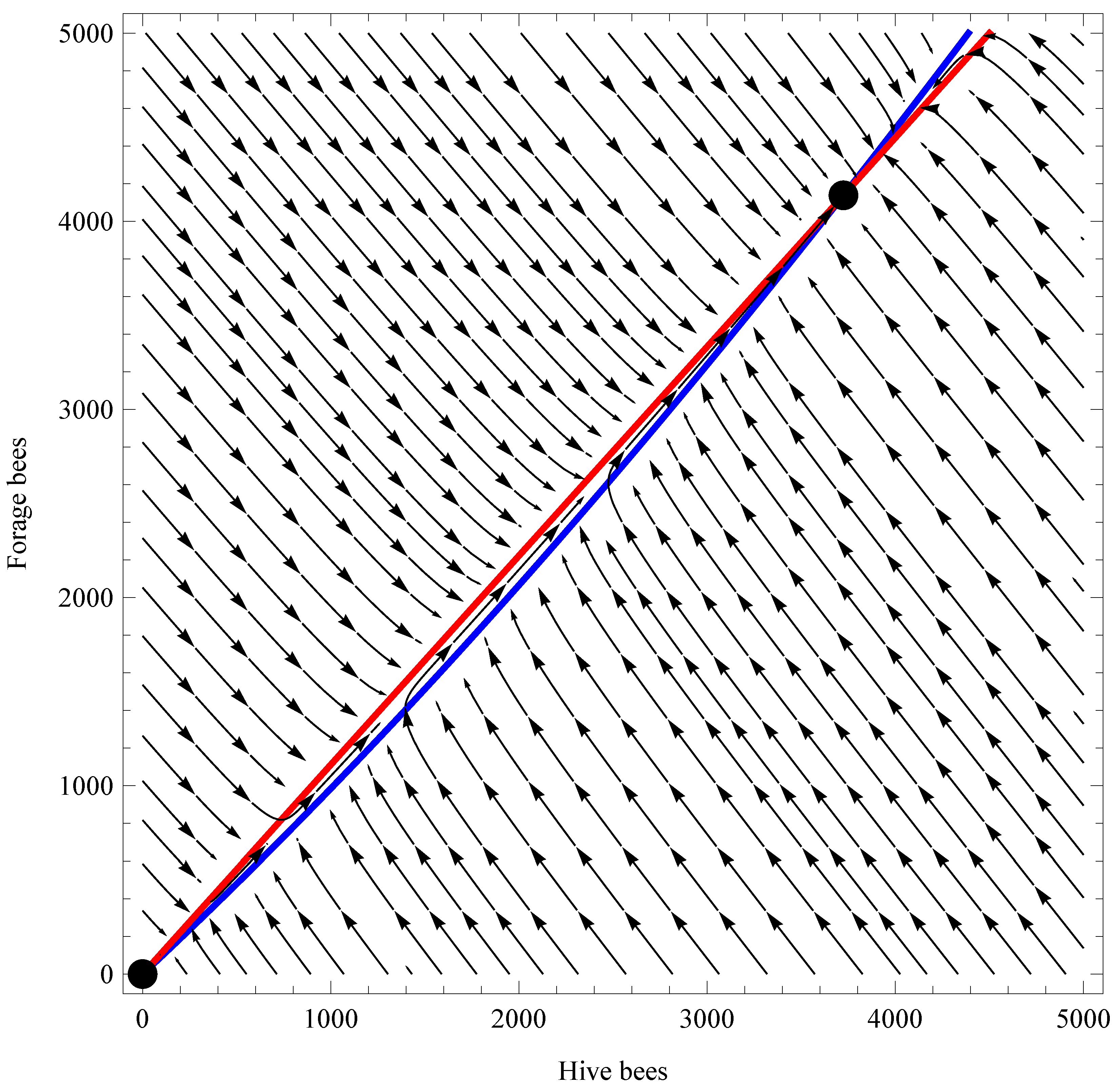
The results in Theorem 5 are illustrated in Figure 1 and Figure 2. In Figure 1, the model parameters are chosen as L = 2000 , w = 27000 , α = 0.25 , m = 0.2 , c = 0.5 , and d = 0.01 . From (13), it is easily calculated that R 0 0.8 . By Theorem 5, the trivial equilibrium E 0 = ( 0 , 0 ) is globally asymptotically stable in R + 2 .
In Figure 2, the parameters are set to L = 2000 , w = 27000 , α = 0.25 , m = 0.1 , c = 0.5 , and d = 0.01 . Note that the death rate of forager bees is smaller in this second parameter set compared to the first. Using (13), we find R 0 1.3 . According to Theorem 5, the trivial equilibrium E 0 is unstable, and there exists a unique positive equilibrium E 1 = ( H 1 , F 1 ) , which is globally asymptotically stable in R + 2 { E 0 } . Numerical computation yields H 1 3724 and F 1 4138 .
From the explicit expression in (13), it is clear that R 0 increases with L and decreases with both w and d. This behavior is biologically reasonable: a larger L or smaller w corresponds to a higher eclosion rate (see (9)), making colony persistence more likely. Conversely, a high death rate of hive bees, d, increases the risk of colony collapse. The influence of the parameters m, α , and c on R 0 is stated in the following proposition.
Proposition 2.
The basic reproduction number R 0 defined in (13) is an increasing function of the parameter L and a decreasing function of both parameters w and d. Furthermore, we have the following sensitivity results.
(a) 
If m > d , then R 0 decreases with α. If m < d , then R 0 increases with α. If m = d , then R 0 is independent of α.
(b) 
If m > d , then R 0 increases with c. If m < d , then R 0 decreases with c. If m = d , then R 0 is independent of c.
(c) 
As m increases, R 0 decreases.
(d) 
Denote β = α c . If m > d , then R 0 increases with β. If m < d , then R 0 decreases with β. If m = d , then R 0 is independent of β.
Proof. 
(a) Note from (13) that the following is obtained:
w ( d c + m ) L ( c + 1 ) R 0 = α + m / ( c + 1 ) α + d m / ( d c + m ) = 1 + m / ( c + 1 ) d m / ( d c + m ) α + d m / ( d c + m ) .
Since the following is valid:
m c + 1 d m d c + m = m ( m d ) ( c + 1 ) ( d c + m ) ,
we obtain
w ( d c + m ) L ( c + 1 ) R 0 α = m ( d m ) ( c + 1 ) ( d c + m ) [ α + d m / ( d c + m ) ] 2 .
Hence, the partial derivative R 0 / α has the same sign as d m . This proves (a).
(b) Similar as in the proof of (a), we rewrite (13) as follows:
w d R 0 L = c + ( m + α ) / α c + ( d m + m α ) / ( d α ) = 1 + ( m + α ) / α ( d m + m α ) / ( d α ) c + ( d m + m α ) / ( d α ) .
On account of the following:
m + α α d m + m α d α = 1 m d = d m d ,
we obtain (b).
(c) We again make use of (13) and obtain the following:
w ( d + α ) R 0 L = m + α c + α m + d α c / ( d + α ) .
Note that the following is obtained:
d α c d + α < α c < α c + α .
It is readily seen that R 0 is a decreasing function of m.
(d) Denote β = α c . It follows from (13) that the following is valid:
w d R 0 L = β + m + α β + m + m α / d = 1 + α ( 1 m / d ) β + m + m α / d .
Thus, the partial derivative R 0 / β has the same sign as m d . This proves (d). □
The biological interpretation of Proposition 2 is as follows. The mortalities of hive bees and forager bees (i.e., d and m, respectively) negatively affect R 0 . If m < d , meaning the death rate of forager bees is lower than that of hive bees, colony survival is promoted by a low hive-to-forager ratio c, together with a high hive-to-forager transition rate α and a low social inhibition rate α c . Conversely, if the death rate of forager bees exceeds that of hive bees ( m > d ), stronger social inhibition, combined with a low transition rate α and a high hive-to-forager ratio c, is more beneficial for the colony.

4. Conclusions

In this paper, we propose a general two-compartmental model to investigate the threshold dynamics of honey bee colonies. We explicitly derive the basic reproduction number R 0 as a critical threshold parameter, expressed in terms of the model parameters, and provide its biological interpretation. If R 0 < 1 , then the trivial equilibrium E 0 = ( 0 , 0 ) is locally asymptotically stable. If R 0 > 1 , then E 0 becomes unstable and the honey bee colony will persist. For the critical case R 0 = 1 , we make use of a general result in [14] and find the stability conditions for E 0 . Applications of our general results are demonstrated on a specific model incorporating commonly used functions for eclosion and social inhibition. We establish the global threshold dynamics for this system: the trivial equilibrium E 0 is globally asymptotically stable when R 0 1 , while the unique positive equilibrium is globally asymptotically stable when R 0 > 1 . A sensitivity analysis is performed to examine how the basic reproduction number is influenced by the model parameters, including the eclosion rate, the death rates of hive and forager bees, the social inhibition rate, and the hive-to-forager ratio.

5. Discussion

Our work has some limitations. The model we considered is monotone, and its dynamics are independent of the initial colony size. However, incorporating the Allee effect into the model [22] can lead to more complex behaviors, such as bistability. Our model includes only two compartments—hive bees and forager bees—while a more realistic approach would also account for brood dynamics [7]. In future work, we plan to investigate an age-structured model of honey bee colonies incorporating the Allee effect and the parasitic varroa mites [23]. In such a case, the trivial equilibrium should be unstable because a colony must maintain an adequate population of worker bees to provide brood care, thereby ensuring the sustained production of new individuals [24]. The maturation period of brood may play a crucial role in colony dynamics, potentially inducing Hopf bifurcations, and limit cycles. Seasonality plays a critical role in determining whether a colony persists or collapses. For instance, during winter, eclosion is greatly reduced and foraging activity ceases. Consequently, a switching periodic system offers a more realistic and meaningful framework than the autonomous system analyzed in this study. In addition, colonies in commercial beekeeping operations are often relocated. In forthcoming work, we intend to extend our analysis to a more general system that incorporates both periodicity and spatial movement. The model presented in this paper is deterministic, but it would be valuable to further investigate stochastic effects by incorporating random fluctuations in population size. While certain parameter regimes do not lead to colony collapse under the deterministic framework, the inclusion of stochasticity may change this outcome [25]. A natural extension of this study is to employ stochastic differential equations to capture vulnerabilities in colony survival that cannot be described by purely deterministic models.

Author Contributions

Conceptualization, X.-S.W.; Methodology, M.M.R. and X.-S.W.; Formal analysis, M.M.R.; Investigation, M.M.R. and X.-S.W.; Writing—original draft, M.M.R. and X.-S.W.; Writing—review & editing, X.-S.W.; Supervision, X.-S.W.; Project administration, X.-S.W.; Funding acquisition, X.-S.W. All authors have read and agreed to the published version of the manuscript.

Funding

This research was funded by the Louisiana Board of Regents Support Fund under contract No. LEQSF(2022-25)-RD-A-26.

Institutional Review Board Statement

Not applicable.

Informed Consent Statement

Not applicable.

Data Availability Statement

The original contributions presented in this study are included in the article. Further inquiries can be directed to the corresponding author.

Acknowledgments

We are deeply grateful to the anonymous referees for their careful reading and valuable suggestions, which have significantly improved this manuscript.

Conflicts of Interest

The authors declare no conflicts of interest.

References

  1. Evans, J.D.; Spivak, M. Socialized medicine: Individual and communal disease barriers in honey bees. J. Invertebr. Pathol. 2010, 103, S62–S72. [Google Scholar] [CrossRef]
  2. Ratnieks, F.L.W.; Carreck, N.L. Clarity on honey bee collapse? Science 2010, 327, 152–153. [Google Scholar] [CrossRef]
  3. Torres, D.J.; Ricoy, U.M.; Roybal, S. Modeling honey bee populations. PLoS ONE 2015, 10, e0130966. [Google Scholar] [CrossRef]
  4. Chen, J.; DeGrandi-Hoffman, G.; Ratti, V.; Kang, Y. Review on mathematical modeling of honeybee population dynamics. Math. Biosci. Eng. 2021, 18, 9606–9650. [Google Scholar] [CrossRef]
  5. USDA National Agricultural Statistics Service. Honey; USDA Economics, Statistics and Market Information System, Cornell University: Ithaca, NY, USA, 2025; Available online: https://usda.library.cornell.edu/concern/publications/hd76s004z (accessed on 12 September 2025).
  6. Russell, S.; Barron, A.B.; Harris, D. Dynamic modelling of honey bee (Apis mellifera) colony growth and failure. Ecol. Model. 2013, 265, 158–169. [Google Scholar] [CrossRef]
  7. Khoury, D.S.; Barron, A.B.; Myerscough, M.R. Modelling food and population dynamics in honey bee colonies. PLoS ONE 2013, 8, e59084. [Google Scholar] [CrossRef] [PubMed]
  8. Romero-Leiton, J.P.; Gutierrez, A.; Benavides, I.F.; Molina, O.E.; Pulgarín, A. An approach to the modeling of honey bee colonies. Web Ecol. 2022, 22, 7–19. [Google Scholar] [CrossRef]
  9. Amdam, G.V.; Omholt, S.W. The hive bee to forager transition in honeybee colonies: The double repressor hypothesis. J. Theor. Biol. 2003, 223, 451–464. [Google Scholar] [CrossRef]
  10. Huang, Z.; Robinson, G. Regulation of honey bee division of labor by colony age demography. Behav. Ecol. Sociobiol. 1996, 39, 147–158. [Google Scholar] [CrossRef]
  11. Varga, R.S. Matrix Iterative Analysis; Prentice-Hall: Englewood Cliffs, NJ, USA, 1962. [Google Scholar]
  12. Diekmann, O.; Heesterbeek, J.A.P.; Metz, J.A.J. On the definition and the computation of the basic reproduction ratio R0 in models for infectious diseases in heterogeneous populations. J. Math. Biol. 1990, 28, 365–382. [Google Scholar]
  13. van den Driessche, P.; Watmough, J. Reproduction numbers and sub-threshold endemic equilibria for compartmental models of disease transmission. Math. Biosci. 2002, 180, 29–48. [Google Scholar] [CrossRef]
  14. Mahbuba, J.E.; Wang, X.-S. Stability analysis of biological systems under threshold conditions. Symmetry 2025, 17, 1193. [Google Scholar] [CrossRef]
  15. Hale, J.K. Asymptotic Behavior of Dissipative Systems; American Mathematical Society: Providence, RI, USA, 1988. [Google Scholar]
  16. Smith, H.L.; Zhao, X.-Q. Robust persistence for semidynamical systems. Nonlinear Anal. 2001, 47, 6169–6179. [Google Scholar] [CrossRef]
  17. Magal, P.; Zhao, X.-Q. Global attractors and steady states for uniformly persistent dynamical systems. SIAM J. Math. Anal. 2005, 37, 251–275. [Google Scholar] [CrossRef]
  18. Hirsch, M.W. The dynamical systems approach to differential equations. Bull. Amer. Math. Soc. 1984, 11, 1–64. [Google Scholar] [CrossRef]
  19. Khoury, D.S.; Myerscough, M.R.; Barron, A.B. A quantitative model of honey bee colony population dynamics. PLoS ONE 2011, 6, e18491. [Google Scholar] [CrossRef] [PubMed]
  20. Booton, R.D.; Iwasa, Y.; Marshall, J.A.R.; Childs, D.Z. Stress-mediated Allee effects can cause the sudden collapse of honey bee colonies. J. Theor. Biol. 2017, 420, 213–219. [Google Scholar] [CrossRef] [PubMed]
  21. Elzinga, D.C.; Strickland, W.C. Generalized stressors on hive and forager bee colonies. Bull. Math. Biol. 2023, 85, 112. [Google Scholar] [CrossRef]
  22. Dennis, B.; Kemp, W.P. How hives collapse: Allee effects, ecological resilience, and the honey bee. PLoS ONE 2016, 11, e0150055. [Google Scholar]
  23. Britton, N.F.; White, K.A.J. The effect of covert and overt infections on disease dynamics in honey-bee colonies. Bull. Math. Biol. 2021, 83, 67. [Google Scholar] [CrossRef]
  24. Eberl, H.J.; Frederick, M.R.; Kevan, P.G. Importance of brood maintenance terms in simple models of the honeybee—Varroa destructor—Acute bee paralysis virus complex. Electron. J. Differ. Equ. 2010, 19, 85–98. [Google Scholar]
  25. Dynes, T.L.; Berry, J.A.; Delaplane, K.S.; Brosi, B.J.; de Roode, J.C. A model of infection in honeybee colonies with social immunity. PLoS ONE 2021, 16, e0247294. [Google Scholar]
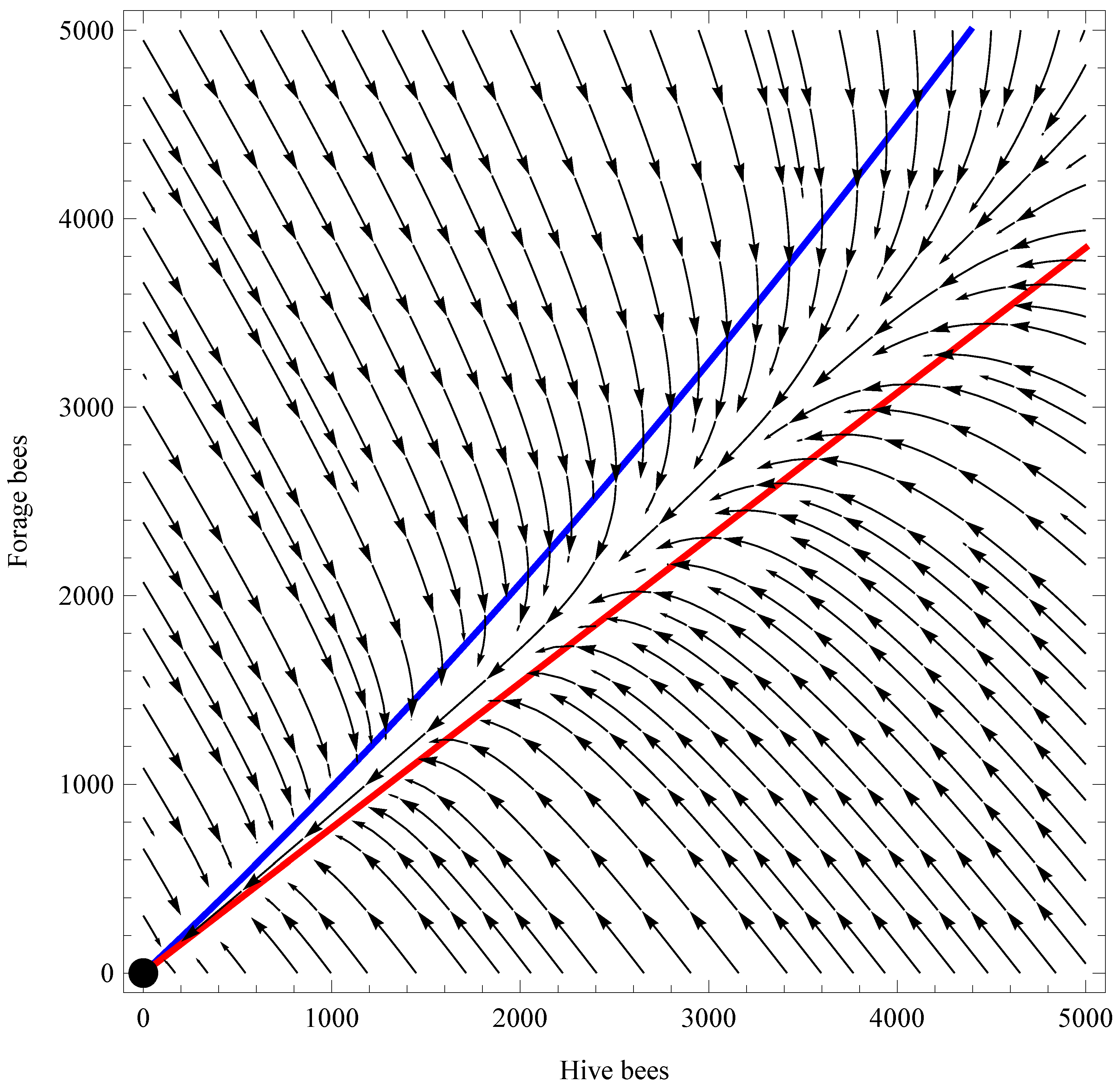
Figure 1. Phase portrait of system (11) and (12). The background arrows represent the vector field, indicating the direction of the ( H , F ) trajectories. The blue curve corresponds to the H-nullcline ( H = 0 ), and the red curve corresponds to the F-nullcline ( F = 0 ). Intersections of the nullclines (solid dots) indicate the equilibrium points of the system. The model parameters are chosen as L = 2000 , w = 27000 , α = 0.25 , m = 0.2 , c = 0.5 , d = 0.01 .
Axioms 14 00773 g001
Figure 2. Phase portrait of system (11) and (12). The background arrows represent the vector field, indicating the direction of the ( H , F ) trajectories. The blue curve corresponds to the H-nullcline ( H = 0 ), and the red curve corresponds to the F-nullcline ( F = 0 ). Intersections of the nullclines (solid dots) indicate the equilibrium points of the system. The model parameters are chosen as L = 2000 , w = 27000 , α = 0.25 , m = 0.1 , c = 0.5 , d = 0.01 .
Axioms 14 00773 g002
Disclaimer/Publisher’s Note: The statements, opinions and data contained in all publications are solely those of the individual author(s) and contributor(s) and not of MDPI and/or the editor(s). MDPI and/or the editor(s) disclaim responsibility for any injury to people or property resulting from any ideas, methods, instructions or products referred to in the content.