Abstract
In this manuscript, we propose a multi-step framework for solving nonlinear systems of algebraic equations. To improve the solver’s efficiency, the Jacobian matrix is held constant during the second sub-step, while a specialized strategy is applied in the third sub-step to maximize convergence speed without necessitating additional Jacobian evaluations. The proposed method achieves fifth-order convergence for simple roots, with its theoretical convergence established. Finally, computational experiments are conducted to illustrate the performance of the proposed solver in addressing nonlinear equation systems.
Keywords:
three-step method; fifth rate of convergence; Jacobian; Newton’s method; Fréchet derivative MSC:
41A25; 65H10
1. Preliminary Discussion
1.1. Nonlinear Equations
Nonlinear sets of equations are integral to numerous scientific and engineering applications, serving as fundamental tools in modeling and analysis [1,2,3,4]. These equations, due to their complexity, often defy exact analytical solutions (denoted by r), making their resolution an active area of research in applied mathematics. As a result, numerical iterative methods have become essential in approximating their solutions [5,6]. Iterative numerical methods play a vital role in resolving nonlinear sets of algebraic equations due to the inherent complexity and computational demands associated with such systems. The challenge becomes even more pronounced when dealing with high-dimensional systems where the number of equations and variables is substantial. Iterative methods provide a systematic approach to approximate the solution of nonlinear systems through successive refinements, enabling the computation of accurate results with manageable computational resources. Their ability to converge towards a solution makes iterative techniques indispensable in numerical analysis [7,8,9].
1.2. The Need in Differential Equations
Nonlinear partial differential equations (PDEs) [10,11] frequently arise in diverse scientific and engineering fields, such as fluid mechanics. These equations are generally challenging to solve analytically due to the lack of closed-form solutions, requiring the development and application of numerical solvers. One common approach involves discretizing the continuous problem using methods like finite difference (FD), which reformulates the PDE into a set of nonlinear algebraic equations. To tackle such resulting systems efficiently, advanced iterative solvers, such as the higher-order methods furnished in this study, can be employed. These solvers utilize higher-order procedures and exploit enhanced convergence features to provide fast and efficient solutions while substantially reducing calculational effort compared to conventional approaches.
Higher-order iterative solvers for solving nonlinear PDEs consist of several crucial stages. The process begins with discretizing the PDE, converting it into a large and often sparse nonlinear algebraic system. Subsequently, an initial approximation for the solution is provided, serving as a starting point for the iterative refinement.
Another advantage of iterative methods is their scalability to large-dimensional problems [12]. Consider, for instance, a system of nonlinear equations arising from modeling a three-dimensional fluid dynamics problem, such as simulating airflow over an aircraft. Such systems can involve millions of variables and equations derived from discretizing PDEs governing fluid flow. Iterative methods, on the other hand, decompose the problem into smaller, more manageable steps. By iteratively improving the solution starting from an initial guess, these methods can efficiently handle large systems while taking advantage of sparsity and other problem-specific structures to reduce computational overhead (see [13] for more).
1.3. Our Aim and Contribution
This study is driven by the necessity to develop a robust iterative framework that emphasizes computational efficiency and precision. By drawing on foundational ideas from prior research [14,15], our approach introduces a strategy that circumvents the need for second-order Fréchet derivative calculations. This not only simplifies the computational process but also contributes to advancing numerical methodologies in the field. The core aim is to design a solver capable of handling both real and complex roots, achieving high convergence rates while minimizing computational demands such as matrix inversions and function evaluations. To enhance the solver’s efficiency, the Jacobian matrix is frozen during the second sub-step, while a strategy is employed in the third sub-step to maximize convergence speed without requiring additional Jacobian computations. This approach achieves a fifth-order convergence rate for simple roots, and its theoretical convergence has been rigorously analyzed.
1.4. Existing Approaches
The problem under consideration is formulated as follows [16,17]:
where
and , are component functions defined over a convex domain . To build on the current state of knowledge, we revisit and assess several classical iterative methods for solving (1).
One widely studied technique is Newton’s method (NM), which operates as follows [18,19]:
NM is well known for its quadratic convergence rate, provided the initial vector lies sufficiently near to the simple zero. Nevertheless, its reliance on Jacobian computations can pose challenges, leading to the development of alternative methods.
It is noted that iterative methods provide flexibility in handling systems with nonlinearity and lack of symmetry, which are common in practical applications. For example, nonlinear systems often arise in optimization, structural engineering, and machine learning, where the governing equations are complex and highly sensitive to initial conditions. Iterative approaches, such as Newton’s solver and its other alternatives, can adapt to these challenges. This adaptability ensures that iterative methods remain effective across a wide spectrum of applications, making them an essential tool in computational mathematics.
Derivative-free techniques such as Steffensen’s method (SM) have been proposed as follows [20]:
where the divided difference operator (DDO) is central to its implementation. For vectors and z, the DDO is defined as:
The author in [6] furnished an improvement to the NM that reaches local third order (here abbreviated as TM) as follows:
Despite the utility of the above methods, certain drawbacks persist, such as the formation of dense matrices during DDO computations, which limit their scalability to large systems.
1.5. Outlines
Motivated by these challenges, this manuscript proposes an innovative multistep solver with fifth-order convergence rates. The solver is particularly designed to eliminate the need for second-order Fréchet derivatives. The structure of the manuscript is given as follows. Section 2 introduces the design of a proposed multistep solver, highlighting its computational efficiency through reduced LU decompositions. Section 3 presents a detailed theoretical error analysis to confirm the convergence properties. Section 4 applies the presented solver to benchmark test cases. Section 5 concludes with a summary of observations and suggests potential directions for future investigations.
2. A Novel Iterative Framework
This section introduces a refined iterative methodology derived from the foundational techniques outlined in Section 1. The proposed scheme utilizes multiple steps while maintaining a fixed Jacobian matrix to achieve improved computational performance. We first consider the the following three-step strategy:
Evidently, (6) is a three-step structure of (2) and reaches the eighth order of convergence, but requires Jacobian computation three times and makes no meaningful advance in contrast to (2). To improve this, we follow the Traub’s idea in (5) and consider a frozen structure as follows:
The scheme (8) is not that useful since it follows (5) and reaches only the fourth convergence speed. To furnish a useful technique, a DDO is designed carefully in the third substep. For such a target, we first consider:
where for the sake of simplicity in the scalar case, the DDO1 is given by:
Here, and are two appropriate parameters that must be set using the knowledge of the previous substeps to gain as must possible of convergence order. We choose:
Since the Jacobian has already been computed in the first substep, it does not add extra new functional or derivative evaluations to the structure of the proposed method. Hence, the final formulation is expressed as follows (CS5):
In practical computations, direct matrix inversion is computationally expensive and should be avoided. Instead, LU decomposition is employed to solve the associated linear systems. Consequently, during the implementation of CS5, several distinct linear systems are solved at each iteration to estimate the resolution of the nonlinear problem (1):
Rewriting the iterative schemes for practical implementation, CS5 is reformulated as:
This acceleration improves computational efficiency, particularly for complex and high-dimensional problems. The efficiency of a numerical algorithm is a cornerstone of computational mathematics, dictated by its convergence rate and structural design relative to computational costs. The quality of a solver is evaluated based on these factors, considering the number of function evaluations, Jacobian computations, and LU decompositions. This will be discussed later at the beginning of Section 4.
3. Investigating the Convergence Rate
Here, we conduct a convergence analysis to determine the convergence rates of the solver (13), or equivalently (11). Before presenting the main analytical order, the N-D Taylor series is furnished. The convergence rate for the solver CS5 is derived using the N-dimensional Taylor series. Let show the error at the -th loop. As detailed in [21], the following relationship holds:
where F exhibits the properties of a p-linear map, and . Additionally, the following holds:
Assuming that is Fréchet differentiable over D [22], the m-th derivative of H at for can be expressed as an m-linear map, i.e.,
such that . For near r, the Taylor series expansion is given by [22]:
wherein
It follows that and . Moreover, for , the following expansion holds:
whereas I is the unit matrix, and .
Theorem 1.
Let be suitably smooth in the Fréchet sense at each node in D, and suppose at some . Furthermore, assume that is smooth and invertible at r. Then, the sequence via CS5 locally tends to r with 5th-rate.
Proof.
To establish the convergence rate, we use the expansions from (17) and (19) to obtain the following expressions:
and
where for , and . Using these expansions, we derive:
A similar Taylor expansion using (20)–(22) gives the error at the end of the second sub-step of CS5 as follows:
Subsequently, we obtain:
By employing these expressions in the 3rd sub-step of CS5, we obtain:
which demonstrates that the method achieves a fifth-order, requiring only two LU decompositions for every iterates. This completes the proof. □
4. Numerical Tests
The primary objective here is to demonstrate the applicability and efficacy of the proposed CS5 scheme. Some remarks are given as:
- Computational experiments were performed using Wolfram software 13.3 [23,24], with all programming conducted in a multiple-precision arithmetic framework using 2500-digit precision except the last test. This setup allowed us to rigorously observe and verify the higher speeds reflected in the computational pieces of evidence.
- Linear systems arising during the process were efficiently solved through LU factorization using .
- All numerical tests were carried out in a consistent computational environment to ensure reliability and reproducibility.
- For comparative analysis, the proposed higher-order method was benchmarked against existing approaches, including NM and SM, for resolving nonlinear collections of equations.
Prior to presenting the numerical results, we highlight the efficiency indices (EI) of the solvers under comparison. Attaining fifth-order convergence with the CS5 scheme requires solving three linear systems per iteration cycle. However, computational efficiency is enhanced by requiring only two LU factorizations per cycle, followed by matrix-vector multiplications, thereby eliminating the need for repeated matrix inversions within each iteration. The efficiency index, as defined in [20], is calculated as:
whereas
- shows the cost, and
- shows the rate in terms of function evaluations.
For evaluating the EI of the CS5 scheme, we detail the required functional evaluation costs in -dimensional functions and their Jacobians as follows: For , evaluations are required for each. For , evaluations are needed. Similarly, for the divided difference operator (DDO1), evaluations are also involved.
The results summarized in Table 1 clearly show that when changing , the EI of the proposed solver surpasses that of its competitors. A comparative analysis of different solvers, visualized in Figure 1, underscores the superiority of the CS5 scheme.

Table 1.
Comparison of various techniques based on their efficiency indices.
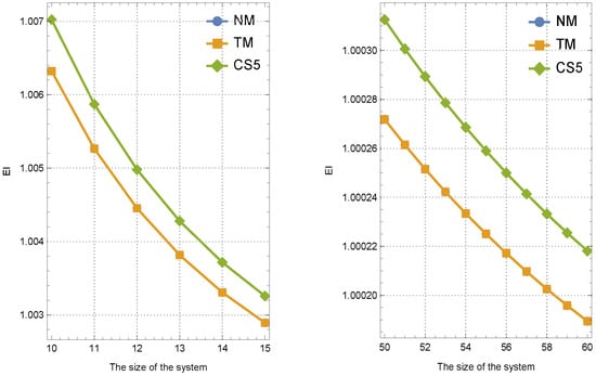
Figure 1.
Evaluation of EIs for different values of .
Example 1.
The nonlinear set , which encompasses a real root, is analyzed in detail as described in the following
where its simple root is:
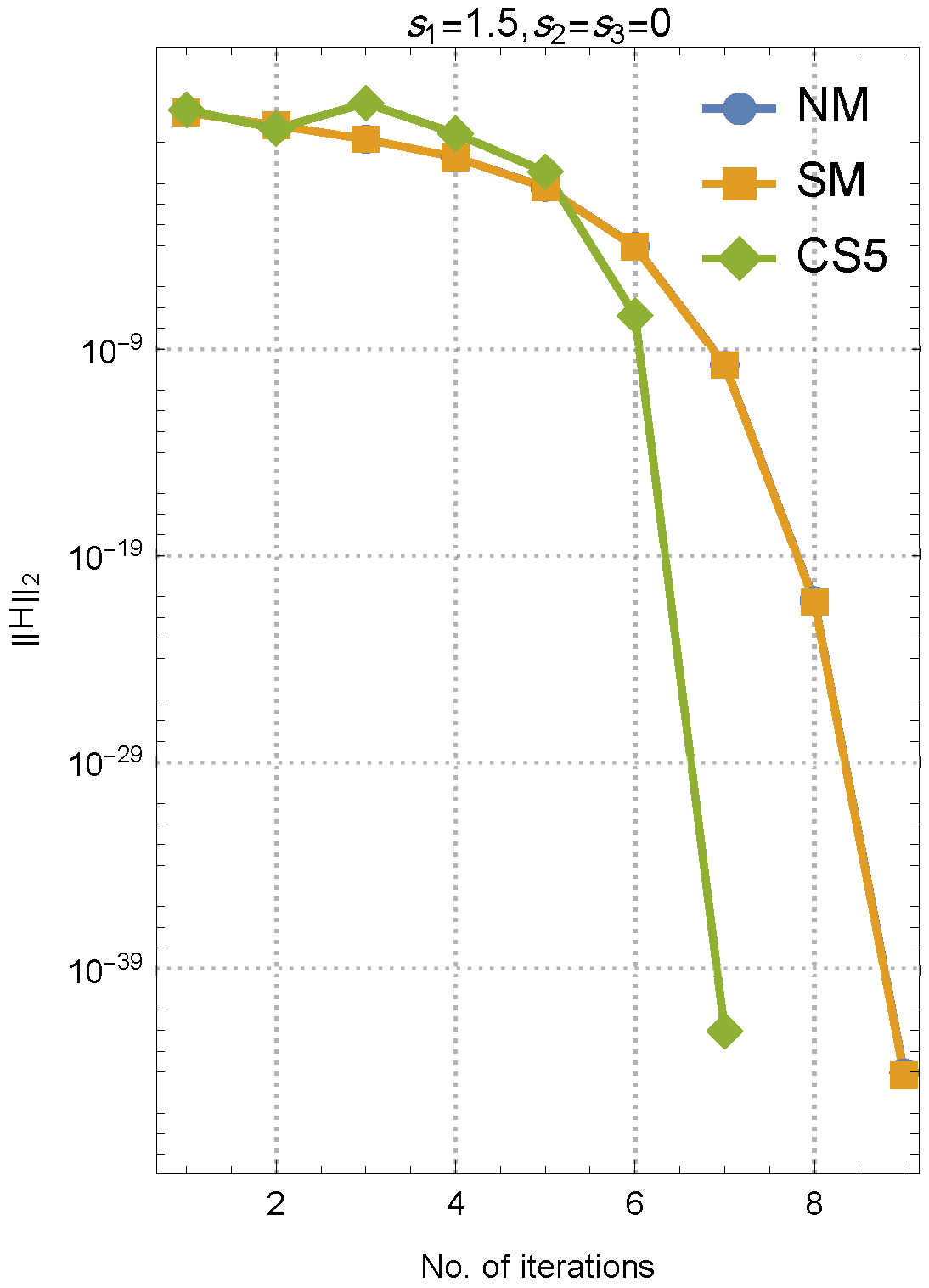
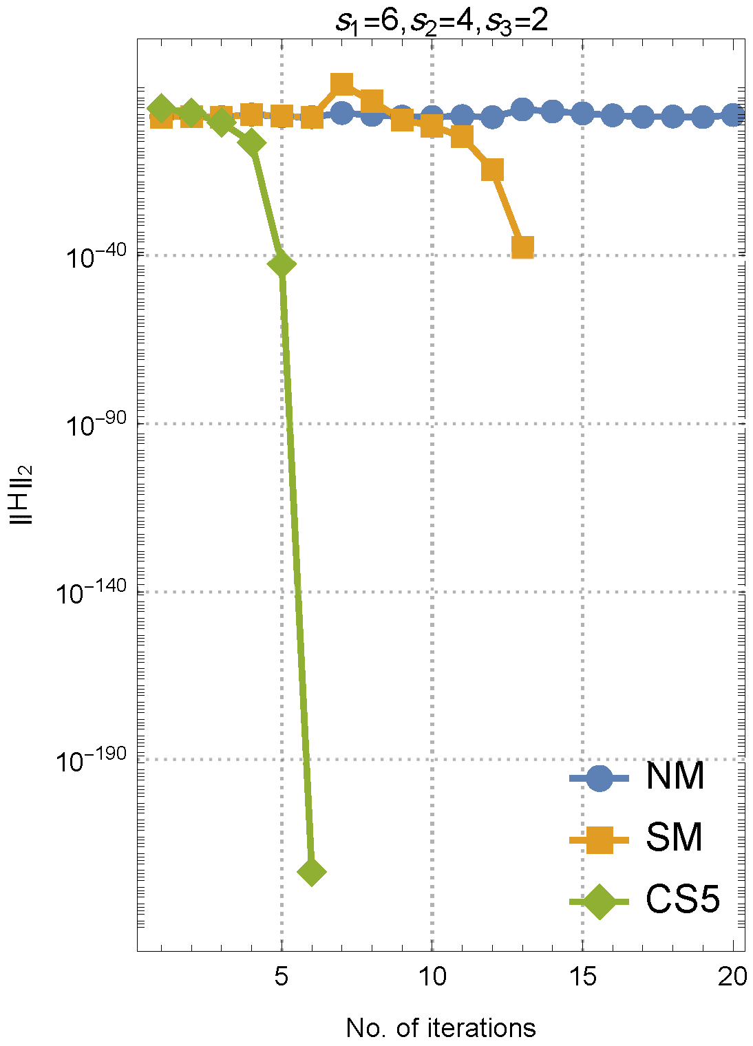
The computational results are presented in Figure 2, Figure 3 and Figure 4. Here, different starting points have been compared for any of the figures to reveal the usefulness of the new method. Furthermore, the norm of residual is expressed through the use of the notation, providing a concise representation of the error magnitude.

Figure 2.
Results of comparions for different solvers under . Here, NM and SM coincide very much with each other.
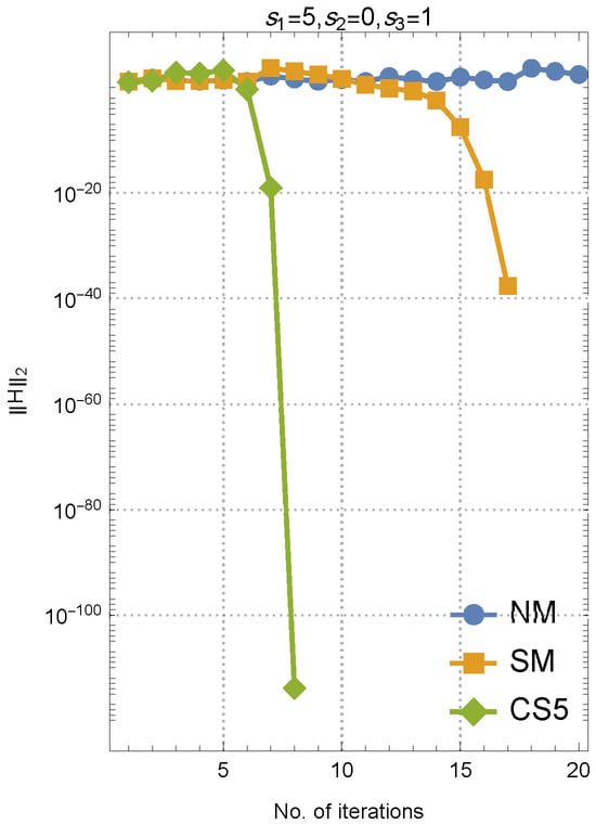
Figure 3.
Results of comparisons for different solvers under .

Figure 4.
Results of comparisons for different solvers under .
A simple yet effective implementation for CS5 in Example 1 has now been provided in the Mathematica environment to make the process easier for readers as follows (noting that the notations may not be necessarily the same as the mathematical notations in the derivation of the method):
ClearAll["Global‘*"];
digits = 2500; size = 3;
f[{x1_, x2_, x3_}] :=
{
Sin[x1 + x2 - x3],
Cos[x1 - x2],
x1^2 + x2^2 - x3
};
J[{x1_, x2_, x3_}] = D[f[{x1, x2, x3}], {{x1, x2, x3}}];
x = SetAccuracy[{6, 4, 2}, digits];
max = 6; fx = f[x];
point1[j_] := Join[x1[[;; j]], w[[j + 1 ;;]]];
point2[j_] := Join[x1[[;; j - 1]], w[[j ;;]]];
Do[{
f1x = J[x];
yy = LinearSolve[f1x];
w = x - yy[fx];
fw = f[w];
x1 = w - yy[fw];
fx1 = f[x1];
T = Transpose@
SparseArray@
Table[(f[point1[j]] - f[point2[j]])/(x1[[j]] - w[[j]]), {j,
size}];
fun = LinearSolve[T];
x = x1 - fun[(fx1)];
fx = f[x];
L[i] = Norm[fx, 2];
}, {i, 1, max}
]; // AbsoluteTiming
s3 = Table[N[L[k], 5], {k, 1, max}]
N[x, 5]
Example 2.
The performance and accuracy of the presented scheme is validated by solving the following nonlinear test problem: , where . The function H is defined as:
The iterative process begins with the initial vector , with the objective of converging to the exact solution .
Numerical experiments, presented in Table 2, highlight the robustness of the proposed scheme in solving a variety of nonlinear equations. These computational tests reveal that the CS5 scheme converges to the solutions in only a few iterations while delivering high accuracy at every iterate. Furthermore, the numerical rate consistently aligns with the analytically expected higher speeds, confirming the reliability and efficiency of the method.
Table 2.
A presentation of the numerical outcomes obtained from the application of various methods in Example 2.
Example 3.
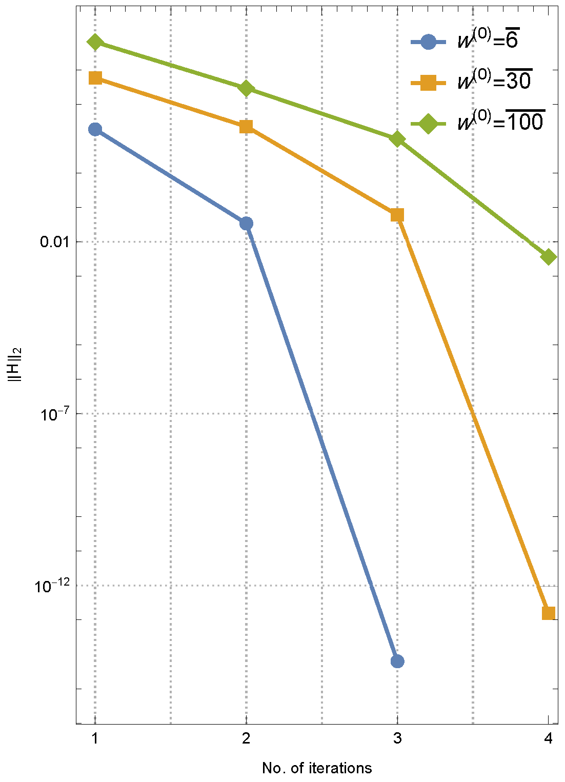
To have a test problem of higher dimensions, we take into account
in which the simple root is for odd N. Here we test the performance of CS5 for in three different initial guesses.
The results for this problem are illustrated in Figure 5, re-verifying the effectiveness of the proposed procedure for higher dimensional test problems. The fast convergence for CS5 in machine precision can be observed for all the considered initial guesses.
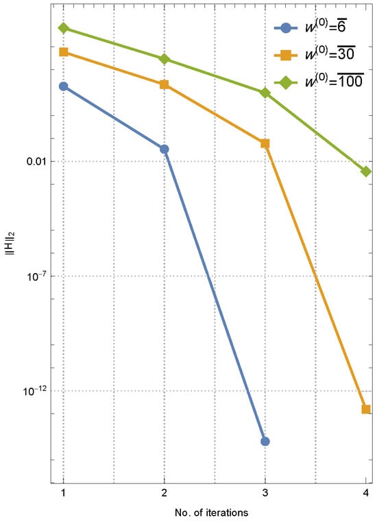
Figure 5.
Results of comparisons for different initial approximations using CS5 in Example 3.
Discussion
In this section, we illustrate the performance of the proposed solver, CS5, in solving systems of nonlinear equations. Our observations indicate that the CS5 scheme demonstrates rapid convergence for both low-dimensional and high-dimensional systems. Moreover, in several cases, it exhibits a superior convergence radius compared to classical methods such as the NM and the SM. The proposed scheme comprises three steps, utilizing a single Jacobian matrix for the first two steps and a DDO in the final sub-step to achieve local fifth-order convergence.
5. Summary
In this work, we have introduced and analyzed a novel iteration solver aimed at resolving collections of nonlinear equations efficiently and accurately. Building upon existing techniques, we have furnished an enhanced multi-step scheme, denoted as CS5, that incorporates fixed Jacobian approximations to balance computational cost and convergence performance. Through careful design and theoretical underpinnings, these method has demonstrated fifth-order convergence, achieving higher efficiency while requiring fewer computations per iteration compared to traditional approaches. The analysis has relied on the Taylor series expansion and Frèchet differentiability, which have provided the foundation for establishing convergence rates.
Throughout this study, we have emphasized the balance between computational efficiency and accuracy, showcasing that our methods align well with the principles of numerical optimization. The proposed iterative schemes not only reduce the need for matrix inversion by adopting LU decomposition techniques but also maintain a high degree of flexibility in practical implementation. This balance ensures their suitability for a wide range of nonlinear problems, making them valuable tools in computational mathematics. We have demonstrated the capacity of a fifth-order iterative method to offer competitive solutions despite the existence of higher-order methods. By strategically freezing or updating the derivative operator at critical stages, our method has exhibited the ability to expand the convergence domain while maintaining simplicity and practical relevance. Future directions might be focused on several aspects. First, it is of theoretical interest to investigate how freezing the DDO at the third substep for CS5 can impact the convergence order when it is frozen an arbitrary multi-step format. Additionally, studying the semi local convergence of the scheme in order to relax the assumption of the smoothness of the function can be investigated further.
Author Contributions
Conceptualization, M.L.; Methodology, M.L.; Formal analysis, M.L.; Investigation, S.S.; Writing—original draft, M.L.; Writing—review & editing, S.S.; Visualization, S.S.; Supervision, S.S.; Funding acquisition, S.S. All writers equally contributed to this paper. All authors have read and agreed to the published version of the manuscript.
Funding
This research received no external funding.
Data Availability Statement
The findings and contributions outlined in this research are documented within the manuscript. Any additional questions or requests for clarification may be addressed by reaching out to the corresponding author.
Conflicts of Interest
The writers state that they have no conflicts of interest.
References
- Soheili, A.R.; Amini, M.; Soleymani, F. A family of Chaplygin–type solvers for Itô stochastic differential equations. Appl. Math. Comput. 2019, 340, 296–304. [Google Scholar] [CrossRef]
- Behl, R. A derivative free fourth-order optimal scheme for applied science problems. Mathematics 2022, 10, 1372. [Google Scholar] [CrossRef]
- Gdawiec, K.; Kotarski, W.; Lisowska, A. Visual analysis of the Newton’s method with fractional order derivatives. Symmetry 2019, 11, 1143. [Google Scholar] [CrossRef]
- Chanu, W.H.; Panday, S.; Thangkhenpau, G. Development of optimal iterative methods with their applications and basins of attraction. Symmetry 2022, 14, 2020. [Google Scholar] [CrossRef]
- Ortega, J.M.; Rheinboldt, W.C. Iterative Solutions of Nonlinear Equations in Several Variables; Academic Press: New York, NY, USA, 1970. [Google Scholar]
- Traub, J. Iterative Methods for the Solution of Equations, 2nd ed.; Chelsea Publishing Company: New York, NY, USA, 1982. [Google Scholar]
- Wang, X.; Zhang, T.; Qin, Y. Efficient two-step derivative-free iterative methods with memory and their dynamics. Int. J. Comput. Math. 2016, 93, 1423–1446. [Google Scholar] [CrossRef]
- Proinov, P.D. New general convergence theory for iterative processes and its applications to Newton-Kantorovich type theorems. J. Complex. 2010, 26, 3–42. [Google Scholar] [CrossRef]
- Ivanov, S.I. A general approach to the study of the convergence of Picard iteration with an application to Halley’s method for multiple zeros of analytic functions. J. Math. Anal. Appl. 2022, 513, 126238. [Google Scholar] [CrossRef]
- Qasim, S.; Ali, S.; Ahmad, F.; Serra-Capizzano, S.; Ullah, M.Z.; Mahmood, A. Solving systems of nonlinear equations when the nonlinearity is expensive. Comput. Math. Appl. 2016, 71, 1464–1478. [Google Scholar] [CrossRef]
- Soheili, A.R.; Soleymani, F. Iterative methods for nonlinear systems associated with finite difference approach in stochastic differential equations. Numer. Algorithms 2016, 71, 89–102. [Google Scholar] [CrossRef]
- Cordero, A.; Jordán, C.; Sanabria-Codesal, E.; Torregrosa, J.R. Solving nonlinear vectorial problems with a stable class of Jacobian-free iterative processes. J. Appl. Math. Comput. 2024, 70, 5023–5048. [Google Scholar] [CrossRef]
- Shil, S.; Nashine, H.K.; Soleymani, F. On an inversion-free algorithm for the nonlinear matrix problem Xα + A*X−βA + B*X−γB = I. Int. J. Comput. Math. 2022, 99, 2555–2567. [Google Scholar] [CrossRef]
- Abdullah, S.; Choubey, N.; Dara, S. An efficient two-point iterative method with memory for solving non-linear equations and its dynamics. J. Appl. Math. Comput. 2023, 70, 285–315. [Google Scholar] [CrossRef]
- Cordero, A.; Garrido, N.; Torregrosa, J.R.; Triguero-Navarro, P. Design of iterative methods with memory for solving nonlinear systems. Math. Method. Appl. Sci. 2023, 46, 12361–12377. [Google Scholar] [CrossRef]
- Batra, P. Simultaneous point estimates for Newton’s method. BIT 2002, 42, 467–476. [Google Scholar] [CrossRef]
- McNamee, J.M.; Pan, V.Y. Numerical Methods for Roots of Polynomials—Part I; Elsevier: Amsterdam, The Netherlands, 2007. [Google Scholar]
- Kyncheva, V.K.; Yotov, V.V.; Ivanov, S.I. Convergence of Newton, Halley and Chebyshev iterative methods as methods for simultaneous determination of multiple polynomial zeros. Appl. Numer. Math. 2017, 112, 146–154. [Google Scholar] [CrossRef]
- McNamee, J.M.; Pan, V.Y. Numerical Methods for Roots of Polynomials—Part II; Elsevier: Amsterdam, The Netherlands, 2013. [Google Scholar]
- Grau-Sánchez, M.; Grau, À.; Noguera, M. On the computational efficiency index and some iterative methods for solving systems of nonlinear equations. J. Comput. Appl. Math. 2011, 236, 1259–1266. [Google Scholar] [CrossRef]
- Sharma, J.R.; Guha, R.K.; Sharma, R. An efficient fourth order weighted-Newton method for systems of nonlinear equations. Numer. Algorithms 2013, 62, 307–323. [Google Scholar] [CrossRef]
- Cordero, A.; Hueso, J.L.; Martínez, E.; Torregrosa, J.R. A modified Newton-Jarratt’s composition. Numer. Algorithms 2010, 55, 87–99. [Google Scholar] [CrossRef]
- Dubin, D. Numerical and Analytical Methods for Scientists and Engineers Using Mathematica; John Wiley & Sons: Hoboken, NJ, USA, 2003. [Google Scholar]
- Clark, J.; Kapadia, D. Introduction to Calculus: A Computational Approach; Wolfram Media: Champaign, IL, USA, 2024. [Google Scholar]

Disclaimer/Publisher’s Note: The statements, opinions and data contained in all publications are solely those of the individual author(s) and contributor(s) and not of MDPI and/or the editor(s). MDPI and/or the editor(s) disclaim responsibility for any injury to people or property resulting from any ideas, methods, instructions or products referred to in the content. |
© 2025 by the authors. Licensee MDPI, Basel, Switzerland. This article is an open access article distributed under the terms and conditions of the Creative Commons Attribution (CC BY) license (https://creativecommons.org/licenses/by/4.0/).