Bifurcation and Dynamics Analysis of a Piecewise-Linear van der Pol Equation

Abstract

In this study, we examine the bifurcations and dynamics of a piecewise linear van der Pol equation—a model that captures self-sustained oscillations and is applied in various scientific disciplines, including electronics, neuroscience, biology, and economics. The van der Pol equation is transformed into a piecewise linear system to simplify the analysis of stability and controllability, which is particularly beneficial in engineering applications. This work explores the impact of increasing the number of linear segments on the system’s dynamics, focusing on the stability of the equilibria, phase portraits, and bifurcations. The findings reveal that while the bifurcation structure at critical values of the bifurcation parameter is complex, the topology of the piecewise linear model remains unaffected by an increase in the number of linear segments from three to four. This research contributes to our understanding of the dynamics of nonlinear systems with piecewise linear characteristics and has implications for the analysis and design of real-world systems exhibiting such behavior.

1. Introduction

The van der Pol (VDP) equation is a second-order nonlinear differential equation that is widely used to model self-sustained oscillations in various systems. Originally, it was formulated to describe the behavior of electrical circuits involving vacuum tubes; however, the VDP equation has now found application across multiple scientific disciplines. The standard form of the VDP equation is given by

$$ϵv^{″}+(v^2-1)v^{\prime }+v-\lambda =0,$$

(1)

where ${\displaystyle v^{\prime }=\frac{dv}{dt}}$, v represents the displacement, t denotes the time, $\lambda$ is a bifurcation parameter, and $0<ϵ\ll 1$. This equation is particularly useful in modeling nonlinear dynamical systems, such as electronic circuits, where it aids in understanding their stability and oscillatory behavior [1].

The VDP equation has been extended in various ways to capture more complex dynamics. For instance, King and Gaito [2] introduced the autonomous van der Pol–Duffing (ADVP) oscillator, which incorporated a cubic nonlinear term to describe richer dynamical behaviors, including bistability. Further modifications by Matouk and Agiza [3] led to the development of the modified autonomous van der Pol–Duffing (MADVP) circuit, which included additional nonlinear terms, enabling the study of more complex phenomena, such as bifurcations and chaos [4]. Beyond electronics, the VDP equation has been applied in neuroscience to modeling neural excitability and spiking behaviors [5]; in biology to studying rhythmic processes such as heartbeats [6]; and in fields such as plasma physics [7], economics [8], and mechanical engineering [9].

Numerous methods have been developed for solving the VDP equation and its variants, including the Krylov–Bogoliubov–Mitropolsky technique [10], the residual harmonic balance method [11], the iteration method [12], the homotopy analysis method [13], and the modified Adomian decomposition method [14].

Despite the versatility of the VDP equation, its nonlinear nature often complicates analyses, particularly when the primary focus is on stability and controllability, rather than the detailed behavior of nonlinearities. In such cases, a piecewise linear (PWL) approximation of the VDP equation can offer a more suitable alternative. Through replacing the nonlinear terms with linear segments, the system’s complexity can be reduced, allowing for the application of well-established linear analysis techniques. This approach is particularly advantageous in engineering applications, where the ability to model and efficiently analyze system behaviors is crucial [15,16].

The motivation for the employment of PWL approximations arises from the work of Desroches et al. [17] and Rotstein et al. [18], who explored Liénard systems and FitzHugh–Nagumo models with multiple linear zones. These studies demonstrated that PWL systems can effectively capture the adaptive behavior of systems that exhibit different dynamics under varying conditions. By dividing the system into linear segments, the PWL approach enables the use of linear analysis tools to study stability, bifurcations, and other dynamical properties in each segment. This method has been successfully applied to various models, including the VDP equation, to analyze phenomena such as canard explosions and limit cycles [16,18,19,20,21,22,23,24,25,26,27,28].

In this work, we extend the PWL approach by constructing a four-zone PWL VDP equation and comparing its topological properties with those of a three-zone PWL VDP system. The idea of increasing the number of linear segments from three to four is motivated by the need to capture more nuanced dynamical behaviors that may not be adequately represented by fewer segments. Previous studies on three-zone PWL VDP systems have provided significant insights into the existence and uniqueness of limit cycles, as well as the occurrence of canard phenomena [21,22,23]. However, these studies have not explored the effects of varying the number of linear segments on the system’s overall dynamics. By increasing the number of segments, we aim to facilitate a more comprehensive understanding of the ways in which the topologies of PWL systems evolve with increasing complexity.

The structure of this paper is as follows. In Section 2, we present the necessary definitions and theorems for our analysis. Section 3 introduces the four-zone PWL VDP equation and discusses the stability of the equilibria, phase portraits, and bifurcations. In Section 4, we compare the results obtained from the four-zone system with those of the three-zone PWL VDP equation. Finally, Section 5 summarizes the main findings of this study and discusses future research directions.

2. Preliminaries

A system that is smooth and continuous in a piecewise manner on a plane, dependent on a parameter denoted by $\mu$, can be expressed in the form

$$\dot{\mathit{x}}=\left\{\begin{array}{cc}{\mathit{G}}_{\mathbf{1}}(\mathit{x},\mu ),\hfill & \mathrm{when}K(\mathit{x},\mu )<0,\hfill \\ {\mathit{G}}_{\mathbf{2}}(\mathit{x},\mu ),\hfill & \mathrm{when}K(\mathit{x},\mu )>0,\hfill \end{array}\right.$$

(2)

where ${\displaystyle \dot{\mathit{x}}=\frac{d\mathit{x}}{dt}}$, $\mathit{x}=(x,y)\in \mathcal{C}\subset {\mathbb{R}}^2$. This system is characterized by two distinct functions, ${\mathit{G}}_{\mathbf{1}}$ and ${\mathit{G}}_{\mathbf{2}}$, which are smooth and map from ${\mathbb{R}}^3$ to ${\mathbb{R}}^2$. The transition between these two functions ${\mathit{G}}_{\mathbf{1}}$ and ${\mathit{G}}_{\mathbf{2}}$ is governed by the condition $K(\mathit{x},\mu )=0$, which serves as the boundary of discontinuity, denoted by $\mathsf{\Sigma }$. Note that K is smooth and maps from ${\mathbb{R}}^3$ to $\mathbb{R}$. This boundary divides the domain $\mathcal{C}$ into two distinct regions, $D_1$ and $D_2$, where

• $D_1$ includes all points $\mathit{x}$ in $\mathcal{C}$ for which $K(\mathit{x},\mu )$ is less than zero;
• $D_2$ includes all points $\mathit{x}$ in $\mathcal{C}$ for which $K(\mathit{x},\mu )$ is greater than zero.

Under the assumption of continuity, we define

$${\mathit{G}}_{\mathbf{2}}(\mathit{x},\mu )={\mathit{G}}_{\mathbf{1}}(\mathit{x},\mu )+\mathit{J}(\mathit{x},\mu )K(\mathit{x},\mu ),$$

(3)

where $\mathit{J}(\mathit{x},\mu ):{\mathbb{R}}^3\mapsto {\mathbb{R}}^2$ is smooth. This ensures that ${\mathit{G}}_{\mathbf{1}}(\mathit{x},\mu )$ and ${\mathit{G}}_{\mathbf{2}}(\mathit{x},\mu )$ are identical when $K(\mathit{x},\mu )$ equals zero, in line with the requirement for a continuous transition.

 Definition 1 

(Admissible equilibrium [29]). We designate a point $\mathit{x}$ within the domain $\mathcal{C}$ as an admissible equilibrium for system (2) if it meets one of the following conditions:

 1. 

${\mathit{G}}_{\mathbf{1}}(\mathit{x},\mu )=0$ and $K(\mathit{x},\mu )$ is less than zero;

 2. 

${\mathit{G}}_{\mathbf{2}}(\mathit{x},\mu )=0$ and $K(\mathit{x},\mu )$ is greater than zero.

 Definition 2 

(Virtual equilibrium [29]). A point $\overline{\mathit{x}}$ within the domain $\mathcal{C}$ is referred to as a virtual equilibrium for system (2) under one of the following circumstances:

 1. 

${\mathit{G}}_{\mathbf{1}}(\overline{\mathit{x}},\mu )=0$ while $K(\overline{\mathit{x}},\mu )$ is greater than zero;

 2. 

${\mathit{G}}_{\mathbf{2}}(\overline{\mathit{x}},\mu )=0$ while $K(\overline{\mathit{x}},\mu )$ is less than zero.

 Definition 3 

(Boundary equilibrium [29]). We define a point $\widehat{\mathit{x}}$ within the domain $\mathcal{C}$ as a boundary equilibrium for system (2) if it satisfies the following conditions simultaneously:

 1. 

${\mathit{G}}_{\mathbf{1}}(\widehat{\mathit{x}},\mu )={\mathit{G}}_{\mathbf{2}}(\widehat{\mathit{x}},\mu )=0$, indicating that both functions ${\mathit{G}}_{\mathbf{1}}$ and ${\mathit{G}}_{\mathbf{2}}$ equal zero at this point;

 2. 

$K(\widehat{\mathit{x}},\mu )=0$, meaning that the point lies on the discontinuity boundary.

 Definition 4 

(Persistence [29]). A persistence bifurcation of system (2) is observed at $\mu =0$ when a transition of μ across zero leads to the intersection of an admissible equilibrium branch and a virtual equilibrium branch at the boundary equilibrium. This crossing results in the transformation of a virtual equilibrium into an admissible one, and vice versa.

 Theorem 1 

(Persistence bifurcation [29]). Let us consider a two-dimensional PWL system represented by

$$\dot{\mathit{x}}=\left\{\begin{array}{cc}\hfill {\mathit{N}}_{\mathbf{1}}\mathit{x}+\mathit{M}\mu ,& \mathrm{when}{\mathit{C}}^{\mathit{T}}\mathit{x}<0,\\ \hfill {\mathit{N}}_{\mathbf{2}}\mathit{x}+\mathit{M}\mu ,& \mathrm{when}{\mathit{C}}^{\mathit{T}}\mathit{x}>0,\end{array}\right.$$

(4)

where $\mathit{x}$ is within ${\mathbb{R}}^2$, μ is a real number, and the system transitions between two linear dynamics based on the sign of ${\mathit{C}}^{\mathit{T}}\mathit{x}$. The matrices ${\mathit{N}}_{\mathbf{1}}$ and ${\mathit{N}}_{\mathbf{2}}$ are related via

$${\mathit{N}}_{\mathbf{2}}\mathit{x}={\mathit{N}}_{\mathbf{1}}\mathit{x}+{\mathit{EC}}^{\mathit{T}}\mathit{x},$$

where $\mathit{E}:{\mathbb{R}}^3\mapsto {\mathbb{R}}^2$ is smooth.

Several assumptions are made about the matrices involved: the determinant of ${\mathit{N}}_{\mathbf{1}}$ is non-zero, $1+{\mathit{C}}^{\mathit{T}}{\mathit{N}}_{\mathbf{1}}^{-\mathbf{1}}\mathit{E}$ is non-zero, the trace of ${\mathit{N}}_{\mathbf{1}}$ is non-zero, $det\left({\mathit{N}}_{\mathbf{1}}\right)\ne \mathrm{trace}{\left({\mathit{N}}_{\mathbf{1}}\right)}^2/4$, and $det({\mathit{N}}_{\mathbf{1}}+{\mathit{EC}}^{\mathit{T}})\ne \mathrm{trace}{({\mathit{N}}_{\mathbf{1}}+{\mathit{EC}}^{\mathit{T}})}^2/4$.

The behavior of the system near a bifurcation point is characterized by the following conditions.

 1. 

If the product of the trace of ${\mathit{N}}_{\mathbf{1}}$ and the trace of ${\mathit{N}}_{\mathbf{1}}+{\mathit{EC}}^{\mathit{T}}$ is positive, then no limit cycle arises in the bifurcation due to an area restriction.

 2. 

If the product of the traces is negative, and $1+{\mathit{C}}^{\mathit{T}}{\mathit{N}}_{\mathbf{1}}^{-\mathbf{1}}\mathit{E}$ is positive (indicating a persistence bifurcation), then the existence of a limit cycle depends on the transition observed.

 (a) 

If a transition from a focus to a node is observed, the cycle exists. The stability of this cycle depends on the trace of the Jacobian matrix obtained by linearizing the system around a node. It is stable if the trace of the matrix is negative (indicating a stable node) and unstable if the trace of the matrix is positive.

 (b) 

If a transition between nodes or between saddles is observed, no limit cycle exists in the system.

3. The Piecewise Linear VDP Equation

We first revisit the standard van der Pol equation:

$$ϵv^{″}+(v^2-1)v^{\prime }+v-\lambda =0.$$

Making use of Liénard’s transformation [30],

$${\displaystyle w=ϵv^{\prime }+\frac{1}{3}{v}^3-v.}$$

Equation (1) can be written as

$$\left\{\begin{array}{ccc}\hfill ϵv^{\prime }& =\hfill & {\displaystyle ϵ\frac{dv}{dt}=w-f\left(v\right),}\hfill \\ \hfill w^{\prime }& =\hfill & {\displaystyle \frac{dw}{dt}=\lambda -v,}\hfill \end{array}\right.$$

(5)

where $f\left(v\right)={\displaystyle \frac{1}{3}}{v}^3-v$ is a cubic function. Equivalently, after time rescaling $t=ϵ\tau$, Equation (5) can be formulated as

$$\left\{\begin{array}{ccc}\hfill \dot{v}& =\hfill & {\displaystyle \frac{dv}{d\tau }=w-f\left(v\right),}\hfill \\ \hfill \dot{w}& =\hfill & {\displaystyle \frac{dw}{d\tau }=ϵ(\lambda -v).}\hfill \end{array}\right.$$

(6)

3.1. The PWL VDP Equation

The nonlinearity in $f\left(v\right)$ complicates an analysis of the system’s dynamics, particularly when focusing on stability and controllability. To simplify this analysis, we approximate the cubic function $f\left(v\right)$ with a piecewise linear (PWL) function $f_{pwl}\left(v\right)$, which allows us to apply linear analysis techniques to each segment.

Motivated by [17], a PWL-equivalent system of (6) can be constructed as follows:

$$\left\{\begin{array}{ccc}\hfill \dot{v}& =\hfill & w-f_{pwl}\left(v\right),\hfill \\ \hfill \dot{w}& =\hfill & ϵ(\lambda -v),\hfill \end{array}\right.$$

(7)

where $\lambda$ is a bifurcation parameter, and $f_{pwl}\left(v\right)$ is a continuous PWL function, defined as

$$f_{pwl}\left(v\right)=\left\{\begin{array}{cc}\hfill v+k+1,& v<-1,\\ \hfill {\eta }_1(v+1)+k,& -1\le v<v_1,\\ \hfill {\eta }_2(v-1)-k,& v_1\le v<1,\\ \hfill v-k-1,& v\ge 1.\end{array}\right.$$

(8)

The function $f_{pwl}\left(v\right)$ is composed of four linear segments separated by $v=\pm 1$ and $v=v_1$, denoted as $L_{l,1},L_1,L_2,L_{r,1}$, respectively. Thus, the plane ${\mathbb{R}}^2$ is split into four regions $R_{l,1},R_1,R_2,R_{r,1}$. Here, $k>0$ is a constant, and ${\eta }_1,{\eta }_2$ represents the slope of $L_1,L_2$, respectively. The intersection point of $L_1$ and $L_2$ is denoted as $(v_1,w_1)$, where $v_1$ varies between $-1$ and 1. A sketch of the function $f_{pwl}\left(v\right)$ is given in Figure 1.

It is necessary to check that the v- and w-nullclines of system (7) are

$$w=f_{pwl}\left(v\right)\mathrm{and}v=\lambda .$$

(9)

3.2. The Behavior of the Linear Elements

System (7) has equilibrium determined by

$$\overline{v}=\lambda ,\overline{w}=f_{pwl}\left(\lambda \right).$$

(10)

Referring to the slope of each linear segment as $\eta$, the eigenvalues at the equilibrium can be formulated as

$$r_{1,2}={\displaystyle \frac{-\eta \pm \sqrt{{\eta }^2-4ϵ}}{2}}.$$

(11)

Therefore, this equilibrium is unstable (stable) for $\eta <0$$(\eta >0)$; specifically, this equilibrium is stable if it is located on the linear pieces $L_{l,1}$ and $L_{r,1}$, while it is unstable if it is located on the middle branches $L_1$ and $L_2$.

With

$${\eta }_{cr}^{-}=-2\sqrt{ϵ}\mathrm{and}{\eta }_{cr}^{+}=2\sqrt{ϵ},$$

(12)

it is easy to verify from (11) that the eigenvalues $r_{1,2}$ are complex for $\eta \in ({\eta }_{cr}^{-},{\eta }_{cr}^{+})$ and real otherwise. Namely, the equilibrium point $(\overline{v},\overline{w})$ acts as a focus within the interval $({\eta }_{cr}^{-},{\eta }_{cr}^{+})$ and as a node for other values of $\eta$.

When ${\eta }^2-4ϵ>0$, the solution to system (7) with real eigenvalues is given by

$$\left[\begin{array}{c}v\\ w\end{array}\right]=c_1\left[\begin{array}{c}1\\ -r_2\end{array}\right]e^{r_{1}t}+c_2\left[\begin{array}{c}1\\ -r_1\end{array}\right]e^{r_{2}t}+\left[\begin{array}{c}\overline{v}\\ \overline{w}\end{array}\right],$$

(13)

where

$$c_1={\displaystyle \frac{r_1(v_0-\overline{v})+(w_0-\overline{w})}{r_1-r_2}}\mathrm{and}{c}_2={\displaystyle \frac{-r_2(v_0-\overline{v})-(w_0-\overline{w})}{r_1-r_2}}.$$

(14)

Here, $v_0=v\left(0\right),w_0=w\left(0\right)$.

When ${\eta }^2-4ϵ<0$, we find a complex eigenvector ${\displaystyle {(1,\frac{\eta +i\sqrt{4ϵ-{\eta }^2}}{2})}^T}$ corresponding to the eigenvalue $r_1={\displaystyle \frac{-\eta +i\sqrt{4ϵ-{\eta }^2}}{2}}$. Thus,

$$\begin{array}{c}\hfill \left[\begin{array}{c}v\\ w\end{array}\right]=e^{{\displaystyle \frac{-\eta +i\sqrt{4ϵ-{\eta }^2}}{2}}t}\left[\begin{array}{c}1\\ {\displaystyle \frac{\eta +i\sqrt{4ϵ-{\eta }^2}}{2}}\end{array}\right]+\left[\begin{array}{c}\overline{v}\\ \overline{w}\end{array}\right]\end{array}$$

(15)

is a complex solution to system (7). We denote the multiplication of the eigenvalue and eigenvector in (15) by $\mathit{V}$. Then, solution (15) can be rewritten as

$$\begin{array}{c}\hfill \left[\begin{array}{c}v\\ w\end{array}\right]=\mathit{V}+\left[\begin{array}{c}\overline{v}\\ \overline{w}\end{array}\right]\end{array}$$

(16)

Making use of Euler’s formula, we have

$${\displaystyle e^{\frac{-\eta +i\sqrt{4ϵ-{\eta }^2}}{2}t}=e^{\frac{-\eta }{2}t}(cos\frac{\sqrt{4ϵ-{\eta }^2}}{2}t+isin\frac{\sqrt{4ϵ-{\eta }^2}}{2}t).}$$

(17)

Substituting (17) into (15) and breaking down $\mathit{V}$ into its real and imaginary parts, we obtain

$$\begin{array}{c}\hfill {\mathit{V}}_{Re}=e^{-{\displaystyle \frac{\eta }{2}}t}\left[\left(\begin{array}{c}1\\ {\displaystyle \frac{\eta }{2}}\end{array}\right)cos{\displaystyle \frac{\sqrt{4ϵ-{\eta }^2}}{2}}t-\left(\begin{array}{c}0\\ {\displaystyle \frac{\sqrt{4ϵ-{\eta }^2}}{2}}\end{array}\right)sin{\displaystyle \frac{\sqrt{4ϵ-{\eta }^2}}{2}}t\right],\end{array}$$

$$\begin{array}{c}\hfill {\mathit{V}}_{Im}=e^{-{\displaystyle \frac{\eta }{2}}t}\left[\left(\begin{array}{c}0\\ {\displaystyle \frac{\sqrt{4ϵ-{\eta }^2}}{2}}\end{array}\right)cos{\displaystyle \frac{\sqrt{4ϵ-{\eta }^2}}{2}}t+\left(\begin{array}{c}1\\ {\displaystyle \frac{\eta }{2}}\end{array}\right)sin{\displaystyle \frac{\sqrt{4ϵ-{\eta }^2}}{2}}t\right],\end{array}$$

which are both real solutions to system (7). Therefore, the general solution to system (7) can be formulated as

$$\begin{array}{cc}\hfill \left[\begin{array}{c}v\\ w\end{array}\right]& =c_1{\mathit{V}}_{Re}+c_2{\mathit{V}}_{Im}+\left[\begin{array}{c}\overline{v}\\ \overline{w}\end{array}\right]\hfill \\ \hfill & =c_1\left[\left(\begin{array}{c}1\\ -\beta \end{array}\right)cos\delta t-\left(\begin{array}{c}0\\ \delta \end{array}\right)sin\delta t\right]e^{\beta t}\hfill \\ \hfill & +c_2\left[\left(\begin{array}{c}1\\ -\beta \end{array}\right)sin\delta t+\left(\begin{array}{c}0\\ \delta \end{array}\right)cos\delta t\right]e^{\beta t}+\left[\begin{array}{c}\overline{v}\\ \overline{w}\end{array}\right],\hfill \end{array}$$

(18)

where

$$\beta =-{\displaystyle \frac{\eta }{2}},\delta ={\displaystyle \frac{\sqrt{4ϵ-{\eta }^2}}{2}},$$

(19)

$$c_1=v_0-\overline{v}\mathrm{and}{c}_2={\displaystyle \frac{-\eta (v_0-\overline{v})+2(w_0-\overline{w})}{2\delta }}.$$

(20)

3.3. Bifurcations and Dynamics

In this section, we analyze the bifurcations and dynamic behavior of system (7). Firstly, we examine the stability of its equilibrium.

The v-nullcline of system (7) consists of four linear pieces. The left branch $L_{l,1}$ and the right branch $L_{r,1}$ always have a fixed slope ${\eta }_{l,1}={\eta }_{r,1}=1$. From (11), the eigenvalue is determined only by the value of $\eta$, as long as $ϵ$ is fixed. Therefore, the equilibrium consistently manifests as a stable node when positioned on the segments $L_{l,1}$ and $L_{r,1}$.

The middle part is composed of two pieces $L_1$ and $L_2$, with the slopes ${\eta }_1$ and ${\eta }_2$, respectively, which are related via

$${\eta }_1={\displaystyle \frac{{\eta }_2(v_1-1)-2k}{v_1+1}},$$

(21)

where $v_1$ represents the first component of the intersection point between $L_1$ and $L_2$, denoted as $(v_1,w_1)$. This point moves as the lengths and slopes of $L_1$ and $L_2$ vary. Since ${\eta }_1$ and ${\eta }_2$ only take negative values, the equilibrium can either be an unstable node or an unstable focus when it is located on $L_1$ and $L_2$. A full description of the stability of the equilibrium with various representative values of the slopes of $L_1$ and $L_2$ is given in

Table 1. A full description of the equilibrium’s stability for the PWL system (7), which involves the segments $L_1$, $L_2$ intersecting at various points. We selected the parameters $k=0.885$ and $ϵ=0.2$, which are applicable to four different models (labeled as sets I/II, I/III, I/IV, and I/V). These models share the same linear segments on the left and right sides, with each represented by a single piece (referred to as set I). The table provides the specific details for each linear segment $L_j,j=1,2$, including the coordinates of its right endpoint $(\widehat{v},\widehat{w})$; the slope of the segment $\eta$; and the eigenvalues for the linear dynamics, which are either presented as real numbers ($r_1$ and $r_2$) if the eigenvalues are real or as the real component ($r=-\eta /2$) and the imaginary component ($\delta$) if the eigenvalues are complex.

	$(\widehat{\mathit{v}},\widehat{\mathit{w}})$	$\mathit{\eta }$	${\mathit{r}}_1$	${\mathit{r}}_2$	r	$\mathit{\delta }$		Set
$L_{l,1}$	$(-1,0.885)$	1	$-0.276$	$-0.724$			S-N	I
$L_{r,1}$		1	$-0.276$	$-0.724$			S-N	I
$L_1$	$(0,-0.385)$	$-1.27$	$1.086$	$0.184$			U-N	II
$L_2$	$(1,-0.885)$	$-0.5$			$0.25$	$0.371$	U-F	II
$L_1$	$(-0.6,-0.085)$	$-2.425$	$2.340$	$0.085$			U-N	III
$L_2$	$(1,-0.885)$	$-0.5$			$0.25$	$0.371$	U-F	III
$L_1$	$(0.3,0.235)$	$-0.5$			$0.25$	$0.371$	U-F	IV
$L_2$	$(1,-0.885)$	$-1.6$	$1.463$	$0.137$			U-N	IV
$L_1$	$(-0.7,0.735)$	$-0.5$			$0.25$	$0.371$	U-F	V
$L_2$	$(1,-0.885)$	$-0.953$	$0.641$	$0.312$			U-N	V

.

Secondly, we consider the bifurcation scenario for system (7).

 Theorem 2. 

System (7) undergoes bifurcations at $\lambda =\pm 1$, including the creation of limit cycles (supercritical Hopf bifurcation), changes in the stability of the equilibria (boundary equilibrium bifurcation), and the presence of a continuum of homoclinic orbits.

 Proof. 

We describe the phase portrait of (7) for each case.

• Case $\lambda <-1$. In this scenario, the unique equilibrium resides on $L_{l,1}$ and is characterized by global asymptotic stability. Consequently, it serves as the global attractor for system (7), meaning that all of the trajectories of the system will ultimately converge to this equilibrium point, regardless of their initial positions.
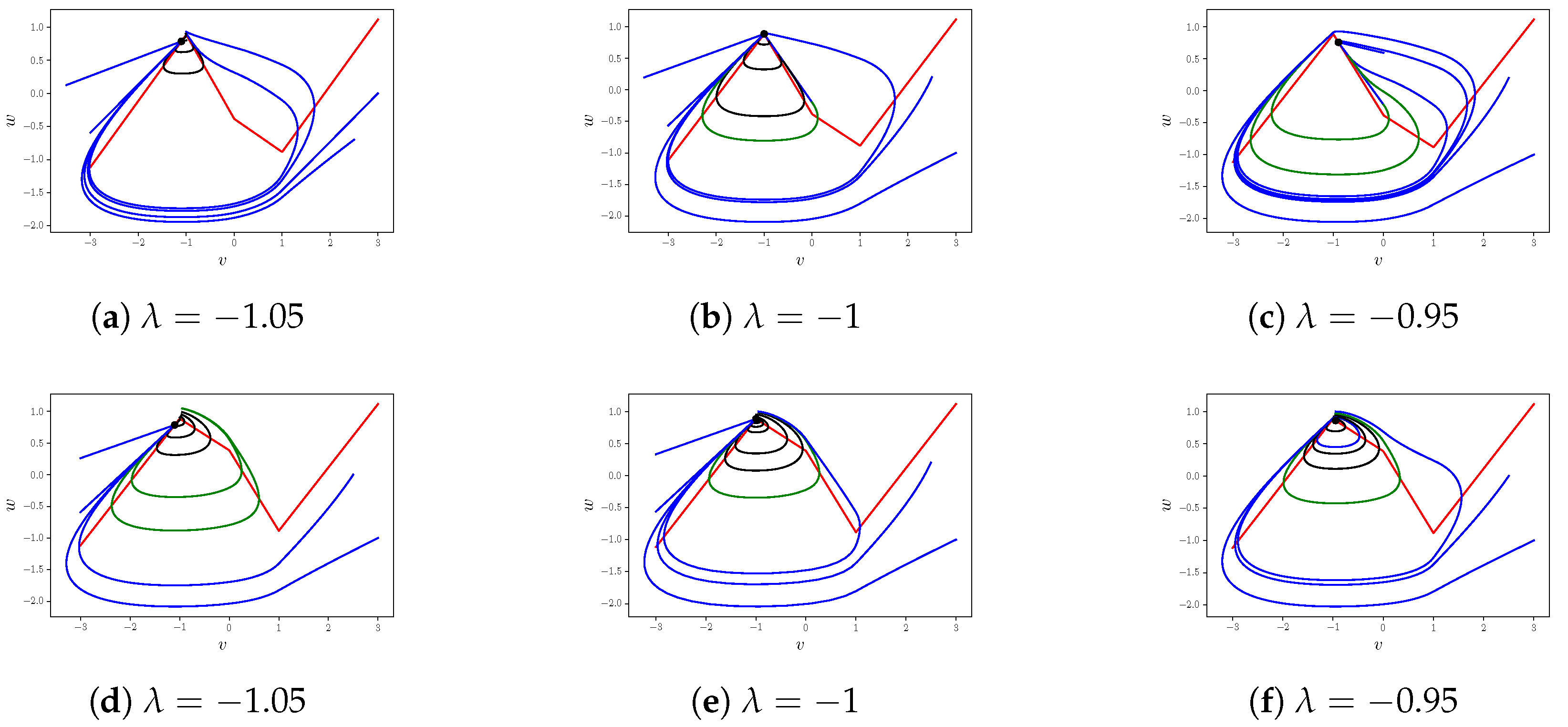
• Case $\lambda =-1$. The equilibrium $(-1,k)$ perpetually serves as the universal attractor for system (7), i.e., all trajectories tend towards the equilibrium as $t\to +\infty$. Although this equilibrium point is unstable, being either a node or a focus, when viewed from zone $R_1$, orbits that start with $v\left(0\right)>-1$ can diverge significantly from this equilibrium point, potentially traversing zones $R_1$, $R_2$, and even $R_{r,1}$. Regardless of this, because the orbits are ultimately bounded (as system (7) is dissipative) and no other equilibria exist, they will ultimately reach $v=-1$ at a point $(-1,w)$, where $w<k$. At this point, the stable node assumes dominance.
  In particular, for the node case, when ${\eta }_1^2-4ϵ\ge 0$, two linear invariant manifolds, which are unstable, extend from this equilibrium towards the right. The higher of these two invariant manifolds, which coincides for $-1\le v<v_1$ with the equation $w=({\eta }_1+\sqrt{{\eta }_1^2-4ϵ})(v+1)/2+k$, evolves into a maximal homoclinic orbit. However, in the focus case, when ${\eta }_1^2-4ϵ<0$, the system features a continuum of homoclinic orbits but lacks the maximal homoclinic orbit.
  Now, we show that system (7) undergoes a persistence bifurcation. According to Theorem 1, we have

  $${\mathit{N}}_{\mathbf{1}}=\left(\begin{array}{cc}-1& 1\\ -ϵ& 0\end{array}\right),{\mathit{N}}_{\mathbf{2}}=\left(\begin{array}{cc}-{\eta }_1& 1\\ -ϵ& 0\end{array}\right),{\mathit{C}}^{\mathit{T}}=\left(\begin{array}{cc}1& 0\end{array}\right),$$

  $${\mathit{E}}_{\mathbf{12}}=\left(\begin{array}{c}1-{\eta }_1\\ 0\end{array}\right),\mathrm{where}{\mathit{N}}_{\mathbf{2}}={\mathit{N}}_{\mathbf{1}}+{\mathit{E}}_{\mathbf{12}}{\mathit{C}}^{\mathit{T}},$$

  $$det\left({\mathit{N}}_{\mathbf{1}}\right)=det\left({\mathit{N}}_{\mathbf{2}}\right)=ϵ\ne 0,\mathrm{trace}\left({\mathit{N}}_{\mathbf{1}}\right)=-1,\mathrm{trace}\left({\mathit{N}}_{\mathbf{2}}\right)=-{\eta }_1,$$

  $$\mathrm{trace}\left({\mathit{N}}_{\mathbf{1}}\right)\mathrm{trace}\left({\mathit{N}}_{\mathbf{2}}\right)={\eta }_1<0,{\displaystyle \frac{1}{4}}=\mathrm{trace}{\left({\mathit{N}}_{\mathbf{1}}\right)}^2/4\ne det\left({\mathit{N}}_{\mathbf{1}}\right),$$

  $$ϵ=det({\mathit{N}}_{\mathbf{1}}+{\mathit{E}}_{\mathbf{12}}{\mathit{C}}^{\mathit{T}})\ne \mathrm{trace}{({\mathit{N}}_{\mathbf{1}}+{\mathit{E}}_{\mathbf{12}}{\mathit{C}}^{\mathit{T}})}^2/4={\displaystyle \frac{{\eta }_1^2}{4}},$$

  $${\mathit{N}}_{\mathbf{1}}^{-\mathbf{1}}={\displaystyle \frac{1}{ϵ}}\left(\begin{array}{cc}0& -1\\ ϵ& -1\end{array}\right).$$

  (22)
  Therefore, system (7) undergoes a persistence bifurcation at $\lambda =-1$ due to $1+{\mathit{C}}^{\mathit{T}}{\mathit{N}}_{\mathbf{1}}^{-\mathbf{1}}{\mathit{E}}_{\mathbf{12}}=1>0$; see Figure 2. Each phase portrait is generated using the Python software (Anaconda3-2020), with a specific value for the parameter $\lambda$ set for each simulation.
• Case $-1<\lambda <1$. The equilibrium is situated on either $L_1$ or $L_2$ and is characterized as either an unstable node or an unstable focus. In both cases, it is encircled by a unique stable limit cycle. In the focus scenario, the existence and uniqueness of this limit cycle are guaranteed by Theorem 1. Given that the system transitions from a focus to a node, the presence of a limit cycle is inevitable. Furthermore, since the node is stable, it follows that the associated limit cycle encircling an unstable focus must also be stable. Therefore, a supercritical Hopf bifurcation occurs as the parameter $\lambda$ crosses the value of $-1$.
  However, Theorem 1 does not apply to the node case. The existence and uniqueness of the limit cycle for the node case can be established through Theorem 1 from [31].
  It is important to recognize that the size of the limit cycle can change based on the nature of the equilibrium points within the system.

  1.

  Node case. In scenarios where the equilibrium is a node, there are two invariant manifolds present. The limit cycle lies outside these manifolds and cannot intersect with them. Since both linear segments, $L_1$ and $L_2$, act as repellers, the limit cycle must traverse through all four distinct regions of the phase space.

  2.

  Focus case. According to Theorem 1, when $\lambda =-1$, a limit cycle is present in regions $R_1$ and $R_{l,1}$. Conversely, when $\lambda =1$, a limit cycle is found in regions $R_2$ and $R_{r,1}$.

  The magnitude of the limit cycle can be summarized as follows.

  1.

  When ${\eta }_1^2-4ϵ\ge 0$, the limit cycle traverses across four distinct regions;

  2.

  When ${\eta }_1^2-4ϵ<0$, the limit cycle is confined to regions $R_1$ and $R_{l,1}$ as the parameter $\lambda$ is close to $-1$;

  3.

  When ${\eta }_2^2-4ϵ\ge 0$, the limit cycle passes through four distinct regions;

  4.

  When ${\eta }_2^2-4ϵ<0$, the limit cycle is restricted to regions $R_2$ and $R_{r,1}$ as $\lambda$ approaches 1.

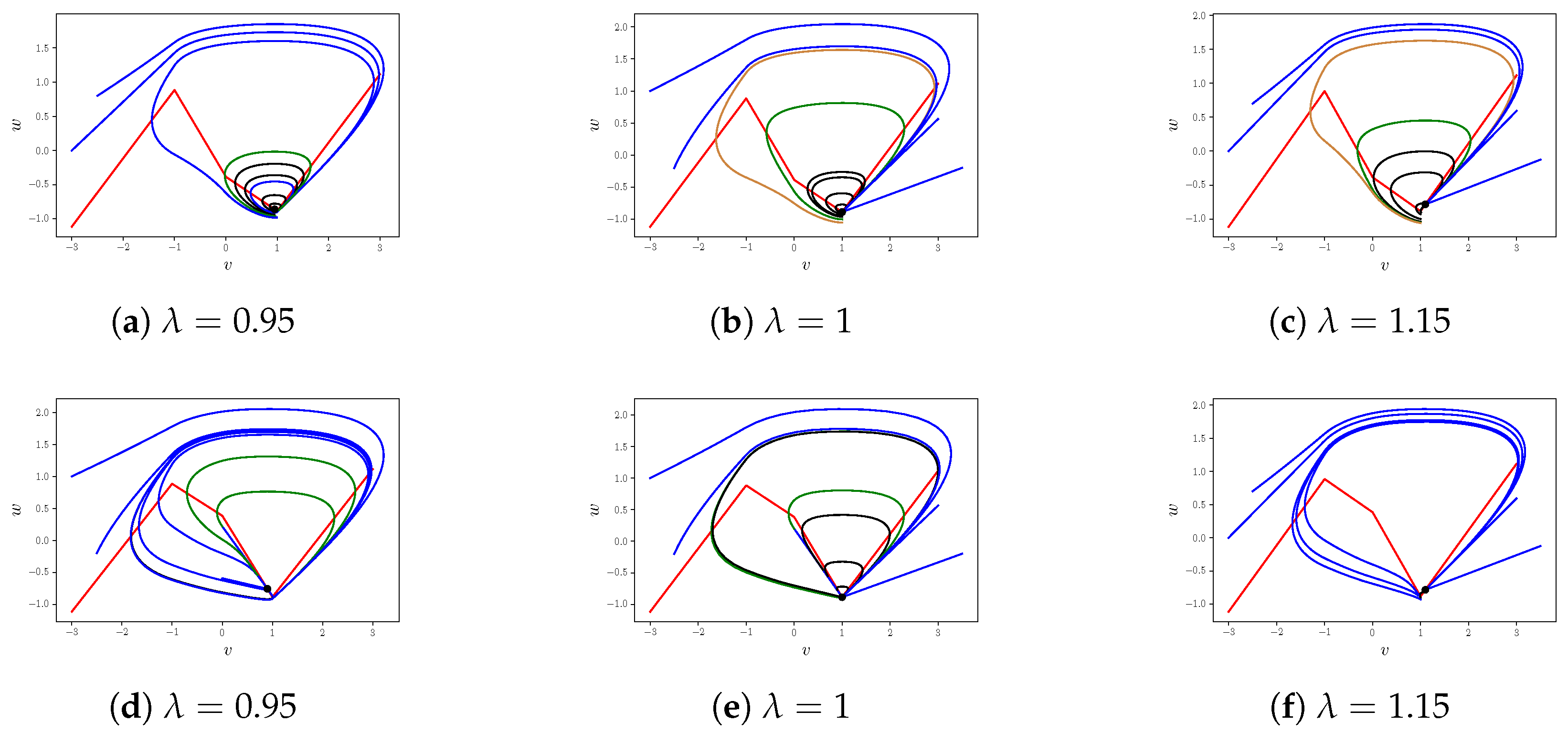
• Case $\lambda =1$. The equilibrium $(1,-k)$ is globally attractive. Although this equilibrium point is unstable, being either a node or a focus, when viewed from zone $R_2$, orbits that start with $v\left(0\right)<1$ can diverge significantly from this equilibrium point, utilizing zones $R_1$, $R_2$, and even $R_{l,1}$. Regardless of this, they will inevitably reach $v=1$ at $(1,w)$, where $w>-k$. At this point, the stable node takes over.
  Similarly to the case of $\lambda =-1$, for the node situation, the lower of two unstable invariant manifolds, which coincides for $v_1\le v<1$ with the equation $w=({\eta }_2+\sqrt{{\eta }_2^2-4ϵ})(v-1)/2-k$, evolves into a maximal homoclinic orbit. However, in the focus case, when ${\eta }_2^2-4ϵ<0$, the system possesses a continuum of homoclinic orbits but lacks the maximal homoclinic orbit.
  According to Theorem 1, we have

  $${\mathit{N}}_{\mathbf{3}}=\left(\begin{array}{cc}-{\eta }_2& 1\\ -ϵ& 0\end{array}\right),{\mathit{N}}_{\mathbf{4}}=\left(\begin{array}{cc}-1& 1\\ -ϵ& 0\end{array}\right),{\mathit{C}}^{\mathit{T}}=\left(\begin{array}{cc}1& 0\end{array}\right),$$

  $${\mathit{E}}_{\mathbf{34}}=\left(\begin{array}{c}{\eta }_2-1\\ 0\end{array}\right),\mathrm{where}{\mathit{N}}_{\mathbf{4}}={\mathit{N}}_{\mathbf{3}}+{\mathit{E}}_{\mathbf{34}}{\mathit{C}}^{\mathit{T}},$$

  $$det\left({\mathit{N}}_{\mathbf{3}}\right)=det\left({\mathit{N}}_{\mathbf{4}}\right)=ϵ\ne 0,\mathrm{trace}\left({\mathit{N}}_{\mathbf{3}}\right)=-{\eta }_2,\mathrm{trace}\left({\mathit{N}}_{\mathbf{4}}\right)=-1,$$

  $$\mathrm{trace}\left({\mathit{N}}_{\mathbf{3}}\right)\mathrm{trace}\left({\mathit{N}}_{\mathbf{4}}\right)={\eta }_2<0,\mathrm{trace}{\left({\mathit{N}}_{\mathbf{3}}\right)}^2/4={\displaystyle \frac{{\eta }_2^2}{4}}\ne det\left({\mathit{N}}_{\mathbf{3}}\right),$$

  $$ϵ=det({\mathit{N}}_{\mathbf{3}}+{\mathit{E}}_{\mathbf{34}}{\mathit{C}}^{\mathit{T}})\ne \mathrm{trace}{({\mathit{N}}_{\mathbf{3}}+{\mathit{E}}_{\mathbf{34}}{\mathit{C}}^{\mathit{T}})}^2/4={\displaystyle \frac{1}{4}},$$

  $${\mathit{N}}_{\mathbf{3}}^{-\mathbf{1}}={\displaystyle \frac{1}{ϵ}}\left(\begin{array}{cc}0& -1\\ ϵ& -{\eta }_2\end{array}\right).$$

  (23)
  Therefore, system (7) undergoes a persistence bifurcation at $\lambda =1$ due to $1+{\mathit{C}}^{\mathit{T}}{\mathit{N}}_{\mathbf{3}}^{-\mathbf{1}}{\mathit{E}}_{\mathbf{34}}=1>0$; see Figure 3.
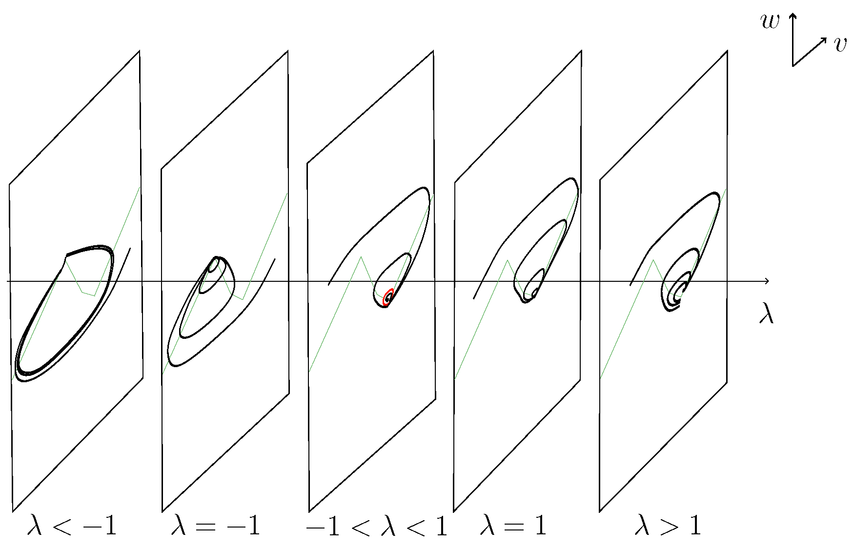
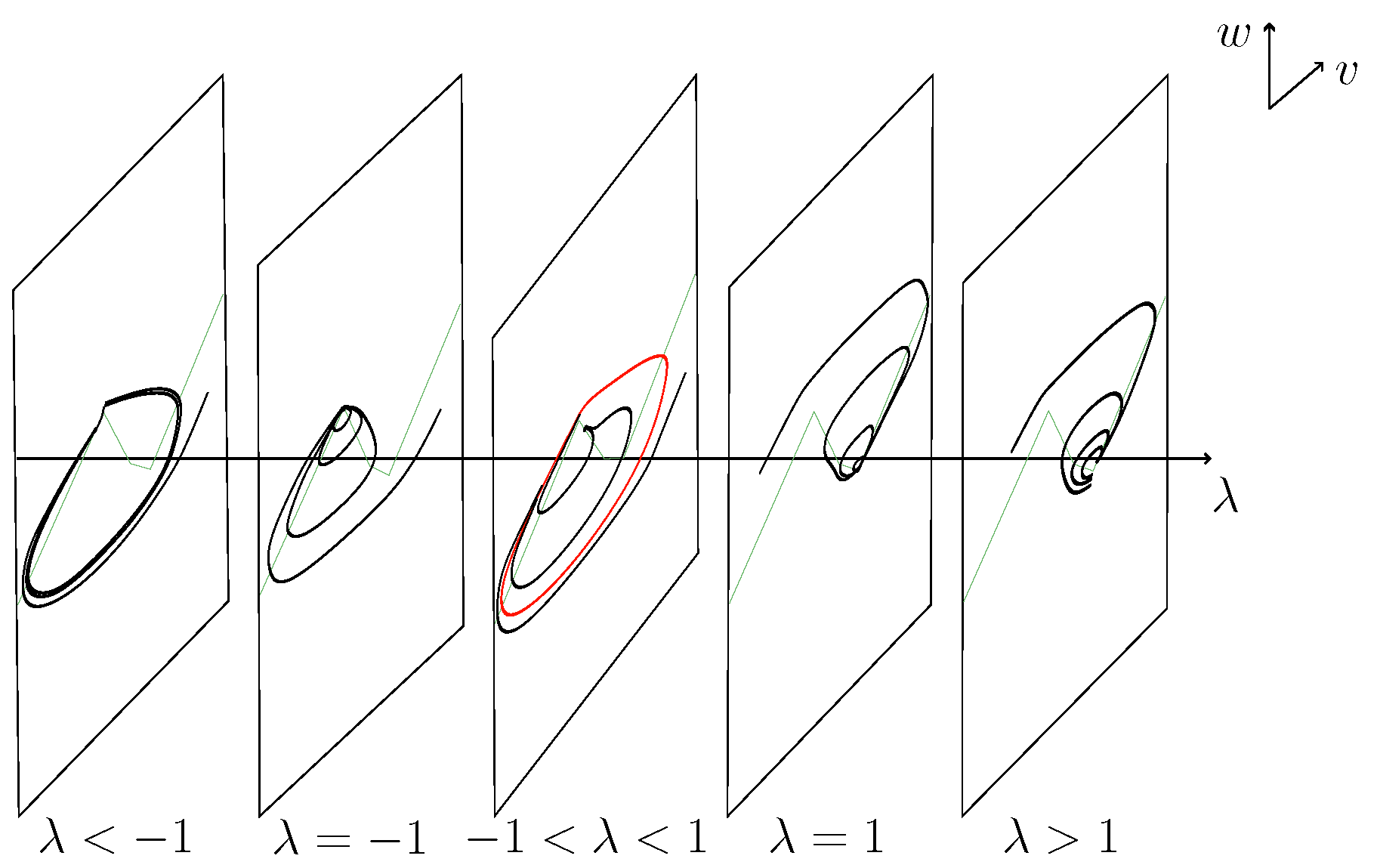
• Case $\lambda >1$. In this case, the unique equilibrium is located on $L_{r,1}$ and serves as the global attractor for system (7). A supercritical Hopf bifurcation takes place as $\lambda$ passes through the value of 1. Figure 4 and Figure 5 display schematic representations of the phase portraits that correspond to the full range of the parameter $\lambda$. These figures were created using Inkscape.

□

4. Comparison Between Models with Varying Quantities of Linear Segments

The piecewise linear system with three zones, as studied by Desroches et al. [17], is described as

$$\left\{\begin{array}{ccc}\hfill \dot{x}& =\hfill & y-f\left(x\right),\hfill \\ \hfill \dot{y}& =\hfill & ϵ(a-x).\hfill \end{array}\right.$$

(24)

where a is the bifurcation parameter, $k>0$ is a constant, and $f\left(x\right)$ is defined as

$$f\left(x\right)=\left\{\begin{array}{cc}x+k+1,\hfill & x<-1,\\ -kx,\hfill & -1\le x\le 1,\\ x-k-1,\hfill & x>1.\end{array}\right.$$

(25)

Here, a and $ϵ$ in system (24) correspond to $\lambda$ and $ϵ$ in our system (7), representing the bifurcation parameter and the time scale, respectively.

The comparison of the PWL VDP models with three or four segments can be summarized in terms of the following aspects.

1.

Parameters: In system (24), k represents both the ordinate of the highest point and the inverse of the slope of the middle linear segment, whereas in our system (7), k only represents the ordinate of the highest point. The slopes of the middle segments are denoted by ${\eta }_1$ and ${\eta }_2$ and related via (21).

2.

Dynamical behavior: Both models undergo a supercritical Hopf bifurcation and exhibit a continuum of homoclinic orbits at $\lambda =1$. In both systems, the presence of limit cycles is observed. This indicates that increasing the number of linear segments from three to four does not fundamentally alter the bifurcation structure of the system.

However, our system (7) allows for a more detailed analysis of the dynamics near $\lambda =-1$, revealing behavior analogous to that observed at $\lambda =1$. Moreover, from the perspective of a boundary equilibrium analysis, the persistence bifurcation at $\lambda =\pm 1$ has been investigated, which is not explicitly discussed in system (24). This provides additional insights into the system’s dynamics.

3.

Numerical simulations: Our numerical simulations (Figure 6) illustrate the phase portraits for both the three-zone and four-zone models. The simulations show that both models exhibit similar bifurcation structures and dynamical behaviors.

4.

Future work: Our study suggests that further research is necessary to explore the effects of increasing the number of linear segments beyond four. A generic conclusion on the impact of adding more linear segments on the system’s dynamics could provide deeper insights into the behavior of piecewise linear systems.

5. Conclusions and Future Work

In this work, we investigated the dynamics and bifurcations of a PWL VDP model that encompassed four distinct zones. Specifically, the critical manifold of this model was composed of four segments $L_{l,1}\cup L_1\cup L_2\cup L_{r,1}$. The results showed that a complicated bifurcation occured at $\lambda =-1$ and $\lambda =1$, which was the combination of a persistence bifurcation and the appearance of small- or large-amplitude limit cycles. Compared to the work in [17], we analyzed the bifurcation occurring at $\lambda =-1$ and introduced the boundary equilibrium bifurcation. Finally, we compared the two systems and found that the topology of the PWL VDP equation remained unaffected upon increasing the number of linear segments from three to four.

Another interesting task would be to devise a generic conclusion about the effect of increasing the number of linear segments on the system’s dynamics. Specifically, future work could explore whether adding more linear segments (i.e., beyond four) leads to significant changes in the system’s bifurcation structure or dynamical behavior. Additionally, it would be valuable to investigate the implications of these findings for real-world applications, particularly in engineering and neuroscience, where piecewise linear models are often used to simplify complicated nonlinear systems.

References

- van der Pol, B. Forced oscillations in a circuit with nonlinear resistance. Philos. Mag. 1927, 3, 65–80. [Google Scholar] [CrossRef]
- King, G.P.; Gaito, S.T. Bistable chaos. I. Unfolding the cusp. Phys. Rev. A 1992, 46, 3092–3099. [Google Scholar] [CrossRef] [PubMed]
- Matouk, A.E.; Agiza, H.N. Bifurcations, chaos and synchronization in ADVP circuit with parallel resistor. J. Math. Anal. Appl. 2008, 341, 259–269. [Google Scholar] [CrossRef]
- Zhao, H.; Lin, Y.; Dai, Y. Hidden attractors and dynamics of a general autonomous van der Pol–Duffing oscillator. Int. J. Bifurc. Chaos 2014, 24, 1450080. [Google Scholar] [CrossRef]
- Izhikevich, E.M. Neural excitability, spiking, and bursting. Int. J. Bifurc. Chaos 2000, 10, 1171–1266. [Google Scholar] [CrossRef]
- Glass, L.; Mackey, M.C. From Clocks to Chaos: The Rhythms of Life, 1st ed.; Princeton University Press: Princeton, NJ, USA, 1988. [Google Scholar]
- Lichtenberg, A.J.; Lieberman, M.A. Regular and Chaotic Dynamics, 2nd ed.; Springer: New York, NY, USA, 2013. [Google Scholar]
- Brock, W.A.; Hommes, C.H. A Rational Route to Randomness. Econometrica 1997, 65, 1059–1095. [Google Scholar] [CrossRef]
- Nayfeh, A.H.; Mook, D.T. Nonlinear Oscillations; WILEY-VCH: Weinheim, Germany, 2004. [Google Scholar]
- Alhejaili, W.; Salas, A.H.; El-Tantawy, S.A. Approximate solution to a generalized Van der Pol equation arising in plasma oscillations. AIP Adv. 2022, 12, 105104. [Google Scholar] [CrossRef]
- Leung, A.Y.T.; Yang, H.X.; Guo, Z.J. The residue harmonic balance for fractional order van der Pol like oscillators. J. Sound Vib. 2012, 331, 1115–1126. [Google Scholar] [CrossRef]
- Herişanu, N.; Marinca, V. An iteration procedure with application to Van der Pol oscillator. Int. J. Nonlinear Sci. Numer. Simul. 2009, 10, 353–361. [Google Scholar] [CrossRef]
- Kimiaeifar, A.; Saidi, A.R.; Bagheri, G.H.; Rahimpour, M.; Domairry, D.G. Analytical solution for Van der Pol-Duffing oscillators. Chaos Solitons Fractals 2009, 42, 2660–2666. [Google Scholar] [CrossRef]
- Ndam, J.N.; Adedire, O. Comparison of the solution of the Van der Pol equation using the modified Adomian decomposition method and truncated Taylor series method. J. Niger. Soc. Phys. Sci. 2020, 2, 106–114. [Google Scholar] [CrossRef]
- Huang, X.L.; Xu, J.; Wang, S.N. Nonlinear system identification with continuous piecewise linear neural network. Neurocomputing 2012, 77, 167–177. [Google Scholar] [CrossRef]
- Katagiri, T.; Saito, T.; Komuro, M. Lost solution and chaos. IEEE Int. Symp. Circuits Syst. 1993, 4, 2616–2619. [Google Scholar]
- Desroches, M.; Freire, E.; Hogan, S.J.; Ponce, E.; Thota, P. Canards in piecewise-linear systems: Explosions and super-explosions. Proc. R. Soc. A. 2013, 469, 20120603. [Google Scholar] [CrossRef]
- Rotstein, H.G.; Coombes, S.; Gheorghe, A.M. Canard-like explosion of limit cycles in two-dimensional piecewise-linear models of FitzHugh-Nagumo type. SIAM J. Appl. Dyn. Syst. 2012, 11, 135–180. [Google Scholar] [CrossRef]
- Arima, N.; Okazaki, H.; Nakano, H. A generation mechanism of canards in a piecewise linear system. IEICE Trans. Fundam. Electron. Commun. Comput. Sci. 1997, 80, 447–453. [Google Scholar]
- Carmona, V.; Fernández-García, S.; Teruel, A.E. Saddle-node canard cycles in slow-fast planar piecewise linear differential systems. Nonlinear Anal. Hybrid Syst. 2024, 52, 101472. [Google Scholar] [CrossRef]
- Chen, H.B.; Jia, M.; Tang, Y.L. Topological classifications of a piecewise linear Liénard system with three zones. J. Differ. Equ. 2024, 399, 1–47. [Google Scholar] [CrossRef]
- Fernández-García, S.; Desroches, M.; Krupa, M.; Teruel, A.E. Canard solutions in piecewise linear systems with three zones. Dyn. Syst. Int. J. 2016, 31, 173–197. [Google Scholar] [CrossRef]
- Li, S.; Llibre, J. Canard limit cycles for piecewise linear Liénard systems with three zones. Int. J. Bifurc. Chaos 2020, 30, 2050232. [Google Scholar] [CrossRef]
- Llibre, J.; Nuñez, E.; Teruel, A.E. Limit cycles for planar piecewise linear differential systems via first integrals. Qual. Theory Dyn. Syst. 2002, 3, 29–50. [Google Scholar] [CrossRef]
- Zegeling, A. Perturbation of a piecewise regular-singular Liénard system. J. Differ. Equ. 2024, 380, 404–442. [Google Scholar] [CrossRef]
- Roberts, A. Canard explosion and relaxation oscillation in planar, piecewise smooth, continuous systems. SIAM J. Appl. Dyn. Syst. 2016, 15, 609–624. [Google Scholar] [CrossRef]
- Roberts, A.; Gendining, P. Canard-like phenomena in piecewise-smooth Van der Pol systems. Choas 2014, 24, 023138. [Google Scholar] [CrossRef]
- Sekikawa, M.; Inaba, N.; Tsubouchi, T. Chaos via duck solution breakdown in a piecewise linear van der Pol oscillator driven by an extremely small periodic perturbation. Phys. D 2004, 194, 227–249. [Google Scholar] [CrossRef]
- di Bernardo, M.; Budd, C.J.; Champneys, A.R.; Kowalczyk, P. Piecewise-Smooth Dynamical Systems Theory and Applications, 1st ed.; Spring: Berlin/Heidelberg, Germany, 2008. [Google Scholar]
- Krylov, N.M.; Bogoliubov, N.N. Introduction to Non-Linear Mechanics, 1st ed.; Princeton University Press: Princeton, NJ, USA, 1950. [Google Scholar]
- Llibre, J.; Ordóñez, M.; Ponce, E. On the existence and uniqueness of limit cycles in planar continuous piecewise linear systems without symmetry. Nonlinear Anal.-Real 2013, 14, 2002–2012. [Google Scholar] [CrossRef]