Abstract
Superstring compactifications have been vigorously studied for over four decades, and have flourished, involving an active iterative feedback between physics and (complex) algebraic geometry. This led to an unprecedented wealth of constructions, virtually all of which are “purely” algebraic. Recent developments however indicate many more possibilities to be afforded by including certain generalizations that, at first glance at least, are not algebraic—yet fit remarkably well within an overall mirror-symmetric framework and are surprisingly amenable to standard computational analysis upon certain mild but systematic modifications.
MSC:
14D06; 14J32; 32Q25; 81T39; 83E30
1. Introduction, Rationale, and Summary
For over a century, classical geometry of spacetime has been identified with solutions to Einstein’s field equations, , given here in the “trace-reversed form”: is the Ricci tensor and the energy-momentum density tensor of matter present in the region of interest. The geometry of empty spacetime () is, thus, by definition Ricci-flat. This general qualification is remarkably persistent, through higher-dimensional models and including string theory, where it insures quantum stability to lowest order in string tension [1,2,3,4], and then also emerges in the full, oriented loop-space reformulation [5,6,7,8,9,10,11,12,13,14,15]. Modulo additive total derivatives, is the first Chern class of the underlying spacetime, which links to topology and algebraic geometry and identifies stringy spacetimes, , by the hallmark “Calabi–Yau” condition, [15].
Models within this string theory framework that come close to reproducing the observed world include “Calabi–Yau compactifications” [15,16] and their various generalizations, described by additional conditions involving higher Chern classes of and of a variety of additional structures, typically defined over . For example, the “Hull–Strominger system” [17,18,19,20,21] allows (geometric) torsion in and with additional gauge-field fluxes (possibly deforming its tangent bundle to higher-rank stable bundles) leads to more general, non-Kähler compactifications [22,23] (The underlying worldsheet formulation of string theory pairs its ubiquitous antisymmetric abelian gauge 2-form with the metric into the complex combination, , at least if the target spacetime (or a factor thereof) permits a locally defined complex structure. The so-complexified metric structure on the target space a priori permits the metric itself to degenerate at certain locations if balanced by a non-degenerate there. This is the general mechanism that extends (analytically continues) GLSMs from a (familiar) “geometric” target space to various other “non-geometric” descriptions [24,25]; subsequent analyses have then described those phases using some different geometry, such as stratified pseudo-manifolds turning up in [26] and discussed further in [27], and perhaps even more general notions of geometry may be implied by the inclusion of more general “defects” [28,29]). A survey of considered spacetime geometries aiming also for the observed 3+1-dimensional asymptotically de Sitter spacetime, as given in [30], indicates some of the complexities of our ultimate goal.
Since the pioneering works of Refs. [31,32], all algebraic constructions start from some well-understood ambient (embedding) space, X, within which the desired geometries are found as solutions of systems of algebraic equations, . To this end, X is typically chosen to have some degree of (quasi) homogeneity [15], which corresponds to a gauge symmetry in the underlying super-conformal quantum field theory on the worldsheet swept by the superstring. With at least -supersymmetry and abelian gauge symmetry on the worldsheet, this defines the broad class of gauged linear sigma models (GLSMs) [24,25,33,34] and billions of catalogued Calabi–Yau 3-folds [35,36,37,38,39,40,41,42,43]. Many of the half a billion convex reflexive polytopes [42,43] admit distinct triangulations, leading to distinct toric varieties, and so, to distinct deformation families of hypersurfaces in them. Each of these constructions admits additional variations by deforming the tangent bundle of the hypersurface and extending it via additional line-bundles, ultimately leading to an astounding combinatorial wealth [44]. These constructions are vigorously studied by physicists (mostly string theorists) and mathematicians (mostly algebraic geometers) alike, owing to the inherent use of complex algebraic and toric geometry [45,46,47,48,49].
The impressive body of work related to these complex algebraic toric geometry constructions notwithstanding, the original string theory requirements mentioned in the second paragraph in fact mandate neither supersymmetry nor complex structure in the “target spacetime”, . Indeed, neither of these structures is guaranteed in the requisite worldsheet -supersymmetric formulation; see [50,51,52,53] and much more recently [54] for another foundational aspect. In this sense, target spacetime supersymmetry and complex structure (at least in the compact factors of ) provide a robust and rigid framework affording a very high degree of computability, a vast array of lampposts to illuminate the landscape (This reminds of Danilov’s description of “frigid toric crystals” [46], §0.6, p. 100). However, such models can at most be regarded as an approximation to describing the real world, where supersymmetry is at most a broken symmetry. It is then very gratifying to find that the transposition mirror model construction [55,56,57,58] does extend to the more general spaces described in Refs. [59,60,61,62,63]—although many of the details (and possible limitations!) of such extensions still remain to be determined, especially from the symplectic geometry vantage point.
The primary objective of this article, then, is to serve as a descriptive and motivational rallying exposition of these extensions, calling attention both to their established features and to some of the key open questions. This aims to catalyze further research towards a more robust (foundational, rigorous) and comprehensive understanding. To that end, Section 2 presents and explores an infinite sequence of GLSMs, the ground states of which form double deformation families of Calabi–Yau hypersurfaces in Hirzebruch scrolls; their analysis is facilitated by being realized both in the (complex-algebraic) toric geometry framework and as generalized complete intersections in products of projective spaces. Section 3 presents how the transposition mirror construction extends to these models and provides for a vast combinatorial array of multiple mirrors. Section 4 concludes by highlighting some open questions and concerns brought about by extending the construction and computational framework to include embedding Calabi–Yau manifolds in non-Fano algebraic varieties as well as non-algebraic torus manifolds, which will hopefully serve as a challenge for future development.
2. A Showcasing Deformation Family
Expanding on earlier work [59,60,61,62], I focus on a particular infinite sequence of constructions corresponding to Calabi–Yau hypersurfaces in Hirzebruch scrolls, the rich mathematical history of the latter [45,47,48,49,64] affording their study from multiple different points of view, including their realization within GLSM models [25]—which is where we start.
2.1. From GLSM to Toric
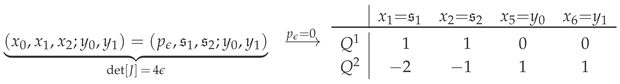
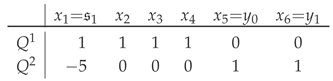
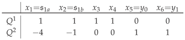
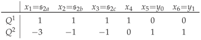
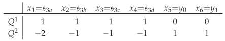
Let us begin with listing a collection of (chiral superfield) variables and their -charges:
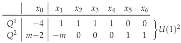 The fact that cancels (for each ) the sum of charges of the other variables guarantees that the gauge anomalies cancel, and also that the product is -invariant, and so, admissible in the superpotential. may be thought of as a quantum field theory generalization of a Lagrange multiplier [24,53,65,66,67]. Owing to its ubiquitous importance in the algebraic geometry of the deformations of the superpotential, has been dubbed the “fundamental monomial” [68]; see also [69].
The choice of the superpotential provides part of the defining equations for the “ground state variety”, by definition of the potential energy:
where is the general form of the superpotential, , and is the (twisted-chiral superfield) variable corresponding to the gauge group [24,25]. Supersymmetric ground states are zeros of (2), and the combined vanishing of the first (“F”) and second (“D”) terms in (2) associate distinct -regions with the distinct -orbits in the -space. In particular, provides the “geometric phase”, wherein the location:
is excluded; for details of the GLSM motivations and the other phases/options, see [24,25,60]. The remaining X-space is projectivized by the supersymmetry-complexified gauge symmetry, , specifying the Hirzebruch scroll, . Indeed, in (1) will be identified with its Cox coordinates, and the -rows specify its Mori vectors and Chern class [49],
so also guarantees the zero-locus, , to be Ricci-flat.
2.1.1. The Superpotential
The general form of implies at the minimum of (2):
This is highly singular for the simple choice , which we aim to smooth by including other charge- monomials, which are of the form:
This at once shows that for , the monomials (6) are either all proportional to or involve negative powers of . Standard practice in both quantum field theory and algebraic geometry is to omit rational monomials, which crucially hobbles the intended deformations: restricting to insures that all regular polynomial choices,
necessarily factorize so that the zero-locus reduces: , and the singular locus, is a Calabi–Yau 2-fold. The 3-fold is Tyurin degenerate [61] and deemed “unsmoothable”, as there are no regular monomials to render (7) transverse.
In turn, setting in (6) identifies monomials that are -independent, and so, can smooth (7) by deforming it away from .
To this end, compare the -degree monomials for and , shown in Figure 1 for the two-dimensional surfaces (adjusting to and omitting ) for simplicity.
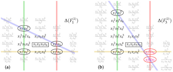
Figure 1.
Some of the -degree monomials plotted to indicate (by colored lines) the “stripes” discussed in the text; the fundamental monomial, is boxed. The left-hand side diagram (a) displays anticanonical monomials for , while the right-hand side diagram (b) shows those for .
The plots in Figure 1 make evident that:
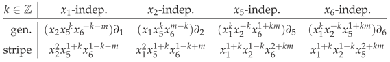
- Monomials independent of a particular variable occur along a straight-line “stripe” (hyperplane in higher dimensions). Therefore, each “stripe” is a suitable multiple of a single -derivative, :
 Since , each “stripe” acts as a boundary for that -deformation.
 - “Cornerstone” monomials at the intersection of two “stripes” are independent of two variables; this hierarchy extends straightforwardly in higher dimensions. The tabulation (8) makes it clear that: (1) There is no - and -independent monomial. (2) There is an - and -independent monomial only for , and , respectively. (3) The “cornerstone” monomials are , , , and , and are circled in the plots in Figure 1.
- The above shows that deforming the fundamental monomial equips the system of anticanonical monomials with the hierarchical structure of a poset:
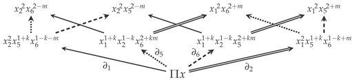
Being reachable by a simple (first) derivative from the fundamental monomial, , monomials on each -independent “stripe” are at a (deformation) distance of 1 from , with the direction of the respective deformations indicated by the Euclidean lattice normals:
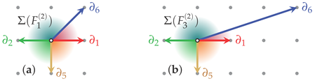 Each two-dimensional cone enclosed between two of these consecutive directions corresponds to a (circled) corner monomial in Figure 1: , , etc. The so-constructed fan of cones, , in fact specifies the Hirzebruch scroll as a toric variety [47,48,49].
The fans (10) have a natural dimension-ranked poset structure generated by the inclusion of cones in the boundary of one-higher dimensional cones, and isomorphic to (9). In (10), the central 0-cone is within the boundary of the 1-cone , which is within the boundary of the 2-cone . This chain of relations is strictly (inclusion-reversing) dual to the corresponding statements regarding the monomials in Figure 1; for example:
Also of note is the fact that the two-dimensional cones and do not belong to either of the two (posets) fans (10); this defines the so-called Stanley–Reisner ideal among the linear vector (sub)spaces generated by [49]. Dually in Figure 1, the two vertical “stripes” (monomials without and without , respectively) never intersect, and the horizontal (-omitting) “stripe” intersects the slanted (-omitting) “stripe”, either outside the distance-1 convex polygon enclosing the universal monomial, , or at a non-lattice location, for , where that distance-1 enclosing polygon self-intersects; this defines the so-called “irrelevant” ideal among the multiplicative ring of monomials [49].
2.1.2. The Transpolar Operation
The “stripe”-wise dual operation used above to map the monomial systems in Figure 1 to the fans (10) is a simple version of the transpolar operation (denoted by “▿”; see Section 3) defined more formally in Refs. [60,61,62]. It implements the standard polar operation of algebraic toric geometry [47,48,49] for each (convex subset of each) face of a polytope, then reassembles the resulting elements using the canonical inclusion-reversing nature of any duality. Moreover, the same iterative operation also works perfectly in reverse: The Euclidean normal to the “stripe” in (10) is and indicates for and for ; the normal to in (10, a) is and indicates for , while the normal to in (10, b) is and indicates for , and so on. The key distinction in between (convex and flat) and (self-intersecting, i.e., flip-folded) cases reflects the fact that the integral hull (lattice enclosure) of is convex for but non-convex for .
This transpolar operation is markedly unlike the standard polar operation. (It was highly amusing to learn that many active researchers in algebraic toric geometry, while always citing the standard (global) polar operation, in practice often use variants of the (local) “stripe”-wise dual (dubbed “transpolar” [60]) operation—the original invention of which is “lost in the mists of time”; I thank Hal Schenck for communicating these tidbits.) Defined globally over the entire polyhedral body at once, when starting from in (10), the standard polar operation automatically replaces it with the convex hull, which obscures the generator ; the so-chosen monomial set in Figure 1b stops at the intersection of the slanted and horizontal “stripes”, never reaching the right-hand side vertical (red) stripe of monomials (which are indeed all rational). When starting from in Figure 1b, including also the right-hand side circled monomials, the standard polar maps only to . When omitting the right-hand side circled monomials, the right-most remaining monomials include and define a distance-0 “stripe”, which cannot define a Euclidean normal: Not only is the standard polar operation not involutive, but it is ill-defined for when —which are non-Fano.
Comparing the two monomial plots in Figure 1 and their transpolar images in (10) reveals several key features. Whereas the simple, flat fans in (10) evidently subdivide the (enveloping) polygons that span them, the arrangements of “stripes” present a non-trivial distinction: The left-hand side is a plain, flat trapezoid and has a simple subdividing fan. In turn, is subdivided by a fan-like structure (corresponding to a toric space) if it is understood to be a flip-folded and multilayered multitope, which spans and is subdivided by a multifan [70,71,72,73,74,75,76,77]; see also [78,79,80,81]. We will return to this in Section 3.
Corollary 1.
For a list of (chiral superfield) variables and their -charges as in (1), the most general superpotential, W in (2), is an -multiple of a deformation the fundamental monomial, . The lattice of all candidate monomials, , has hyperplanes at 1-derivative distance from , the deformation directions of which span the (multi) fan, , that corresponds to the underlying toric (ambient) space wherein the ground states minimize the potential (2).
The so-defined mapping a priori and by definition selects the transpolar extension [60,61,62] of the standard polar operation [47,48,49].
Remark 1.
Curbing the -deformations (as in Figure 1) to only the regular monomials (with only non-negative powers) in the selected (Cox) variables (1) restricts the transpolar mapping so it agrees with the standard polar operation—but only provided “fractional”, non-lattice locations are also included: In in Figure 1, this is the intersection of the slanted and horizontal “stripes”, which corresponds to . This is also beyond the standard practice in complex-algebraic toric geometry (The radical monomial, , reminds us of similar factors that were found to play the role of “twisted vacua” in Landau–Ginzburg orbifolds [82]. The self-crossing region in the complete Newton multitope, , for corresponds to monomials of the form , which depend only on the fiber coordinates in , but where the first, radical factor has degree of the volume-from of the base-. This is indeed the “hallmark” quality whereby radical monomials enable representing “non-polynomial” deformations [82]. For , such radical deformations are still proportional to a positive power of , and so, could not smooth the Tyurin-degenerate regular Calabi–Yau hypersurfaces.) The oft-required “regularity” (non-negative powers) depends on the choice of variables, and is not as unequivocal as may be expected; see (13) and (14) below.
Remark 2.
The foregoing extends to systems of multiple defining constraints: complete intersections, certain non-complete intersections, and higher-rank constraints defined by exact sequences of direct sums of line-bundles are straightforward (though tedious) [15]. Extensions to non-abelian GLSM gauge groups, while also possible [83,84], are beyond our present scope.
Remark 3.
Regarding the system of anticanonical monomials (as in Figure 1) as candidate -directional (10) deformations of the fundamental monomial, , shows that the distance-1 rational monomial deformations are all, a priori, “accessible”—by deforming in only one -direction at a time. In Figure 1b plot, the distance-1 monomials in the right-hand side vertical (red) “stripe” form the boundary for -deformations. Among them, is indeed inaccessible by -deformations and by -deformations; they are accessible as - and -multiples of -deformations, wherein do not vary. The standard polar operation [47,48,49] imposes such limitations all at once and is in this sense “global”. In contradistinction, the “stripe”-wise transpolar operation [60,61] is “local”.
Remark 4.
Conversely, the principal reason for including the rational sections such as and in Figure 1b is that the segment of “stripe” they form is transpolar to the -deformation, which is a generator of the fan (10, b) that encodes ; see also Figure 4, below. Omitting the -generator from (10, b) and its transpolar (rational) monomials encodes .
2.2. From Toric to Generalized Intersections
While ultimately interested in Calabi–Yau hypersurfaces in 4-folds, we note that the two particular Hirzebruch scrolls defined by the fans (10) and equipped with the anticanonical sections plotted in Figure 1 are well known to be diffeomorphic to each other; they are the same real, smooth manifold equipped, however, with discretely distinct complex structures. Nevertheless, there exists an explicit, continuous -deformation family of hypersurfaces, extending Hirzebruch’s original [64]:
At the center, , is Hirzebruch’s original scroll, , herein denoted ; extending defines as the zero-locus of the same . Hirzebruch scrolls have a hallmark submanifold, the directrix [45] with a maximally negative self-intersection (), and which can actually be specified as an explicit hypersurface even in the realization (12), using a recent construction [85]; see also [59,61,86] for an explicit algorithm. The degree of the directrix (with respect to ) must be , which of course cannot be holomorphic on all of . However, the equivalence class
is indeed holomorphic on : Each of the two representatives is manifestly holomorphic over their respective (one-point-punctured) part of , and their difference on the overlap is a finite multiple of , which vanishes on by definition. Furthermore, the constant-Jacobian variable change
 is a coordinate-level identification of this hypersurface with the toric rendition of , and where the components of the row-wise) Mori vectors are equal to the homogeneity degrees.
Away from the center, when , the directrix-defining Section (13) fails to be holomorphic, but is replaced by two that are holomorphic:
The constant-Jacobian change of variables
 maps this -family of hypersurfaces to a “cousin” of Hirzebruch’s scroll, which one might denote . In the GLSM, the charges (17) are trivially redefined:
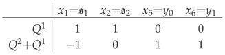 specifying the Mori vectors of the standard —consistent with the well-known diffeomorphism , for . It is tempting to conjecture [63] that the Segré-like change of variables
provides for the diffeomorphism: Its Jacobian () is non-constant and vanishes (the inverse diverges) over the poles of , where it can be modified by partitions of unity (“bump functions”) to make (19) a smooth but non-biholomorphic diffeomorphism. Although the foregoing discussion for simplicity focuses on simple two-dimensional showcasing examples, generalizations to higher dimensions are straightforward, as a few examples below will show.
specifying the Mori vectors of the standard —consistent with the well-known diffeomorphism , for . It is tempting to conjecture [63] that the Segré-like change of variables
provides for the diffeomorphism: Its Jacobian () is non-constant and vanishes (the inverse diverges) over the poles of , where it can be modified by partitions of unity (“bump functions”) to make (19) a smooth but non-biholomorphic diffeomorphism. Although the foregoing discussion for simplicity focuses on simple two-dimensional showcasing examples, generalizations to higher dimensions are straightforward, as a few examples below will show.
Remark 5.
The evidently self-consistent and effective use in the above context of sections that are equivalence classes of Laurent polynomials in terms of homogeneous coordinates, but regular (Cox) variables in the toric reformulation, lends support to the concerns about the choice of variables raised in Remark 1. One may wonder if a better choice of variables might render the Laurent (rational-monomial) deformations, such as those encircled in the right-hand side vertical “stripe” of the plot in Figure 1b; this is revisited in Section 4.
2.3. The Deformation Family Picture
Following the example in Section 2.2, consider now the explicit three-dimensional double deformation family of Calabi–Yau hypersurfaces in Hirzebruch scrolls, themselves defined as hypersurfaces in :
The so-constructed smooth Calabi–Yau manifolds have and , so and . Introduced and dubbed “generalized complete intersections” [85], in such deformation families, the second constraint polynomial, , is defined as a holomorphic section only on the zero locus of the first, and their choices are correlated. This structure also has a well-defined scheme-theoretic formulation over [86] and is amenable to a minor modification of the standard (co)homological algebra computations [59]. Here, we focus on the -family of first hypersurfaces,
which consist of various four-dimensional Hirzebruch scrolls [61,63]. Within these, we then find correlated, , Calabi–Yau three-dimensional hypersurfaces, the defining sections of which are closely related to the directrices (13) and (15)–e:dx2+1b.
- :
At the center, the hypersurface has the single, degree- directrix,
By the constant-Jacobian variable change à la (14), this identifies :
 and also defines the correlated family of degree- sections:
where provide cubics that parametrize the deformation family of Calabi–Yau 3-folds in . As evident from the explicit factorization of (24), all such Calabi–Yau 3-folds are Tyurin degenerate, deemed unsmoothable (by regular anticanonical sections), but smoothed by the , rational sections (6), . They correspond to the segment of the right-hand side vertical distance-1 “stripe” in Figure 1b delimited by its intersections with the horizontal and the slanted “stripes” [60,61]. Tyurin degeneration is characterized by the singular set
which is a K3 surface, a Calabi–Yau matryoshka within the degenerate Calabi–Yau 3-fold .
and also defines the correlated family of degree- sections:
where provide cubics that parametrize the deformation family of Calabi–Yau 3-folds in . As evident from the explicit factorization of (24), all such Calabi–Yau 3-folds are Tyurin degenerate, deemed unsmoothable (by regular anticanonical sections), but smoothed by the , rational sections (6), . They correspond to the segment of the right-hand side vertical distance-1 “stripe” in Figure 1b delimited by its intersections with the horizontal and the slanted “stripes” [60,61]. Tyurin degeneration is characterized by the singular set
which is a K3 surface, a Calabi–Yau matryoshka within the degenerate Calabi–Yau 3-fold .
- :
The system is now deformed to:
By the constant-Jacobian variable change à la (17), this identifies :
 and also defines the correlated family of degree- sections:
where, again, provide cubics that parametrize the deformation family of Calabi–Yau 3-folds in this “cousin” Hirzebruch scroll, . Since (30) does not factorize, this already deforms from the Tyurin degeneration in (24). Indeed, generic choices of are expected to be singular at most at isolated points: is singular at nine points, .
and also defines the correlated family of degree- sections:
where, again, provide cubics that parametrize the deformation family of Calabi–Yau 3-folds in this “cousin” Hirzebruch scroll, . Since (30) does not factorize, this already deforms from the Tyurin degeneration in (24). Indeed, generic choices of are expected to be singular at most at isolated points: is singular at nine points, .
- :
The system is now deformed to:
By the constant-Jacobian variable change à la (17), this identifies :
 and also defines the correlated family of degree- sections:
where, again, provide cubics that parametrize the deformation family of Calabi–Yau 3-folds in this “cousin” Hirzebruch scroll, . Owing to the swapped sign of the -term, and are independent from each other and are also independent from .
and also defines the correlated family of degree- sections:
where, again, provide cubics that parametrize the deformation family of Calabi–Yau 3-folds in this “cousin” Hirzebruch scroll, . Owing to the swapped sign of the -term, and are independent from each other and are also independent from .
- :
The system is now deformed to:
By the constant-Jacobian variable change à la (17), this identifies :
 and also defines the correlated family of degree- sections:
where, again, now provide cubics that overabundantly parametrize the deformation family of Calabi–Yau 3-folds in this “cousin” Hirzebruch scroll, . Notice that owing to the swapped signs of the - and -terms, , and are independent sections.
and also defines the correlated family of degree- sections:
where, again, now provide cubics that overabundantly parametrize the deformation family of Calabi–Yau 3-folds in this “cousin” Hirzebruch scroll, . Notice that owing to the swapped signs of the - and -terms, , and are independent sections.
2.4. The Deformation Family Picture, in Depth
Changing variables as in (14) and (17), the directrices are identified as Cox coordinates in the toric realization of the sequence of Hirzebruch scrolls: (22) in , (27) and (28) in , (32)–(34) in , and (38)–(41) in . Here found as smooth hypersurfaces in along the explicit deformation path, , they are diffeomorphic by deformation, and provide a textbook example of “the same real manifold” with a complex structure that varies [87]—herein, discretely. Within each of these, there is an effectively 86-dimensional family of Calabi–Yau hypersurfaces, parametrized by the -cubics indicated in (24), (30), (36), and (43), among which only those in must be Tyurin degenerate; the other ones (moving leftward in the indicated explicit deformation path) acquire an increasing degree of variation and inevitably become transverse.
The real manifold underlying , , and of the “first” deformation family, , is also diffeomorphic to [88]. Indeed, the Segré-like mapping
converts
and so maps . This of course is not a biholomorphism, as the Jacobian of the mapping (44) is non-constant: vanishes (and the inverse diverges) over the poles of . This can be smoothed without changing the topology by means of local “bump-functions”, thereby realizing the non-holomorphic diffeomorphism . The so-encountered variants of the Hirzebruch scrolls have their hallmark holomorphic and so irreducible directrices of maximally negative self-intersection:
While identical as real, smooth manifolds, the maximally negative self-intersection numbers (46)–(49) distinguish the as complex manifolds. The degree- directrices, (28), (33), (34), and (39)–(41), have standard, positive self-intersections equal to . The last of the above-calculated, (49), is in fact identical to the self-intersection of the hallmark holomorphic and so irreducible directrix of ,
which supports the claim that even as complex manifolds, . Since is Fano, all its generic Calabi–Yau hypersurfaces are smooth.
2.5. The Deformation Family Picture, Layered
Consider now the -path within the double deformation family of generalized complete intersections (20):
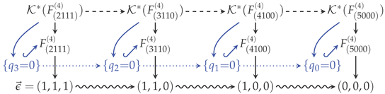
The deformation path in the -space (bottom row, wavy arrows) carries along:
- The sequence of (discrete) deformations among the Hirzebruch scrolls, (middle row in (51), no arrows drawn to avoid clutter), as discussed above.
- The sequence of (likewise discrete) deformations (top row in (51), dashed arrows) among the indicated anticanonical bundles, . This induces corresponding deformations on the anticanonical sections, which provide candidates for the sequence described next.
- The sequence of discrete “leafs” in the double deformations of the defining Equations (lower middle row in (51), dotted arrows) among the indicated Calabi–Yau hypersurfaces: the -dependent anticanonical bundles provide sections for the “second” deformation of anticanonical hypersurfaces, .
The diagram (51) prominently features the correlated triple consisting of:
- A well-understood embedding (“ambient”) space, X, chosen in (51).
- The anticanonical bundle, , and a collection of its sections, .
- The Calabi–Yau hypersurface—the zero locus, , of a selected anticanonical section.
Remark 6.
This entire triple plays a prominent role in the definition and analysis of GLSMs [24,25] and motivates in part the original proposal of Laurent deformations [60]. It is worth noting that is also a Calabi–Yau space, albeit non-compact. Also, between the non-compact -dimensional Calabi–Yau space, , and the compact -dimensional Calabi–Yau zero locus, , of a section of is the embedding space X, which is not Calabi—Yau, but wherein is an n-dimensional non-compact Calabi–Yau space [89,90]. This last fact seems to have been noticed only recently, and has so far not been explored.
2.6. Black Sheep in the Deformation Family
Exploring the diagram (51) now in the horizontal direction and knowing that all variants of the embedding space, , are in fact the same smooth real manifold, it is vexing to find that all anticanonical sections (24) on the far right of the diagram (51) factorize (see (7) for the GLSM/toric rendition), so that their zero loci, , are Tyurin degenerate Calabi–Yau varieties. They are deemed unsmoothable—since the deformations of are routinely limited to regular monomials (with non-negative powers) in the original variables (1). Indeed, omitted in (7) for are the monomials (6), which provide:
and are analogous to the monomials on the segment of the right-hand side vertical distance-1 “stripe” in Figure 1b delimited by its intersections with the horizontal and the slanted “stripe” [60,61]. Being independent of , the deformation (52) moves the zero locus away from the singularity . In the simpler notation of Section 2.1, direct computation then verifies that the generic combinations of (6) and (52) are transverse. For a simple example as in Section 2.2, consider the Calabi–Yau hypersurface in the family , defined as the zero locus of
Direct computation verifies that only when , which cannot happen in : The change of variables (14) implies that together with is equivalent to requiring , which does not exist in . With the restrictions (53), the cannot be absorbed into by their rescaling; the may be thought of as parametrizing a small deformation.
Having introduced rational-monomial deformations, the putative pole-locus must be addressed, to which end Ref. [60] employed the L’Hopital-like “intrinsic limit”:
Definition 1
Remark 7.
The pole-locus in (53) is , and the constraining condition (54) of Definition 1 is clearly well defined except along the zero locus of its denominator. That, however, intersects only at , where L’Hopital’s rule again gives (54) a well-defined value (zero). In general, such as when the requisite Laurent deformation has putative pole locations of higher order, the “intrinsic limit” will require additional iterations of applying L’Hopital’s rule. Although the pole locations will have a growing complexity and order in higher dimensions and higher “twist” (m) in , it would seem that the “intrinsic limit” resolution of the ambiguity in defining the zero locus, , i.e., specifying its closure is a well-defined procedure with a guaranteed finite completion. However, I am not aware of a proof.
Constrained (conditional) limits are far from novel in physics in general, making the “intrinsic limit” of [60] the “obvious” physics-motivated resolution of the ambiguity in defining the zero locus ; we return to this in Section 4. However, the use of the (constrained) limiting procedure definition of the so-defined (closure of the) zero locus clearly veers outside the usual framework of algebraic geometry.
Conjecture 1.
Laurent-deformed Calabi–Yau hypersurfaces closed/completed by the “intrinsic limit” (Definition 1) are not algebraic varieties; they are toric spaces, equipped with a maximal -action, and corresponding - or even fully -equivariant (co)homology.
Having veered outside the standard framework of complex algebraic (toric) geometry in trying to smooth the “unsmoothable” Tyurin-degenerate models opens a whole host of questions. For example, consider the preimage of ; under the sequence of deformations, all the way in the left-hand side of the diagram (51), where it has many (complex-algebraic, regular-monomial) smoothing deformations. Since can be smoothed by Laurent (rational-monomial) deformations, it is not unreasonable to propose:
3. Transposition Mirrors
The inclusion of spaces of which the construction veers outside of the routine complex-algebraic (toric) geometry to include spaces that are not algebraic (such as the “intrinsic limit”-completed/closed zero loci of Laurent defining polynomials) has rather novel consequences via mirror symmetry.
3.1. Transposition as Multitope Swapping
Mirror symmetry was discovered over 30 years ago [91], considering so-called Fermat defining equations, , where the weights of the quasi-projective space are chosen so that each summand has the same total weight, (no summation), for all . In a little over two years’ time, this was extended to the fifteen other types of transverse defining equations with five monomials (the same as the number of variables, ), , the mirror of which is found as a particular finite quotient of the zero locus of the “transpose polynomial”, , found by transposing the matrix of exponents, [55]. Less than two years later, a vast generalization to all (complex-algebraic) toric hypersurfaces was found [92], readily applicable to GLSMs, and closely related to the earlier notion of “transposition”, which then will be used herein as a common descriptive identifier.
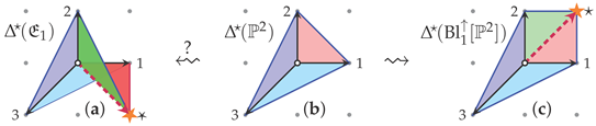
Following the above practice, consider for illustration a simple, two-dimensional version of Greene–Plesser’s 1990 construction [91], a Fermat cubic in (see Figure 2), where the (10)-like fan was redrawn in Figure 2b in the customary orientation and labeled by the Cox coordinates, so powers of in the Newton polytope, Figure 2a, grow in the direction of the -arrow in . This fan subdivides its “spanning polytope”, . The “original” Calabi–Yau 1-fold is simply the zero locus of the Fermat cubic Figure 2 (top left), . The Greene–Plesser mirror was then defined as a Calabi–Yau desingularization of a -quotient of the same cubic in essentially the same .

Figure 2.
Combinatorial data for as a toric variety, and for : the Newton polygon of (regular) anticanonical monomials (a), in Cox coordinates specified by the spanning polygon and fan , (b). Similarly, Newton polygon in (c) and spanning polygon and fan in (d). The colored lines in diagrams (a,c) indicate “stripes” of monomials as in Figure 1 and also outline the respective Newton polygons, and .
In Figure 2b, this mirror quotient of the Fermat cubic is seen as the transpose (the matrix of exponents is self-transposed), combining monomials from the Newton polytope, Figure 2c, given in terms of a distinct set of variables, , specified by the fan of a distinct embedding space, , depicted in Figure 2d. As should be clear from the shapes in Figure 2, this implements mirror symmetry by swapping the roles of the spanning polytope, , and the Newton polytope, . That is,
where the “original” is an anticanonical hypersurface in X and its mirror is a corresponding hypersurface in , which is specified by both and , as defined in (55). This in fact automagically incorporates the requisite quotient desingularization, as seen after a brief toric précis (see Refs. [47,48,49,70,71,72] for rigorous and complete details).
- Cox coordinates:
- Chart:
- A toric variety, X, is covered by an atlas of chars, each corresponding to a top-dimensional cone in the fan, . The lattice degree of a cone, , is the dimension-rescaled volume of the 0-apex pyramid generated by the cone’s lattice-primitive generators: .
- MPCP-desingularization:
- Degree-d cones encode -like affine charts (), a maximal projective crepant partial (MPCP)-desingularization (blowup) [92] of which is encoded by a subdivision into degree-1 subcones; each generator cone of the subdivision encodes (part of) an exceptional locus of the MPCP-desingularization.
- Charts and gluing:
- A toric variety, X is covered by an atlas of chars, each corresponding to a top-dimensional cone in the fan, . Charts overlap where their (top-dimensional) cones have a common facet (codimension-1 cone in the boundary), which then specifies how the charts are glued together. The so-defined poset structure in the atlas of charts covering X is in direct 1–1 correspondence to the poset of cones in the fan . A complete fan (where each codimension-1 facet adjoins two top-dimensional cones) corresponds to a compact toric space.
- Multifan layers:
- In multifans (as used in Refs. [60,61,62,63]), a common facet -cone, , adjoins two k-cones, that lie in distinct layers of a multifan that “flip-folds” at , so that contrary to appearances of a larger overlap. The hyperplane region spanned by the lattice-primitive generators of a cone is its (base) face in the spanning multitope of the multifan, which is assembled from the faces of all the cones and with the same poset structure; a precise correspondence with the rich (and varied) practices in the mathematical literature [70,71,72,73,74,75,76,77,78,79,80,81,94] remains to be determined.
Now, compare in Figure 2b with in Figure 2d. Each of the three top-dimensional cones of in Figure 2b has a degree of 1 [15]:
so each encodes the familiar -like chart, which jointly cover . By contrast, each of the three top-dimensional cones of in Figure 2d has a degree of 3:
They all encode identical -like charts, which jointly cover , thereby indicating the global quotient, . Each chart requires two MPCP-desingularizing blowups, corresponding to the dotted lines in Figure 2d: .
This Figure 2d-encoded quotienting and MPCP-desingularization in is “inherited” by the hypersurface , where it precisely matches the complete Greene–Plesser prescription [91]. Indeed, the Newton polytope consists only of monomials that are invariant under the action (This is precisely the analogue of the Greene–Plesser choice, and is obtained as follows. Start with a generic diagonal action , where the invariance of the individual cubes requires . The invariance of the fundamental monomial, , (oft-quoted as “the Calabi–Yau condition”) sets . The overall projectivization subsumes the choice, , leaving the equivalent choices, , , and with , as the remaining candidates).
Corollary 2.
The zero locus of the transpose anticanonical section, , with the toric space encoded by the fan that star-subdivides and by , requires neither further quotienting nor any desingularization: is already well prepared, including all requisite MPCP-desingularization of all -encoded local quotient singularities.
3.2. Simplicial Reductions
Generalizations of the Greene-Plesser construction to other types of transverse defining Equations (with a minimal number of monomials) á la [55] is then depicted by simplicial 0-enclosing reductions of the Newton polytope, depicted for (and dually, for ) in Figure 3, where the (bigger, pale blue) Newton triangle, , is depicted over the (smaller, yellow) triangle, . The thicker (green) triangles outline the encode the defining polynomial underneath it, with the Refs. [55,95]-styled depiction underneath that; Arnold’s original classification [95] guarantees completeness.
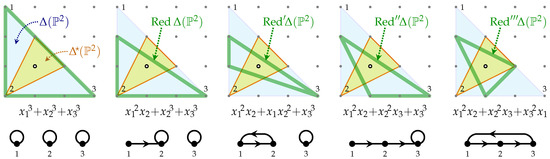
Figure 3.
The distinct types of transverse cubics [95], classified as distinct simplicial 0-enclosing reductions of the complete Newton polytope. The variously colored triangles and their relation to the polynomials and graphs underneath are specified in the text, just above the figure.
The combinatorially generated collection of different possible simplicial reductions evidently grows fast with the dimension and complexity of the considered polytope pairs, . Each of these specifies a mirror pair of Calabi–Yau manifolds. They are related by the fact that varying the reduction corresponds to a deformation of the chosen defining equation, i.e., to a deformation of the complex structure, —both of which are mirrors to the “same ”, held “fixed” by not changing . Since of the embedding space, X, of the “original”, is the spanning polytope of the embedding space, , of the “transposition-mirror”, , varying then also corresponds to varying the Kähler class (and also the symplectic structure [96,97]!) of , which are, thus, “held fixed” as a complex manifold—up to Bridgeland stability issues that make the choice of the complex and the Kähler structures subtly codependent [98]. In this sense, Corollary 3 holds.
Corollary 3.
The original, unreduced polytope pair, , may be regarded as encoding a “generating machine” for (“multiple”) mirror model pairs.
3.3. Flip-Folded Layers
As the comparison of the two plots in Figure 1 indicates, extending the foregoing description of the transposition-mirror construction to hypersurfaces in defines the embedding space, , of the mirror model by the defining identities (55). To this end, it is of key importance that the relation between the Newton and spanning polytope, such as , is constructed using the (GLSM-deformation motivated) “stripe”-wise computed transpolar operation—rather than the algebraic-geometry standard, global, polar operation. This “stripe”-wise local computation makes the transpolar operation expressly sensitive to all forms of non-convexity, such as evident in (10, b)—which the global computations in the standard polar operation obscure.
Abstracting from the plot in Figure 1b and adapting the diagram (10, b) to the toric style of Figure 2 results in the double-duty diagrams in Figure 4.
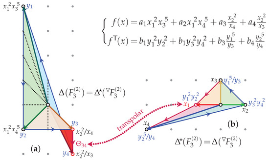
Figure 4.
Combinatorial data for and : on the left, (a), and on the right, (b); the transpose pair of “cornerstone” defining polynomials is given (top right) in terms of Cox coordinates and monomials specified by the vertices.
In Figure 4, and are limited to the “cornerstone” monomials corresponding to the vertices of and , respectively. The matrix of exponents of one is the transpose of that of the other, and they are transverse polynomials provided for , and and for . Relying on Corollary (2), this produces a mirror-pair of zero loci:
However, we still need to better understand the toric space corresponding to . To this end, a few observations are in order, which are easy to generalize for all :
- The dotted lines in the diagram indicate the MPCP-desingularizations, so is a smooth manifold, but it does not stem from a global finite quotient. Corresponding to the four big (vertex-generated) cones, the four distinct charts (starting from the top-left vertex) correspond to the distinct MPCP desingularizations:
- has a maximal toric -action and a (1)-like GLSM specification:
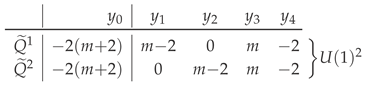 All other linear combinations with integral charges are, for , non-negative linear combinations of and , which are, thereby, the Mori vectors.
 - The gluing and are, however, non-standard. In Figure 4a, the corresponding cones and (as well as and ) seem to partially overlap. This is a hallmark of multifans [70,71,72], which in general correspond to torus manifolds, and which are not algebraic varieties unless the multifan is in fact a (flat) fan.
- The multifan defined by the collection of central cones over the facets (“stripes” of anticanonical monomials that are independent of one of the Cox coordinates) is well defined as a poset if the cone is understood to flip-fold, into a (Riemann-sheet like) layer under and over the layer of . This way, and are 1-cones, consistently extending the “Separation Lemma” [48,49].
- This flip-folded character of the multifan centrally spanned by the multilayered multigonal object , which it star-subdivides, is well encoded by the continuous orientation of the closed cycle of cones,This is a key characteristic of the “generalized legal loops” [99], which in fact are the two-dimensional so-called VEX multitopes [60,61,62], the latter defined so that the transpolar operation acts within their class and always as an involution. Thereby, VEX multitopes and their (local) transpolar involution generalize (in a GLSM-motivated fashion) both (1) the (convex) reflexive polytopes [92] and their (standard, global) polar operation to non-convex, flip-folded, and otherwise multilayered VEX multitopes, as well as (2) the “generalized legal loops” and their (local) dual operation of Ref. [99] to all higher dimensions.
- Multifans do not uniquely encode torus manifolds, but it is not known how the continuous orientation of multifans and multitopes (item 5, above), such as depicted in Figure 4, correlates with various combinatorial data considered in the literature to more precisely specify the available choices among (unitary) torus manifolds.
In general, unitary torus manifolds, multifans, and related combinatorial data corresponding to multilayered multihedral complexes [70,71,72,73,74,75,76,77] (see also [78,79,80,81]) not only do not correspond complex algebraic varieties, but need not admit even an almost complex structure. The relatively simple, flip-folded multifans, such as the illustration in Figure 4a, may well encode a “wrong” sort of a blowup. The blowup of at a (smooth) point is depicted in toric geometry by the right-hand side subdividing operation:
 In this (standard) blowup, depicted in (62, c), the subdividing generator (dashed arrow) in the fan/spanning polytope lies within the cone being subdivided, here . Flip-folding this into a multifan/multitope, depicted in (62, a), of the kind seen in Figure 4a effectively moves the subdividing generator from “⋆” at to “
 ” at —which is outside the cone that was being subdivided, and so, might be called a blowout. The 1-point blowup of may also be described as a connected sum , where the orientation of the second copy of has been reversed [100]. The toric diagram in (62, a) may then well correspond to , without which this reversal of orientation on the second copy does not admit a global complex structure (I am indebted to Prof. M. Masuda for suggesting this possibility). This is supported by the computation of the self-intersection of the divisors corresponding to the star-labeled vertices [62]: (1) , as standard for the exceptional divisor in a standard blow-up; (2) [D]2 = +1, which is opposite from the exceptional divisor in a standard blow-up.
” at —which is outside the cone that was being subdivided, and so, might be called a blowout. The 1-point blowup of may also be described as a connected sum , where the orientation of the second copy of has been reversed [100]. The toric diagram in (62, a) may then well correspond to , without which this reversal of orientation on the second copy does not admit a global complex structure (I am indebted to Prof. M. Masuda for suggesting this possibility). This is supported by the computation of the self-intersection of the divisors corresponding to the star-labeled vertices [62]: (1) , as standard for the exceptional divisor in a standard blow-up; (2) [D]2 = +1, which is opposite from the exceptional divisor in a standard blow-up.This mismatch in orientations causes the complex structure of the rest of to degenerate in at the exceptional divisor (corresponding to the 1-cone “*”) and its local neighborhood. The situation is then most suggestively analogous to the degeneration of the symplectic structure in so-called “presymplectic manifolds”, the description of which also uses flip-folded multigons [94]. This correlation with symplectic geometry is of course also motivated by the general notion that mirror symmetry swaps it with complex geometry [96,97], but requires much more detailed analysis and comparison.
Conjecture 3.
Given a Calabi–Yau hypersurface in a non-Fano toric variety X of which the spanning polytope, , is non-convex, (1) the transposition mirror may be found as a (transposed) hypersurface, , in a toric space, , corresponding to a flip-folded spanning multitope, . (2) The toric space is precomplex, as may well be the mirror Calabi–Yau hypersurface in it, , in that their complex structures degenerate at isolated locations corresponding to the flip-folded elements of the spanning multitope, . (It may be possible to find a Calabi–Yau hypersurface that avoids intersecting the complex structure obstruction in ; there is then no reason for not to be complex).
Remark 8.
The properly general class of Calabi–Yau spaces is rarely openly specified, but is in fact certain to include stratified pseudo-manifolds and other “defects”; see, e.g., [26,27,28,29,101]. A corresponding (co)homology theory that is consistent with mirror symmetry and conifold/geometric transitions has been defined in Ref. [28]; see also Refs. [102,103,104,105] for a more recent discussion. In the present context, a - or even fully -equivariant version seems to be required. The “home” for such a structure is presumed to require the derived categories of coherent sheaves and (special) Lagrangian submanifolds [98].
Let us conclude with the observation that the “flip-foldedness” is not “undone” by straightforward algebro-geometric means, such as a blowdown, i.e., the corresponding removal of one of the “offending” 1-cones while fixing all other features. For example, the flip-folded cone has (at ) as one of its generators, which may be thought of as a (62, a)-styled “outside” subdivision of the cone , and so, a “blowout”, as discussed below (62). Collapsing its exceptional divisor encoded by (while holding fixed all cones not adjacent to ) converts the flip-folded into a flat (simple, single-layered) albeit non-convex polygon. However, its “stripe”-wise locally computed transpolar is now flip-folded:
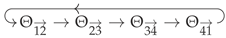
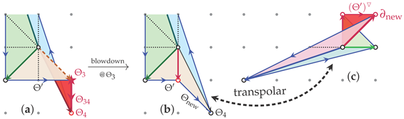 That is, unfolding ends up flip-folding via their transpolar relationship.
Corollary 4.
The transpolar image of a non-convex region is a flip-folded region, and vice versa.
Here, the so-introduced edge, , encodes the pair of anticanonical monomials, , which does not belong to any of the -deformation defined “stripes” nor does it otherwise relate to the GLSM. Dually, the direction in (63, c) does not indicate any of the characteristic deformations of the fundamental monomial, , in the plot of monomials in Figure 1b. The analogous blowdown at has identical consequences. After hand modification, the pair corresponds to ; they encode some different toric spaces.
The above-motivated need to extend reflexive polytopes [92] so as to include flip-folded and otherwise multilayered polyhedral objects (see also [106]) motivates a vast extension of the existing GLSM-motivated applications of toric geometry to follow Definition 2.
Definition 2
([62]). An L-lattice VEX multitope, , is a continuously orientable, possibly multilayered, multihedral n-dimensional body with every facet at unit distance [Def. 4.1.4] of [92] from , and is star-triangulated by a 0-centered multifan [72]: is a facet-ordered poset of its 0-centered cones, , where is a facet : and . Then, has the same poset structure.
The toric geometry definition of “unit distance” perfectly corresponds to the -deformation definition of “distance-1”. VEX multitopes were originally introduced [60] in tandem with the transpolar operation (Section 2.1), aiming to satisfy Conjecture 4.
Conjecture 4
([62]). For an L-lattice VEX multitope, Δ: (1) is a VEX multitope; (2) : the transpolar operation (Section 2.1) closes on VEX multitopes as an involution; (3) The star-triangulation of Δ is L-primitive: lattice points of each star-triangulating simplex are only and in ; and, if Δ has a unit-degree triangulation, (4) has a corresponding unit-degree (-)lattice triangulation, so both Δ and correspond to smooth toric spaces.
4. Concerns and Conclusions
The explicit -varying deformations within the double deformation families of Calabi–Yau hypersurfaces in -varying embedding spaces such as discussed in Section 2.3 insure that the so-constructed embedding spaces (here, ) are diffeomorphic to each other [107]. These deformation families also include non-Fano embedding spaces and their “unsmoothable” (here, Tyurin degenerate) Calabi–Yau hypersurfaces.
Our main concern here is whether there exists smoothings that preserve this diffeomorphism equivalence also at the level of the Calabi–Yau hypersurfaces (see [108,109] ) and the anticanonical bundles, . The Laurent deformations and their non-algebraic “intrinsic limit” completion/closure discussed herein would seem to satisfy this requirement, and is supported by a great deal of explicit computations, as reported earlier [60,61,62,63].
The main claims and statements are indicated throughout the foregoing discussion as Corollaries 1–4 and Remarks 1–7. With regard to the smoothing of the “unsmoothable” Tyurin-degenerate models, these all refer to the non-algebraic (and presumably complex-structure degenerating) “intrinsic limit”. The admittedly less completely justified but hopefully well-motivated statements are indicated as Conjectures 1–4, followed in contrast by the decidedly algebro-geometric Conjecture 5 and ensuing questions.
One More Thing: An Algebraic Alternative
Contrasting the non-algebraic smoothing discussed above, let us close with a firmly algebro-geometric alternative: Ref. [61] reported an -generalization of a fractional mapping devised by D. Cox for ; this generalization converts the entire system of anticanonical sections of —including the rational sections discussed here—into the system of regular sections of a different algebraic variety. In fact, this can be generalized to all . Start with the toric specification á la (6), for :
The change of variables (selected to preserve the fibration nature of , from a very wide range of choices)
converts (64) into a completely regular polynomial:
which is a (not completely) generic -section of ; for example, the -term omits factors. Unsurprisingly, this fractional change of variables has a non-constant Jacobian, and is ill-defined over the poles of —very much like (44). However, very much unlike (44), the mapping (65) relates the Laurent, “intrinsic limit”-defined and transversal Calabi–Yau hypersurfaces to regular, transverse hypersurfaces of general type: , which is negative over . Owing to the appearance of both roots and powers in (65), the relationship between and must involve both multiple covers and (presumably a suitable desingularization of) quotients. Any relationship between this “regularizing” change of variables (65) and the geometry of hypersurfaces of general type on one hand and the Laurent-deformed Calabi–Yau models discussed here would seem to be worthwhile. It is likely to provide new information about the novel, Laurent-deformed Calabi–Yau constructions, and perhaps a firmly algebraic reinterpretation of the “intrinsic limit” completion/closure of the Laurent-deformed hypersurfaces.
The relative ease (and the wide degree of freedom) in generalizing Cox’s fractional mapping to the anticanonical system of all motivates:
Conjecture 5
(Regularizing). All Calabi–Yau Laurent hypersurfaces encoded by VEX-multitopes of anticanonical sections are also describable via suitable fractional transformations in terms of general type complete intersections of hypersurfaces in projective spaces, with strictly regular defining polynomials, i.e., sums of monomials with only non-negative powers.
By providing a strictly complex-algebraic bypass around the putative pole-singularity issue in Laurent hypersurfaces, fractional mappings such as (64)–(66) raise obvious questions about the scope, differences, and possible overlap between the distinct logical possibilities (For string theory applications, this requires a (co)homology theory consistent with mirror symmetry and conifold/geometric transitions including various associated “defects” [26,27,28,29], akin to the framework developed in Ref. [28], but with the GLSM - or even full -equivariance incorporated). (1) What is the (co)homological difference from the “intrinsic limit”? (2) Do they remain in the same deformation class (51), or are there “vanishing (or emerging) cycles”? That is, do the Betti or Hodge numbers differ, and how? (3) How does the symplectic structure on these models (and homological mirror symmetry) vary in the deformation process (51)? Eventually and if interested in string theory application, one would need to know: (4) Do the Weil–Petersson–Zamolodchikov metric-normalized Yukawa couplings (structure constants in the multiplicative and cohomology groups) differ, and how? However, answering this question would be a tall order currently.
Funding
This research received no external funding.
Data Availability Statement
The data discussed in this article is contained within the article.
Acknowledgments
First and foremost, I should like to thank B. Park for the kind invitation and opportunity to present this work. I am deeply grateful to Per Berglund for decades of collaborations including on the topics discussed here, and Corollary 2 in particular, to Mikiya Masuda for their explanations of unitary torus manifolds, and to Marco Aldi, Yong Cui, and Amin Gholampour for insightful and instructive discussions. I am grateful to the Mathematics Department of the University of Maryland, and the Physics Department of the University of Novi Sad, Serbia, for recurring hospitality and resources.
Conflicts of Interest
The author declares no conflicts of interest.
Abbreviations
The following abbreviations are used in this manuscript:
| GLSM | Gauged Linear Sigma Model (a class of worldsheet quantum field theories) [24] |
| MPCP | Maximal Projective Crepant Partial (desingularization) [92] |
| VEX | mnemonic contraction for “not necessarily conVEX EXtension”; see Definition 2, originally [60] |
References
- Friedan, D.H. Nonlinear Models in 2+ϵ Dimensions. Phys. Rev. Lett. 1980, 45, 1057. [Google Scholar] [CrossRef]
- Friedan, D.H. Nonlinear Models in 2+ϵ Dimensions. Ann. Phys. 1985, 163, 318–419. [Google Scholar] [CrossRef]
- Polchinski, J. String Theory. Vol. 1: An Introduction to the Bosonic String; Cambridge Monographs on Mathematical Physics; Cambridge University Press: Cambridge, UK, 2007. [Google Scholar] [CrossRef]
- Polchinski, J. String Theory. Vol. 2: Superstring Theory and Beyond; Cambridge Monographs on Mathematical Physics; Cambridge University Press: Cambridge, UK, 2007. [Google Scholar] [CrossRef]
- Frenkel, I.B.; Garland, H.; Zuckerman, G.J. Semiinfinite Cohomology and String Theory. Proc. Nat. Acad. Sci. USA 1986, 83, 8442. [Google Scholar] [CrossRef]
- Bowick, M.J.; Rajeev, S.G. String Theory as the Kahler Geometry of Loop Space. Phys. Rev. Lett. 1987, 58, 535. [Google Scholar] [CrossRef]
- Bowick, M.J.; Rajeev, S.G. The Holomorphic Geometry of Closed Bosonic String Theory and Diff S1/S1. Nucl. Phys. 1987, B293, 348. [Google Scholar] [CrossRef]
- Bowick, M.J.; Rajeev, S. The Complex Geometry of String Theory and Loop Space. In Proceedings of the Johns Hopkins Workshop on Current Problems in Particle Theory, Lanzhou, China, 17–19 June 1987; Duan, Y.S., Domókos, G., Kövesi-Domókos, S., Eds.; World Scientific Publishing: Singapore, 1987. [Google Scholar]
- Oh, P.; Ramond, P. Curvature of Superdiff S1/S1. Phys. Lett. 1987, B195, 130–134. [Google Scholar] [CrossRef]
- Harari, D.; Hong, D.K.; Ramond, P.; Rodgers, V.G.J. The Superstring Diff S1/S1 and Holomorphic Geometry. Nucl. Phys. 1987, B294, 556–572. [Google Scholar] [CrossRef]
- Pilch, K.; Warner, N.P. Holomorphic Structure of Superstring Vacua. Class. Quant. Grav. 1987, 4, 1183. [Google Scholar] [CrossRef]
- Bowick, M.J.; Rajeev, S.G. Anomalies and Curvature in Complex Geometry. Nucl. Phys. 1988, B296, 1007–1033. [Google Scholar] [CrossRef]
- Bowick, M.J.; Lahiri, A. The Ricci Curvature of Diff S1/SL(2, R). J. Math. Phys. 1988, 29, 1979–1981. [Google Scholar] [CrossRef]
- Bowick, M.J.; Yang, K.Q. String Equations of Motion from Vanishing Curvature. Int. J. Mod. Phys. 1991, A6, 1319–1334. [Google Scholar] [CrossRef]
- Hübsch, T. Calabi–Yau Manifolds: A Bestiary for Physicists, 2nd ed.; World Scientific Publishing Europe Ltd.: London, UK, 2024. [Google Scholar]
- Candelas, P.; Horowitz, G.T.; Strominger, A.; Witten, E. Vacuum configurations for superstrings. Nucl. Phys. 1985, B258, 46–74. [Google Scholar] [CrossRef]
- Hull, C.M. Sigma Model Beta Functions and String Compactifications. Nucl. Phys. B 1986, 267, 266–276. [Google Scholar] [CrossRef]
- Strominger, A. Superstrings with Torsion. Nucl. Phys. B 1986, 274, 253. [Google Scholar] [CrossRef]
- Hull, C.M. Compactifications of the Heterotic Superstring. Phys. Lett. B 1986, 178, 357–364. [Google Scholar] [CrossRef]
- Becker, K.; Sethi, S. Torsional Heterotic Geometries. Nucl. Phys. B 2009, 820, 1–31. [Google Scholar] [CrossRef]
- Dasgupta, K.; Rajesh, G.; Sethi, S. M theory, orientifolds and G-flux. J. High Energy Phys. 1999, 8, 023. [Google Scholar] [CrossRef]
- Becker, K.; Becker, M.; Green, P.S.; Dasgupta, K.; Sharpe, E. Compactifications of heterotic strings on non-Kähler complex manifolds II. Nucl. Phys. 2004, B678, 19–100. [Google Scholar] [CrossRef]
- Becker, K.; Becker, M.; Dasgupta, K.; Green, P.S. Compactifications of heterotic theory on non-Kahler complex manifolds, I. J. High Energy Phys. 2003, 4, 007. [Google Scholar] [CrossRef]
- Witten, E. Phases of N = 2 theories in two-dimensions. Nucl. Phys. 1993, B403, 159–222. [Google Scholar] [CrossRef]
- Morrison, D.R.; Plesser, M.R. Summing the instantons: Quantum cohomology and mirror symmetry in toric varieties. Nucl. Phys. 1995, B440, 279–354. [Google Scholar] [CrossRef]
- Aspinwall, P.S.; Greene, B.R.; Morrison, D.R. Calabi–Yau Moduli Space, Mirror Manifolds and Space-Time Topology Change in String Theory. Nucl. Phys. 1994, B416, 414–480. [Google Scholar] [CrossRef]
- Hübsch, T.; Rahman, A. On the geometry and homology of certain simple stratified varieties. J. Geom. Phys. 2005, 53, 31–48. [Google Scholar] [CrossRef]
- Banagl, M. Intersection Spaces, Spatial Homology Truncation, and String Theory; Number 1997 in Lecture Notes in Mathematics; Springer: Berlin/Heidelberg, Germany, 2010. [Google Scholar]
- McNamara, J.; Vafa, C. Cobordism Classes and the Swampland. arXiv 2019, arXiv:1909.10355. [Google Scholar] [CrossRef]
- Berglund, P.; Hübsch, T.; Minic, D. On de Sitter Spacetime and String Theory. Int. J. Mod. Phys. D 2023, 32, 2330002. [Google Scholar] [CrossRef]
- Kasner, E. Finite Representation of the Solar Gravitational Field in Flat Space of Six Dimensions. Am. J. Math. 1921, 43, 130–133. [Google Scholar] [CrossRef]
- Fronsdal, C. Completion and Embedding of the Schwarzschild Solution. Phys. Rev. 1959, 116, 778–781. [Google Scholar] [CrossRef]
- Distler, J.; Kachru, S. (0, 2) Landau–Ginzburg theory. Nucl. Phys. B 1994, 413, 213–243. [Google Scholar] [CrossRef]
- Sharpe, E. A survey of recent developments in GLSMs. Int. J. Mod. Phys. A 2024, 39, 2446001. [Google Scholar] [CrossRef]
- Hübsch, T. Calabi–Yau Manifolds—Motivations and Constructions. Commun. Math. Phys. 1987, 108, 291–318. [Google Scholar] [CrossRef]
- Green, P.S.; Hübsch, T. Calabi–Yau Manifolds as Complete Intersections in Products of Projective Spaces. Comm. Math. Phys. 1987, 109, 99–108. [Google Scholar] [CrossRef]
- Candelas, P.; Dale, A.M.; Lütken, C.A.; Schimmrigk, R. Complete intersection Calabi–Yau manifolds. Nucl. Phys. 1988, B298, 493. [Google Scholar] [CrossRef]
- Candelas, P.; Lynker, M.; Schimmrigk, R. Calabi–Yau Manifolds in Weighted P(4). Nucl. Phys. 1990, B341, 383–402. [Google Scholar] [CrossRef]
- Kreuzer, M.; Skarke, H. On the classification of reflexive polyhedra. Commun. Math. Phys. 1997, 185, 495–508. [Google Scholar] [CrossRef]
- Skarke, H. Weight Systems for Toric Calabi–Yau Varieties and Reflexivity of Newton Polyhedra. Mod. Phys. Lett. A 1996, 11, 1637–1652. [Google Scholar] [CrossRef]
- Kreuzer, M.; Skarke, H. Classification of Reflexive Polyhedra in Three Dimensions. Adv. Theor. Math. Phys. 1998, 2, 853–871. [Google Scholar] [CrossRef]
- Kreuzer, M.; Skarke, H. Complete classification of reflexive polyhedra in four-dimensions. Adv. Theor. Math. Phys. 2000, 4, 1209–1230. [Google Scholar] [CrossRef]
- Kreuzer, M.; Skarke, H. Calabi–Yau Data. Available online: http://hep.itp.tuwien.ac.at/~kreuzer/CY/ (accessed on 25 January 2025).
- Constantin, A.; He, Y.H.; Lukas, A. Counting String Theory Standard Models. Phys. Lett. B 2019, 792, 258–262. [Google Scholar] [CrossRef]
- Griffiths, P.; Harris, J. Principles of Algebraic Geometry; Wiley Classics Library; John Wiley & Sons Inc.: New York, NY, USA, 1978. [Google Scholar]
- Danilov, V.I. The Geometry of Toric Varieties. Russ. Math. Surv. 1978, 33, 97–154. [Google Scholar] [CrossRef]
- Fulton, W. Introduction to Toric Varieties; Annals of Mathematics Studies; Princeton University Press: Princeton, NJ, USA, 1993. [Google Scholar]
- Ewald, G. Combinatorial Convexity and Algebraic Geometry; Springer: Berlin/Heidelberg, Germany, 1996. [Google Scholar]
- Cox, D.A.; Little, J.B.; Schenck, H.K. Toric Varieties; Graduate Studies in Mathematics; American Mathematical Society: Providence, RI, USA, 2011; Volume 124, Available online: https://www.mimuw.edu.pl/~jarekw/pragmatic2010/CoxLittleSchenckJan2010.pdf (accessed on 18 March 2025).
- Brooks, R.; Muhammad, F.; Gates, S.J., Jr. Unidexterous D = 2 Supersymmetry in Superspace. Nucl. Phys. 1986, B268, 599–620. [Google Scholar]
- Brooks, R.; Gates, S.J., Jr. Unidexterous D = 2 Supersymmetry in Superspace. 2. Quantization. Phys. Lett. 1987, B184, 217. [Google Scholar]
- Gates, S.J., Jr.; Brooks, R.; Muhammad, F. Unidexterous Superspace: The Flax of (Super)Strings. Phys. Lett. 1987, B194, 35. [Google Scholar]
- Gates, S.J., Jr.; Hübsch, T. Calabi–Yau Heterotic Strings and Unidexterous Sigma Models. Nucl. Phys. 1990, B343, 741–774. [Google Scholar] [CrossRef]
- Kusuki, Y. Modern Approach to 2D Conformal Field Theory. arXiv 2024, arXiv:2412.18307. [Google Scholar] [CrossRef]
- Berglund, P.; Hübsch, T. A generalized construction of mirror manifolds. Nucl. Phys. 1993, B393, 377–391. [Google Scholar] [CrossRef]
- Berglund, P.; Henningson, M. Landau–Ginzburg orbifolds, mirror symmetry and the elliptic genus. Nucl. Phys. 1995, B433, 311–332. [Google Scholar] [CrossRef]
- Krawitz, M.; Priddis, N.; Acosta, P.; Bergin, N.; Rathnakumara, H. FJRW-Rings and Mirror Symmetry. Comm. Math. Phys. 2009, 296, 145–174. [Google Scholar] [CrossRef]
- Borisov, L.A. Berglund-Hübsch mirror symmetry via vertex algebras. Comm. Math. Phys. 2013, 320, 73–99. [Google Scholar] [CrossRef]
- Berglund, P.; Hübsch, T. On Calabi–Yau generalized complete intersections from Hirzebruch varieties and novel K3-fibrations. Adv. Theor. Math. Phys. 2018, 22, 261–303. [Google Scholar] [CrossRef]
- Berglund, P.; Hübsch, T. A Generalized Construction of Calabi–Yau Models and Mirror Symmetry. SciPost 2018, 4, 9. [Google Scholar] [CrossRef]
- Berglund, P.; Hübsch, T. Hirzebruch Surfaces, Tyurin Degenerations and Toric Mirrors: Bridging Generalized Calabi–Yau Constructions. Adv. Theor. Math. Phys. 2022, 26, 2541–2598. [Google Scholar] [CrossRef]
- Berglund, P.; Hübsch, T. Chern Characteristics and Todd–Hirzebruch Identities for Transpolar Pairs of Toric Spaces. arXiv 2024, arXiv:2403.07139. [Google Scholar] [CrossRef]
- Hübsch, T. Ricci–Flat Mirror Hypersurfaces in Spaces of General Type. In Proceedings of the 11th Mathematical Physics Meeting, Belgrade, Serbia, 2–6 September 2024. [Google Scholar]
- Hirzebruch, F. Über eine Klasse von einfach-zusammenhängenden komplexen Mannigfaltigkeiten. Math. Ann. 1951, 124, 77–86. [Google Scholar]
- Gates, S.J., Jr.; Hübsch, T. Unidexterous Locally Supersymmetric Actions For Calabi–Yau Compactifications. Phys. Lett. 1989, B226, 100. [Google Scholar] [CrossRef]
- Hübsch, T. Chameleonic Sigma-Models. Phys. Lett. 1990, B247, 317–322. [Google Scholar] [CrossRef]
- Hübsch, T. How Singular a Space can Superstrings Thread? Mod. Phys. Lett. 1991, A6, 207–216. [Google Scholar] [CrossRef]
- Hübsch, T.; Yau, S.T. An SL(2,C) action on chiral rings and the mirror map. Mod. Phys. Lett. 1992, A7, 3277–3289. [Google Scholar] [CrossRef]
- Berglund, P.; Candelas, P.; de la Ossa, X.; Font, A.; Hübsch, T.; Jancic, D.; Quevedo, F. Periods for Calabi–Yau and Landau–Ginzburg Vacua. Nucl. Phys. 1994, B419, 352–403. [Google Scholar] [CrossRef]
- Masuda, M. Unitary toric manifolds, multi-fans and equivariant index. Tohoku Math. J. (2) 1999, 51, 237–265. [Google Scholar] [CrossRef]
- Masuda, M. From Convex Polytopes to Multi-Polytopes. Notes Res. Inst. Math. Anal. 2000, 1175, 1–15. [Google Scholar]
- Hattori, A.; Masuda, M. Theory of Multi-Fans. Osaka J. Math. 2003, 40, 1–68. [Google Scholar]
- Masuda, M.; Panov, T. On the cohomology of torus manifolds. Osaka J. Math. 2006, 43, 711–746. [Google Scholar]
- Hattori, A.; Masuda, M. Elliptic genera, torus manifolds and multi-fans. Int. J. Math. 2006, 16, 957–998. [Google Scholar] [CrossRef]
- Hattori, A. Elliptic genera, torus orbifolds and multi-fans; II. Int. J. Math. 2006, 17, 707–735. [Google Scholar] [CrossRef]
- Nishimura, Y. Multipolytopes and Convex Chains. Proc. Steklov Inst. Math. 2006, 252, 212–224. [Google Scholar] [CrossRef]
- Ishida, H. Invariant Stably Complex Structures on Topological Toric Manifolds. Osaka J. Math. 2013, 50, 795–806. [Google Scholar]
- Davis, M.W.; Januszkiewicz, T. Convex Polytopes, Coxeter Orbifolds and Torus Actions. Duke Math. J. 1991, 62, 417–451. [Google Scholar] [CrossRef]
- Ishida, H.; Fukukawa, Y.; Masuda, M. Topological toric manifolds. Mosc. Math. J. 2013, 13, 57–98. [Google Scholar] [CrossRef]
- Buchstaber, V.; Panov, T. Toric Topology; Number 204 in Mathematical Surveys and Monographs; American Mathematical Society: Providence, RI, USA, 2015. [Google Scholar]
- Jang, D. Four dimensional almost complex torus manifolds. arXiv 2023, arXiv:2310.11024. [Google Scholar] [CrossRef]
- Berglund, P.; Hübsch, T. On a Residue Representation of Deformation, Koszul and Chiral Rings. Int. J. Mod. Phys. A 1995, 10, 3381–3430. [Google Scholar] [CrossRef]
- Hori, K.; Knapp, J. A pair of Calabi–Yau manifolds from a two parameter non-Abelian gauged linear sigma model. arXiv 2016, arXiv:1612.06214. [Google Scholar] [CrossRef]
- Ruan, Y. Nonabelian gauged linear sigma model. Chin. Ann. Math. Ser. B 2017, 38, 963–984. [Google Scholar] [CrossRef]
- Anderson, L.B.; Apruzzi, F.; Gao, X.; Gray, J.; Lee, S.J. A New Construction of Calabi–Yau Manifolds: Generalized CICYs. Nucl. Phys. 2016, B906, 441–496. [Google Scholar] [CrossRef]
- Garbagnati, A.; van Geemen, B. A remark on generalized complete intersections. Nucl. Phys. 2017, B925, 135–143. [Google Scholar] [CrossRef]
- Kodaira, K.; Spencer, D.C. On Deformations of Complex Analytic Structures; Princeton University: Princeton, NJ, USA, 1957; pp. 328–401. [Google Scholar]
- Wall, C.T.C. Classifications Problems in Differential Topology V: On Certain 6-Manifolds. Invent. Math. 1966, 1, 355–374. [Google Scholar] [CrossRef]
- Tian, G.; Yau, S.T. Complete Kähler manifolds with zero Ricci curvature. I. J. Am. Math. Soc. 1990, 3, 579–609. [Google Scholar] [CrossRef]
- Tian, G.; Yau, S.T. Complete Kähler manifolds with zero Ricci curvature. II. Invent. Math. 1991, 106, 27–60. [Google Scholar] [CrossRef]
- Greene, B.R.; Plesser, M.R. Duality in Calabi–Yau Moduli Space. Nucl. Phys. 1990, B338, 15–37. [Google Scholar] [CrossRef]
- Batyrev, V.V. Dual polyhedra and mirror symmetry for Calabi–Yau hypersurfaces in toric varieties. J. Algebr. Geom. 1994, 3, 493–535. [Google Scholar]
- Cox, D.A. The Homogeneous Coordinate Ring of a Toric Variety. J. Algebr. Geom. 1995, 4, 17–50, Erratum in J. Algebr. Geom. 2014, 23, 393–398. [Google Scholar]
- Karshon, Y.; Tolman, S. The moment map and line bundles over presymplectic toric manifolds. J. Diff. Geom. 1993, 38, 465–484. [Google Scholar] [CrossRef]
- Arnold, V.; Gusein-Zade, S.; Varchenko, A. Singularities of Differentiable Maps; Birkhäuser: Boston, MA, USA, 1985; Volume 1. [Google Scholar]
- Kontsevich, M. Homological Algebra of Mirror Symmetry. In Proceedings of the International Congress of Mathematicians; Chatterji, S.D., Ed.; Birkhäuser Basel: Basel, Switzerland, 1995; pp. 120–139. [Google Scholar]
- Kontsevich, M. Mirror symmetry in dimension 3. Astérisque 1996, 237, 275–293. [Google Scholar]
- Aspinwall, P.S.; Bridgeland, T.; Craw, A.; Douglas, M.R.; Kapustin, A.; Moore, G.W.; Gross, M.; Segal, G.; Szendroi, B.; Wilson, P.M.H. Dirichlet Branes and Mirror Symmetry; Clay Mathematics Monographs; AMS: Providence, RI, USA, 2009; Volume 4. [Google Scholar]
- Poonen, B.; Rodriguez-Villegas, F. Lattice Polygons and the Number 12. Am. Math. Mon. 2000, 107, 238–250. [Google Scholar] [CrossRef]
- Huybrechts, D. Complex Geometry; Springer: Berlin/Heidelberg, Germany, 2005. [Google Scholar] [CrossRef]
- Rahman, A. A Perverse Sheaf Approach Toward a Cohomology Theory for String Theory. Adv. Theor. Math. Phys. 2009, 13, 667–693. [Google Scholar] [CrossRef]
- Collins, T.C.; Gukov, S.; Picard, S.; Yau, S.T. Special Lagrangian cycles and Calabi–Yau transitions. Comm. Math. Phys. 2023, 401, 769–802. [Google Scholar] [CrossRef]
- Anderson, L.B.; Brodie, C.R.; Gray, J. Branes and Bundles through Conifold Transitions and Dualities in Heterotic String Theory. Phys. Rev. D 2023, 108, 106019. [Google Scholar]
- Friedman, B.; Picard, S.; Suan, C. Gromov–Hausdorff continuity of non-Kähler Calabi–Yau conifold transitions. arXiv 2024, arXiv:2404.11840. [Google Scholar] [CrossRef]
- Picard, S. Calabi–Yau threefolds across quadratic singularities. arXiv 2025, arXiv:2501.19313. [Google Scholar] [CrossRef]
- Hibi, T. Star-Shaped Complexes and Ehrhart Polynomials. Proc. Am. Math. Soc. 1995, 123, 723–726. [Google Scholar] [CrossRef]
- Kodaira, K. Complex Manifolds and Deformations of Complex Structures; Springer: New York, NY, USA, 1986; pp. 43–76. [Google Scholar] [CrossRef]
- Reid, M.A. The moduli space of 3-folds with K = 0 may nevertheless be irreducible. Math. Ann. 1987, 278, 329–334. [Google Scholar] [CrossRef]
- Friedman, R. On threefolds with trivial canonical bundle. In Complex Geometry and Lie Theory; Carlson, J.A., Clemens, C.H., Morrison, D.R., Eds.; American Mathematical Society: Providence, RI, USA, 1991; Volume 53, pp. 103–134. [Google Scholar] [CrossRef]

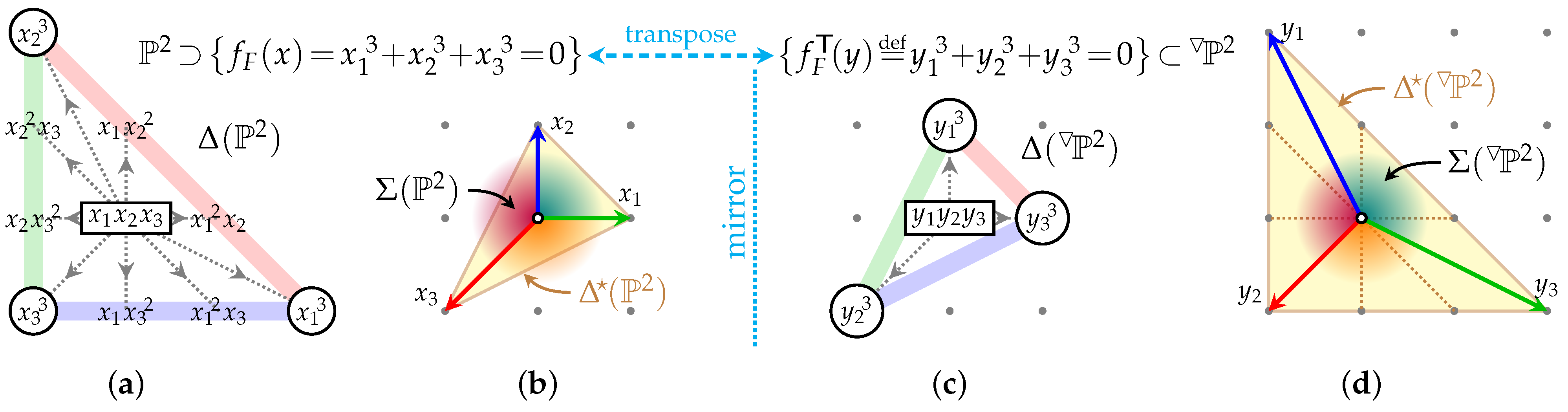
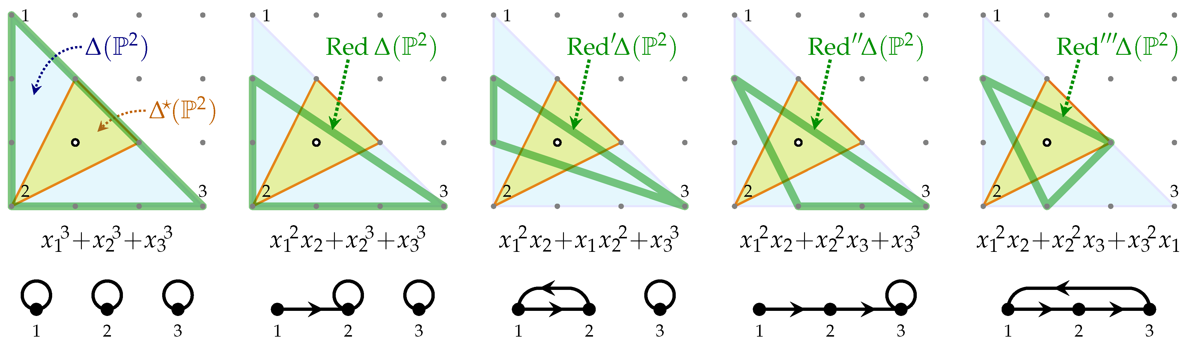
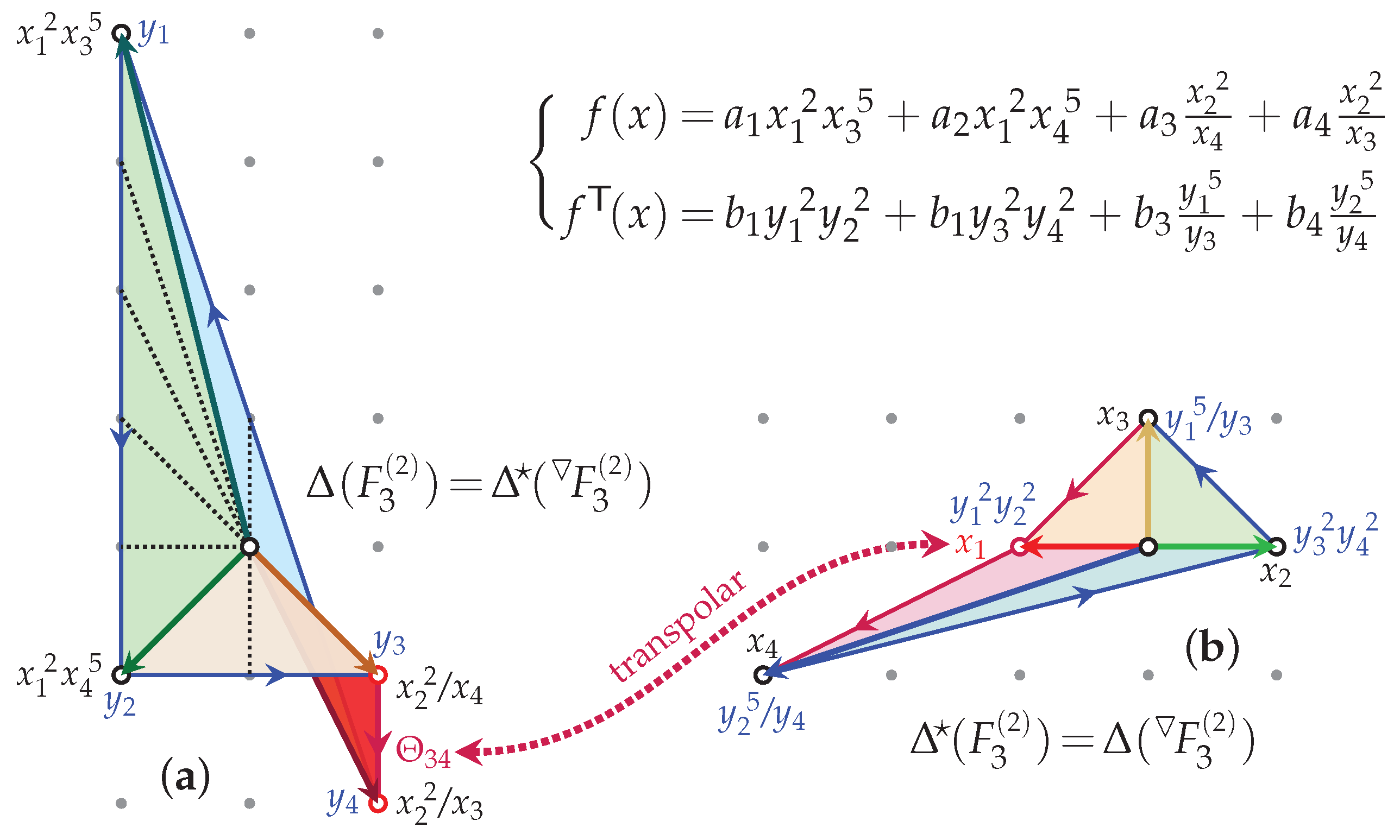
Disclaimer/Publisher’s Note: The statements, opinions and data contained in all publications are solely those of the individual author(s) and contributor(s) and not of MDPI and/or the editor(s). MDPI and/or the editor(s) disclaim responsibility for any injury to people or property resulting from any ideas, methods, instructions or products referred to in the content. |
© 2025 by the author. Licensee MDPI, Basel, Switzerland. This article is an open access article distributed under the terms and conditions of the Creative Commons Attribution (CC BY) license (https://creativecommons.org/licenses/by/4.0/).