
Efficient Layer-Resolving Fitted Mesh Finite Difference Approach for Solving a System of n Two-Parameter Singularly Perturbed Convection–Diffusion Delay Differential Equations

 ,
,  ,
,  and
and
Abstract
1. Introduction
2. Formulation of the Problem
3. Analytical Results
- Claim (i): . If , thenwhich contradicts the assumption that on . Thus, .
- Claim (ii): . If , thenwhich contradicts the assumption that on . Hence, . When , the differentiability of at . If does not exist, then , which contradicts the condition . If is differentiable at , then Since all entries of , and are continuous on , there exists an interval whereNext, the second derivative is examined. If for any , then , which leads to a contradiction. Therefore, we assume on the interval . This indicates that is strictly decreasing over . Given that and is continuous on , it follows that on . As a result, the continuous function cannot attain a minimum at , which contradicts the assumption that . Thus, on . The proof of the lemma is completed. □
4. Shishkin Decomposition of the Solution
- Case (i):
- Case (ii):
5. Bounds on the Regular Component and Its Derivatives
- Case (i):
- Case (ii):
6. Layer Functions
7. Bounds on the Singular Component and Its Derivatives
8. Sharper Bounds for and
9. Numerical Method
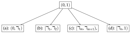
Shishkin Mesh
- Case (i):
- Case (ii):
10. The Discrete Problem
11. Theoretical Analysis and Error Estimation
Error Estimate
 In each scenario, the local truncation error is first estimated. This is followed by the formulation of a suitable barrier function, designed to capture the essential properties of the solution within a specified domain. By utilizing these barrier functions, the desired estimate is obtained.
- Case (a):.
- Case (b):.
- Case (c): .
- Case (c3):. In the previous arguments of Case (c2), by replacing q with m and applying the inequality , the estimates are valid for .For , we haveand, for , we haveFor , defineand, for , define
- Case (d):
 In each scenario, the local truncation error is first estimated. This is followed by the formulation of a suitable barrier function, designed to capture the essential properties of the solution within a specified domain. By utilizing these barrier functions, the desired estimate is obtained.
- Case (a):.
- Case (b):
- Case (b2): . Tor this case, . Hence, for , by utilizing the standard approach to local truncation errors in Taylor series expansions, the term . Then, using Lemma 4, we have
- Case (c): .
- Case (c2): and for some q, . Since , the mesh is uniform in , which implies that , for . The approach to local truncation is derived from Taylor expansions, and it is outlined in Lemma 4, as follows:
- Case (c3): . In the previous arguments of Case (c2), by replacing q with m and applying the inequality , the estimates are valid for .
- Case (d): There are three distinct cases that need to be considered: Case (d1): , Case (d2): and for some q, and Case (d3): . Case (d1): . In this case, the mesh is uniformly distributed over the interval . The corresponding result for this situation is derived in Lemma 9. Case (d2): and for some q, . For this scenario, based on the definition of , it can be shown that Moreover, by employing arguments analogous to Case (c2), this leads to the estimates for . Case (d3): . Let be defined as on the interval . Hence, . Similarly,. Therefore,The proof of the lemma is completed. □
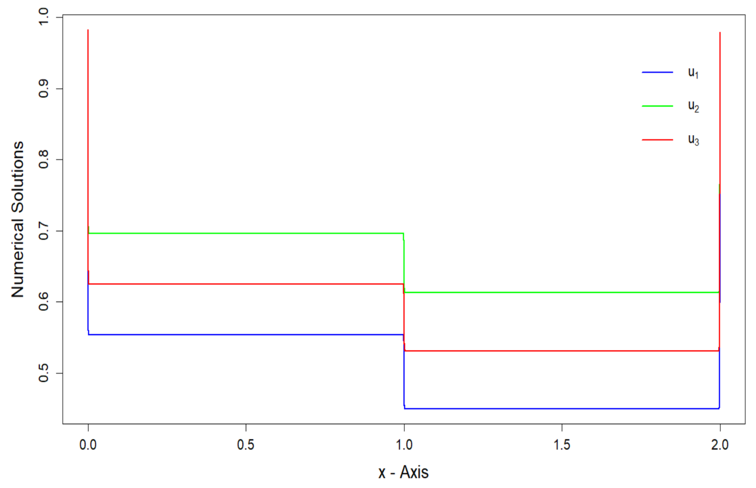
12. Numerical Illustration
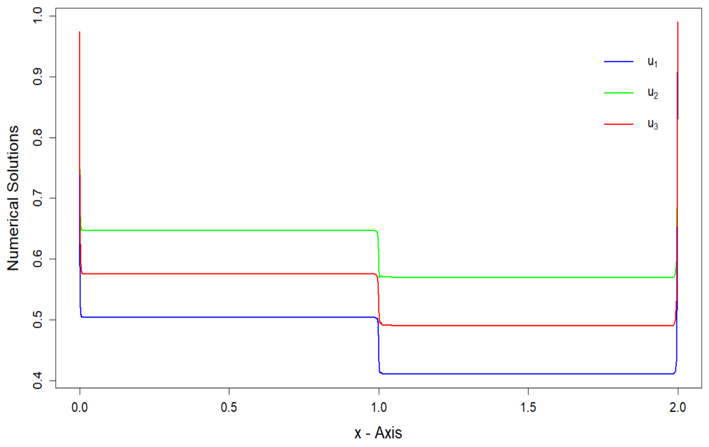
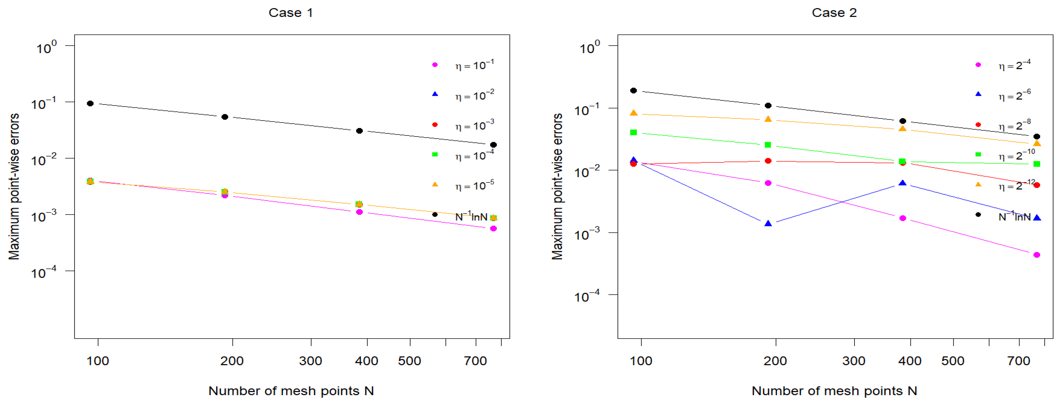
12.1. Example
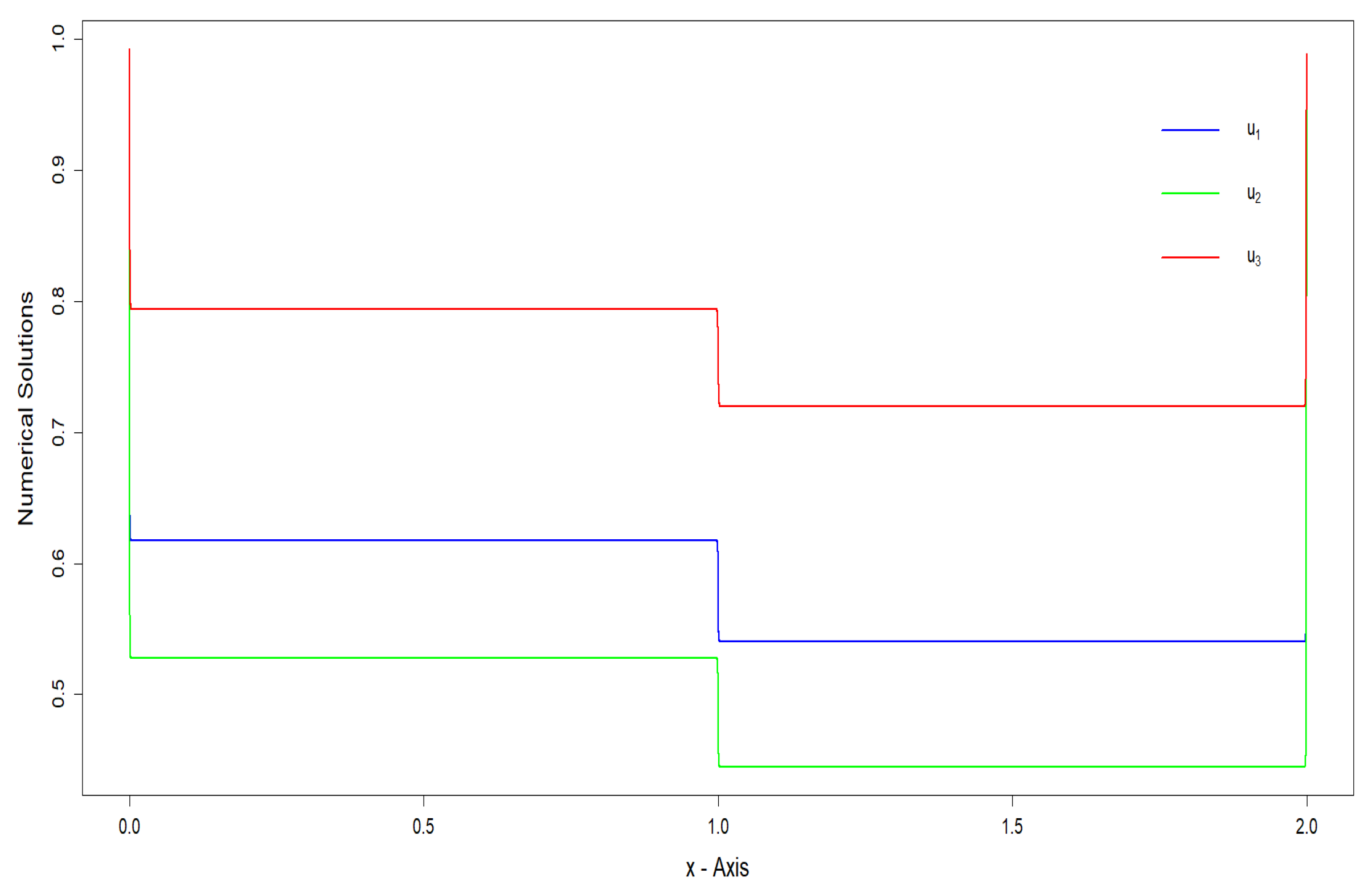
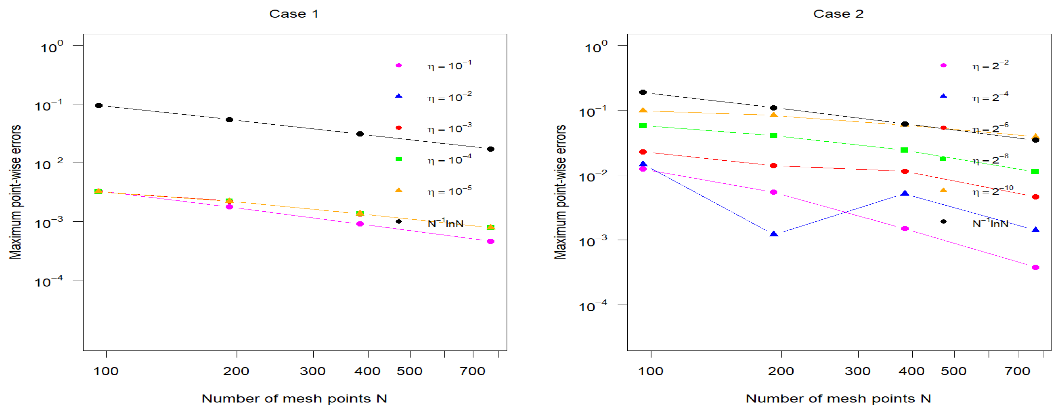
12.2. Example
13. Conclusions
Author Contributions
Funding
Data Availability Statement
Conflicts of Interest
References
- Bhatti, M.M.; Alamri, S.Z.; Ellahi, R.; Abdelsalam, S.I. Intra-uterine particle-fluid motion through a compliant asymmetric tapered channel with heat transfer. J. Therm. Anal. Calorim. 2021, 144, 2259–2267. [Google Scholar] [CrossRef]
- Glizer, V. Asymptotic analysis and solution of a finite-horizon H∞ control problem for singularly-perturbed linear systems with small state delay. J. Optim. Theory Appl. 2003, 117, 295–325. [Google Scholar] [CrossRef]
- Miller, J.J.H.; O’Riordan, E.; Shishkin, G.I. Fitted Numerical Methods for Singular Perturbation Problems: Error Estimates in the Maximum Norm for Linear Problems in One and Two Dimensions; World Scientific: Singapore, 2012. [Google Scholar]
- Doolan, E.P.; Miller, J.J.H.; Schilders, W.H.A. Uniform Numerical Methods for Problems with Initial and Boundary Layers; Boole Press: Dublin, Ireland, 1980. [Google Scholar]
- Cen, Z. Parameter-uniform finite difference scheme for a system of coupled singularly perturbed convection-diffusion equations. Int. J. Comput. Math. 2005, 82, 177–192. [Google Scholar] [CrossRef]
- Gracia, J.L.; O’Riordan, E.; Pickett, M.L. A parameter robust second order numerical method for a singularly perturbed two-parameter problem. Appl. Numer. Math. 2006, 56, 962–980. [Google Scholar] [CrossRef]
- O’Malley, R.E. Two-parameter singular perturbation problems for second-order equations. J. Math. Mech. 1967, 16, 1143–1164. [Google Scholar]
- O’Riordan, E.; Pickett, M.L.; Shishkin, G.I. Singularly perturbed problems modeling reaction-convection-diffusion processes. Comput. Methods Appl. Math. 2003, 3, 424–442. [Google Scholar] [CrossRef]
- Raja, V.; Geetha, N.; Mahendran, R.; Senthilkumar, L.S. Numerical solution for third order singularly perturbed turning point problems with integral boundary condition. J. Appl. Math. Comput. 2025, 71, 829–849. [Google Scholar] [CrossRef]
- Besova, M.; Kachalov, V. Axiomatic approach in the analytic theory of singular perturbations. Axioms 2020, 9, 9. [Google Scholar] [CrossRef]
- Daba, I.T.; Melesse, W.G.; Gelu, F.W.; Kebede, G.D. An efficient numerical approach for singularly perturbed time delayed parabolic problems with two parameters. BMC Res. Notes 2024, 17, 158. [Google Scholar] [CrossRef]
- Woldaregay, M.M. Solving singularly perturbed delay differential equations via fitted mesh and exact difference method. Res. Math. 2022, 9, 2109301. [Google Scholar] [CrossRef]
- Kalaiselvan, S.S.; Miller, J.J.H.; Sigamani, V. A parameter uniform numerical method for a singularly perturbed two-parameter delay differential equation. Appl. Numer. Math. 2019, 145, 90–110. [Google Scholar] [CrossRef]
- Nagarajan, S. A parameter robust fitted mesh finite difference method for a system of two reaction-convection-diffusion equations. Appl. Numer. Math. 2022, 179, 87–104. [Google Scholar] [CrossRef]
- Arthur, J.; Chatzarakis, G.E.; Panetsos, S.L.; Mathiyazhagan, J.P. A robust-fitted-mesh-based finite difference approach for solving a system of singularly perturbed convection–diffusion delay differential equations with two parameters. Symmetry 2025, 17, 68. [Google Scholar] [CrossRef]
- Mathiyazhagan, P.; Sigamani, V.; Miller, J.J.H. Second order parameter-uniform convergence for a finite difference method for a singularly perturbed linear reaction-diffusion system. Math. Commun. 2010, 15, 587–612. [Google Scholar]
- Arthur, J.; Mathiyazhagan, J.P.; Chatzarakis, G.E.; Panetsos, S.L. Advanced Fitted Mesh Finite Difference Strategies for Solving ’n’ Two-Parameter Singularly Perturbed Convection-Diffusion System. Axioms 2025, 14, 171. [Google Scholar] [CrossRef]
- Farrell, P.; Hegarty, A.; Miller, J.M.; O’Riordan, E.; Shishkin, G.I. Robust Computational Techniques for Boundary Layers, 1st ed.; Chapman and Hall/CRC: Boca Raton, FL, USA, 2000. [Google Scholar] [CrossRef]


| Number of Mesh Points | ||||
|---|---|---|---|---|
| 96 | 192 | 384 | 768 | |
| The order of convergence | ||||
| Computed error constant, | ||||
| Number of Mesh Points | ||||
|---|---|---|---|---|
| 96 | 192 | 384 | 768 | |
| The order of convergence | ||||
| Computed error constant, | ||||
| Number of Mesh Points | ||||
|---|---|---|---|---|
| 96 | 192 | 384 | 768 | |
| The order of convergence | ||||
| Computed error constant, | ||||
| Number of Mesh Points | ||||
|---|---|---|---|---|
| 96 | 192 | 384 | 768 | |
| The order of convergence | ||||
| Computed error constant, | ||||
Disclaimer/Publisher’s Note: The statements, opinions and data contained in all publications are solely those of the individual author(s) and contributor(s) and not of MDPI and/or the editor(s). MDPI and/or the editor(s) disclaim responsibility for any injury to people or property resulting from any ideas, methods, instructions or products referred to in the content. |
© 2025 by the authors. Licensee MDPI, Basel, Switzerland. This article is an open access article distributed under the terms and conditions of the Creative Commons Attribution (CC BY) license (https://creativecommons.org/licenses/by/4.0/).
Share and Cite
Mathiyazhagan, J.P.; Arthur, J.; Chatzarakis, G.E.; Panetsos, S.L. Efficient Layer-Resolving Fitted Mesh Finite Difference Approach for Solving a System of n Two-Parameter Singularly Perturbed Convection–Diffusion Delay Differential Equations. Axioms 2025, 14, 246. https://doi.org/10.3390/axioms14040246
Mathiyazhagan JP, Arthur J, Chatzarakis GE, Panetsos SL. Efficient Layer-Resolving Fitted Mesh Finite Difference Approach for Solving a System of n Two-Parameter Singularly Perturbed Convection–Diffusion Delay Differential Equations. Axioms. 2025; 14(4):246. https://doi.org/10.3390/axioms14040246
Chicago/Turabian StyleMathiyazhagan, Joseph Paramasivam, Jenolin Arthur, George E. Chatzarakis, and S. L. Panetsos. 2025. "Efficient Layer-Resolving Fitted Mesh Finite Difference Approach for Solving a System of n Two-Parameter Singularly Perturbed Convection–Diffusion Delay Differential Equations" Axioms 14, no. 4: 246. https://doi.org/10.3390/axioms14040246
APA StyleMathiyazhagan, J. P., Arthur, J., Chatzarakis, G. E., & Panetsos, S. L. (2025). Efficient Layer-Resolving Fitted Mesh Finite Difference Approach for Solving a System of n Two-Parameter Singularly Perturbed Convection–Diffusion Delay Differential Equations. Axioms, 14(4), 246. https://doi.org/10.3390/axioms14040246