Universal Covering System and Borsuk’s Problem in Finite Dimensional Banach Spaces

Abstract

For each n-dimensional real Banach space X and each positive integer m, let $\beta (X,m)$ be the infimum of $\delta \in (0,1]$ such that each set $A\subseteq X$ having diameter 1 can be represented as the union of m subsets of A, whose diameters are not greater than $\delta$. Providing accurate estimations of $\beta (X,m)$ for specific choices of X and m is crucial for addressing the extension of the classical Borsuk’s problem. A general framework for estimating $\beta (X,m)$ via constructing and refining universal covering systems is presented. As an example, a universal covering system is constructed in ${\mathcal{\ell }}_1^3$ and it is shown that $\beta ({\mathcal{\ell }}_1^3,8)\le 11/12$ by a feasible partitioning of members in this universal covering system.

1. Introduction

Let $X=({\mathbb{R}}^n,\Vert ·\Vert )$ ($n\ge 2$) be a Banach space with origin o, unit ball $B_X$, unit sphere $S_X$, and $X^{*}$ as the dual space of X. In particular, we denote by ${\mathbb{E}}^n$ the Banach space on ${\mathbb{R}}^n$ endowed with the usual Euclidean norm. Let $A\subseteq X$ be bounded and nonempty. The number

$$\delta \left(A\right):=sup\left\{\Vert x-y\Vert |x,y\in A\right\}$$

is called the diameter of A. If $x,y\in A$ and $x-y=\delta \left(A\right)$, then x and y are said to be diametral. If A is bounded and

$$x\notin A\Rightarrow \delta (A\cup \{x\left\}\right)>\delta \left(A\right),$$

then A is said to be diametrically complete or simply complete. A complete superset of A having diameter $\delta \left(A\right)$ is called a completion of A. Every bounded subset of X admits at least one completion, see, e.g., [1]. For each $n\in {\mathbb{Z}}^{+}$, put $\left[n\right]:=\left\{i\in {\mathbb{Z}}^{+}|1\le i\le n\right\}$ and

$${\mathcal{B}}^n=\left\{A\subseteq {\mathbb{R}}^n|A\mathrm{is}\mathrm{bounded}\mathrm{and}\delta \left(A\right)>0\right\}.$$

Since all norms on ${\mathbb{R}}^n$ are equivalent, ${\mathcal{B}}^n$ is independent of the choice of norm. A compact convex set K whose interior is not empty is called a convex body. Denote by $extK$, $bdK$, $relintK$, and $convK$ the extreme points, boundary, relative interior, and convex hull of K, respectively.

In 1933, Borsuk [2] posed the following problem:

Problem 1

(Borsuk’s Problem). Is it possible to partition every bounded subset of ${\mathbb{E}}^n$ into $n+1$ sets of smaller diameters?

The answer is affirmative when $n\le 3$ (cf. [3,4,5,6]). In 1993, J. Kahn and G. Kalai [7] gave the first counterexample in ${\mathbb{E}}^{20801}$. In 2003, dimensions with counterexamples were reduced by A. Hinrichs and C. Richter [8] to $n\ge 298$. In 2014, A. Bondarenko [9] presented a 65-dimensional counterexample. Soon after, T. Jenrich and A. E. Brouwer [10] gave a 64-dimensional one. Up to now, Borsuk’s problem is still open for $4\le n\le 63$. In 2021, C. Zong [11] proposed a computer proof program to attack it.

In 1957, Grünbaum [12] extended Borsuk’s problem to finite dimensional Banach spaces. Let $A\subseteq X$ be bounded. Denote by $b_X\left(A\right)$ the minimal positive integer m such that A is the union of m subsets having strictly smaller diameters. Set

$$b\left(X\right)=sup\left\{b_X\left(A\right)|A\in {\mathcal{B}}^n\right\}\mathrm{and}B\left(n\right)=sup\left\{b\left(({\mathbb{R}}^n,\Vert ·\Vert )\right)|\Vert ·\Vert \mathrm{is}\mathrm{a}\mathrm{norm}\mathrm{on}{\mathbb{R}}^n\right\}.$$

V. Boltyanski and I. Gohberg posed the following conjecture in [13]: $B\left(n\right)=2^n$ holds for each integer $n\ge 2$. This conjecture has been completely solved only for $n=2$, see, e.g., ([14], §33). See [15,16] for some recent progress in this direction.

Let $A\in {\mathcal{B}}^n$ and $m\in {\mathbb{Z}}^{+}$. Set

$$\begin{array}{c}{\tilde{\beta }}_X(A,m)=inf\left\{max\left\{\delta \left(A_k\right)|k\in \left[m\right]\right\}|A_k\subseteq X,\forall k\in \left[m\right],A=\bigcup _{k\in \left[m\right]}{A}_k\right\},\\ {\beta }_X(A,m)={\displaystyle \frac{{\tilde{\beta }}_X(A,m)}{\delta \left(A\right)}}.\end{array}$$

The map ${\beta }_X(·,m)$ is called the m-partitioning functional in X. It is clear that

$$b_X\left(A\right)\le m\iff {\beta }_X(A,m)<1.$$

Set

$$\beta (X,m)=sup\left\{{\beta }_X(A,m)|A\in {\mathcal{B}}^n\right\}.$$

Let $p\in [1,\infty ]$. Denote by ${\mathcal{\ell }}_p^n$ the space $({\mathbb{R}}^n,{\Vert ·\Vert }_p)$, where, for each $x=({\alpha }_1,\dots ,{\alpha }_n)\in {\mathbb{R}}^n$,

$${\Vert x\Vert }_p=(\sum _{i\in \left[n\right]}|{\alpha }_i{|}^p{)}^{{\displaystyle \frac{1}{p}}},\forall p\in [1,\infty )\mathrm{and}{\Vert x\Vert }_{\infty }=\underset{i\in \left[n\right]}{max}\left|{\alpha }_i\right|.$$

Denote by $B_p^n$ the unit ball of ${\mathcal{\ell }}_p^n$.

In 2021, Y. Lian and S. Wu [17] proved that

$$\beta ({\mathcal{\ell }}_p^3,8)\le 0.925,\forall p\in [1,\infty ].$$

This estimation was improved by L. Zhang, L. Meng, and S. Wu [18] to $\beta ({\mathcal{\ell }}_p^3,8)\le 0.9$. Later, by using characterizations of complete sets in ${\mathcal{\ell }}_1^3$, X. Zhang and C. He [19] proved that $\beta ({\mathcal{\ell }}_1^3,8)\le 0.75$. Zhang and He’s method relies heavily on characterizations of complete sets in ${\mathcal{\ell }}_1^3$ and is not easy to extend to higher dimensions. In this work, we study Borsuk’s problem in finite dimensional Banach spaces via constructing and partitioning universal covering systems (see Definition 1 below). If each set in a universal covering system can be partitioned into k subsets with diameters not exceeding $\delta$, then every set with unit diameter can be partitioned into k subsets with diameters not greater than $\delta$. Therefore, with a suitable universal covering system, it suffices to partition sets in the system.

2. Universal Covering Systems

Denote by ${\mathcal{G}}_X$ the group of all surjective isometries on X. Let A and B be two subsets of X. If there exist $T\in {\mathcal{G}}_X$ and $x\in X$ such that $A=T\left(B\right)+x$, then A is called an isometric copy of B. Clearly, if A is an isometric copy of B, then B is also an isometric copy of A.

Definition 1. 

Let C be a subset of X and $\mathcal{C}$ be a collection of subsets of X.

1. 

If, for each subset A of X with unit diameter, C contains an isometric copy of A, then C is called a universal cover (UC for short) in X (cf. [20]).

2. 

If, for each subset A of X with unit diameter, there exists a member of $\mathcal{C}$ containing an isometric copy of A, then $\mathcal{C}$ is called a universal covering system (UCS for short) in X.

Clearly, $B_X$ is a universal cover in X, a singleton consisting of a UC is a UCS, and members in a UCS need not be a UC. A.D. Tolmachev et al. provided a method for constructing a UCS from a UC in the Euclidean plane, see [21]. We shall show that their method can be extended into finite dimensional Banach spaces. It is straightforward to check the following proposition.

Proposition 1.

Let $\gamma >0$. If there exists a UCS $\mathcal{C}$ in X such that

$${\tilde{\beta }}_X(C,m)\le \gamma ,\forall C\in \mathcal{C},$$

then $\beta (X,m)\le \gamma$.

Remark 1.

1. 

Since every bounded set with unit diameter is contained in one of its completions, we may require further that each member of a UCS contains at least one complete set with unit diameter.

2. 

If $\mathcal{C}$ is a UCS, $A,B\in \mathcal{C}$, and A is an isometric copy of B, then $\mathcal{C}\setminus \left\{B\right\}$ is still a UCS.

For each $x\in S_X$, set

$$J\left(x\right)=\left\{f\in S_{X^{*}}|f\left(x\right)=1\right\}.$$

Clearly, $J\left(x\right)$ is always nonempty but not necessarily a singleton. For two points $x,y\in X$, we denote by

$$[x,y]:=\left\{\lambda x+(1-\lambda )y|\lambda \in [0,1]\right\}$$

the segment connecting x and y.

Let a and b be distinct points in X and f be a functional in $J\left(\right(a-b)/\Vert a-b\Vert )$. Set

$$\begin{array}{c}{H}_{f,a}^{+}=\left\{x\in X\left|f\right(x)\ge f(a)\right\},H_{f,a}^{-}=\left\{x\in X\left|f\right(x)\le f(a)\right\},\\ H_{f,b}^{+}=\left\{x\in X\left|f\right(x)\ge f(b)\right\},H_{f,b}^{-}=\left\{x\in X\left|f\right(x)\le f(b)\right\}.\end{array}$$

Lemma 1.

Let $C\subseteq X$ be bounded, x and y be two points such that $\Vert x-y\Vert >1$, $a(x,y)$ and $b(x,y)$ be the points in $[x,y]$ satisfying

$$\Vert a(x,y)-x\Vert =\Vert b(x,y)-y\Vert ={\displaystyle \frac{\Vert x-y\Vert -1}{2}},$$

and

$$f\in J\left({\displaystyle \frac{a(x,y)-b(x,y)}{\Vert a(x,y)-b(x,y)\Vert }}\right)=J\left({\displaystyle \frac{x-y}{\Vert x-y\Vert }}\right).$$

If A is a subset of C whose diameter is at most 1, then either

$$A\subseteq C\cap H_{f,a(x,y)}^{-}orA\subseteq C\cap H_{f,b(x,y)}^{+}.$$

Proof. 

Otherwise, there exist p and q in A such that $f\left(p\right)>f\left(a\right(x,y\left)\right)$ and $f\left(q\right)<f\left(b\right(x,y\left)\right)$. The hypothesis shows that $\Vert a(x,y)-b(x,y)\Vert =1$ and $a(x,y)\in [x,b(x,y\left)\right]$. Clearly,

$$\Vert p-q\Vert \ge f(p-q)=f\left(p\right)-f\left(q\right)>f\left(a\right(x,y\left)\right)-f\left(b\right(x,y\left)\right)=f\left(a\right(x,y)-b(x,y\left)\right)=1,$$

a contradiction.    □

Let C, x, y, $a(x,y)$, $b(x,y)$, and f be defined as in Lemma 1. Put

$$C(x,y,f,+)=C\cap H_{f,b(x,y)}^{+}\mathrm{and}C(x,y,f,-)=C\cap H_{f,a(x,y)}^{-}.$$

Theorem 1.

Let $\mathcal{C}$ be a UCS in X and $C\in \mathcal{C}$, and let x and y be two points in C such that $\Vert x-y\Vert >1$. The collection

$${\mathcal{C}}^{\prime }:=(\mathcal{C}\setminus \{C\left\}\right)\cup C(x,y,f,+),C(x,y,f,-)$$

is still a UCS.

Proof. 

Let A be a subset of X having unit diameter. There exists $B\in \mathcal{C}$ such that B contains an isometric copy D of A. If $B\ne C$, there is nothing to prove. Otherwise, $D\subseteq C(x,y,f,+)$ or $D\subseteq C(x,y,f,-)$. Hence, ${\mathcal{C}}^{\prime }$ is still a UCS.    □

Remark 2.

1. 

We may assume that every UC under consideration is a convex body.

2. 

If a UCS is constructed starting from a UC which is a convex body (convex polytope, resp.) by repeatedly applying Theorem 1, then each member of the UCS is a convex body (convex polytope, resp.).

3. 

The construction described in Theorem 1 depends on the choice of x and y. In practice, we may assume that x and y are diametral.

A UCS is said to be reduced if no pair of members in it are isometric.

Proposition 2.

Let $A\subseteq X$ be bounded, $m\in {\mathbb{Z}}^{+}$, $\gamma ,\eta >0$. If ${\tilde{\beta }}_X(A,m)\ge \gamma$ and $1<\delta \left(A\right)\le 1+\eta$, then

$$\beta (X,m)\ge \gamma -{\displaystyle \frac{2\eta }{1+\eta }}.$$

Proof. 

Let $K=convA$. Then

$${\tilde{\beta }}_X(K,m)\ge {\tilde{\beta }}_X(A,m)\ge \gamma \mathrm{and}\delta \left(K\right)=\delta \left(A\right)\le 1+\eta .$$

By applying a suitable translation if necessary, we may assume that $o\in relintK$. Clearly, K is contained in a ball B having radius $2(1+\eta )$. For each $\epsilon >0$, there exists a collection $\left\{K_i|i\in \left[m\right]\right\}$ of sets such that $(1/\delta \left(A\right))K={\cup }_{i\in \left[m\right]}{K}_i$ and that

$$max\left\{\delta \left(K_i\right)|i\in \left[m\right]\right\}\le {\tilde{\beta }}_X({\displaystyle \frac{1}{\delta \left(A\right)}}K,m)+\epsilon ={\beta }_X({\displaystyle \frac{1}{\delta \left(A\right)}}K,m)+\epsilon .$$

It follows that

$$\begin{array}{cc}\hfill K={\displaystyle \frac{1}{\delta \left(A\right)}}K+(1-{\displaystyle \frac{1}{\delta \left(A\right)}})K& \subseteq \left(\bigcup _{i\in \left[m\right]}{K}_i\right)+(1-{\displaystyle \frac{1}{\delta \left(A\right)}})B\hfill \\ \hfill & =\bigcup _{i\in \left[m\right]}(K_i+(1-{\displaystyle \frac{1}{\delta \left(A\right)}})B).\hfill \end{array}$$

For each $i\in \left[m\right]$, we have

$$\begin{array}{cc}\hfill \delta (K_i+(1-{\displaystyle \frac{1}{\delta \left(A\right)}})B)& \le \delta \left(K_i\right)+2(1-{\displaystyle \frac{1}{\delta \left(A\right)}})\hfill \\ \hfill & \le {\beta }_X({\displaystyle \frac{1}{\delta \left(A\right)}}K,m)+\epsilon +2(1-{\displaystyle \frac{1}{\delta \left(A\right)}}).\hfill \end{array}$$

It follows that

$$\begin{array}{cc}\hfill {\tilde{\beta }}_X(K,m)& \le max\left\{\delta (K_i+(1-{\displaystyle \frac{1}{\delta \left(A\right)}})B)|i\in \left[m\right]\right\}\hfill \\ \hfill & \le {\beta }_X({\displaystyle \frac{1}{\delta \left(A\right)}}K,m)+\epsilon +2(1-{\displaystyle \frac{1}{\delta \left(A\right)}}),\hfill \end{array}$$

or, equivalently

$${\beta }_X({\displaystyle \frac{1}{\delta \left(A\right)}}K,m)\ge {\tilde{\beta }}_X(K,m)-\epsilon -2(1-{\displaystyle \frac{1}{\delta \left(A\right)}}).$$

Hence,

$$\begin{array}{cc}\hfill {\beta }_X({\displaystyle \frac{1}{\delta \left(A\right)}}K,m)\ge {\tilde{\beta }}_X(K,m)-2(1-{\displaystyle \frac{1}{\delta \left(A\right)}})& \ge {\tilde{\beta }}_X(K,m)-2(1-{\displaystyle \frac{1}{1+\eta }})\hfill \\ \hfill & \ge \gamma -{\displaystyle \frac{2\eta }{1+\eta }}.\square \hfill \end{array}$$

Let K be a complete subset of X with unit diameter, $\mathcal{C}$ be a UCS in X, and $C_0$ be a member in $\mathcal{C}$ containing an isometric copy of K. By applying a suitable isometry if necessary, we may assume that $K\subseteq C_0$. Let $x_1$ and $y_1$ be two points in $C_0$ such that $\Vert x_1-y_1\Vert =\delta \left(C_0\right)$ and $f_1$ be a functional in $J((x_1-y_1)/\Vert x_1-y_1\Vert )$. By interchanging $x_1$ and $y_1$ if necessary, we may assume that $K\subseteq C_1:=C_0(x_1,y_1,f_1,+)$. Suppose that $C_n$ has been defined for some integer $n\ge 1$. Choose $x_{n+1}$ and $y_{n+1}$ from $C_n$ such that $\Vert x_{n+1}-y_{n+1}\Vert =\delta \left(C_n\right)$. Let $f_n\in J((x_{n+1}-y_{n+1})/\Vert x_{n+1}-y_{n+1}\Vert )$. By interchanging $x_{n+1}$ and $y_{n+1}$ if necessary, we may assume that

$$K\subseteq C_{n+1}:=C_n(x_{n+1},y_{n+1},f_{n+1},+).$$

Then, we have a decreasing sequence ${\left\{C_n\right\}}_{n=1}^{\infty }$ of sets containing K, two sequences ${\left\{x_n\right\}}_{n=1}^{\infty }$ and ${\left\{y_n\right\}}_{n=1}^{\infty }$ in X, and a sequence ${\left\{f_n\right\}}_{n=1}^{\infty }$ in $S_{X^{*}}$.

Proposition 3.

Let K, ${\left\{C_n\right\}}_{n=1}^{\infty }$, ${\left\{x_n\right\}}_{n=1}^{\infty }$, ${\left\{y_n\right\}}_{n=1}^{\infty }$, and ${\left\{f_n\right\}}_{n=1}^{\infty }$ be defined as above. Then,

$$\underset{n\to \infty }{lim}\delta \left(C_n\right)=1.$$

Proof. 

Otherwise, $\eta :=\underset{n\to \infty }{lim}\delta \left(C_n\right)-1>0$. By a suitable translation if necessary, we may assume that o is the center of the largest Euclidean ball B, whose radius is ${\gamma }_1$, contained in K. Moreover, there exists ${\gamma }_2>1$ such that $C_0\subseteq {\gamma }_{2}B$.

For each $n\ge 1$, set $D=conv(B\cup y_n)\cap H_{f_n,b(x_n,y_n)}^{-}$. Then, since all norms on ${\mathbb{R}}^n$ are equivalent, the volume of D is bounded from below by a positive constant determined by $\eta$, ${\gamma }_1$, and ${\gamma }_2$. Clearly, the interior of D is contained in $C_{n-1}\setminus C_n$. Since the volume of $C_0$ is finite, this is impossible.    □

For each UCS $\mathcal{C}$ in X, set

$$\delta \left(\mathcal{C}\right)=sup\left\{\delta \left(C\right)|C\in \mathcal{C}\right\}.$$

Theorem 2.

Let $C_0$ be a UC in X whose diameter is strictly greater than 1. If $\gamma :=\beta (X,m)<1$, then, for each $\epsilon \in (0,1-\gamma )$, and each UCS $\mathcal{C}$ constructed from $C_0$ satisfying $\delta \left(\mathcal{C}\right)\le 1+\epsilon /(2-\epsilon )$, we have

$${\tilde{\beta }}_X(C,m)\le \gamma +\epsilon ,\forall C\in \mathcal{C}.$$

Proof. 

Suppose the contrary that there exists $C\in \mathcal{C}$ such that ${\tilde{\beta }}_X(C,m)>\gamma +\epsilon$. By Proposition 2, we have

$$\beta (X,m)>\gamma +\epsilon -{\displaystyle \frac{2\frac{\epsilon }{2-\epsilon }}{1+\frac{\epsilon }{2-\epsilon }}}=\gamma ,$$

a contradiction.    □

Now, we are ready to propose an algorithm to attack Borsuk’s problem with the help of UCS. Suppose that $\beta (X,m)<1$. Let $\gamma \in \left(\beta \right(X,m),1)$. We can use Algorithm 1 to check whether $\beta (X,m)\le \gamma$ holds.

Algorithm 1 Partitioning of a UCS

Input: An initial UC $C_0$; a number $\gamma \in (0,1)$.       1: $\mathcal{C}=C_0$.       2: while  $\mathcal{C}\ne Ø$  do       3:       Pick $C\in \mathcal{C}$       4:       if ${\tilde{\beta }}_X(C,m)\le \gamma$ then       5:             $\mathcal{C}=\mathcal{C}\setminus C$.       6:       else if ${\tilde{\beta }}_X(C,m)+2(\delta \left(C\right)-1)/\delta \left(C\right)\ge \gamma$ then       7:             return FALSE.       8:       else       9:             Update $\mathcal{C}$ by applying Theorem 1.     10:       end if     11: end while     12: return TRUE.

In general, it is not easy to obtain the exact value of ${\tilde{\beta }}_X(C,m)$. When C is convex, ${\tilde{\beta }}_X(C,m)$ is bounded naturally by ${\Gamma }_m\left(C\right)·\delta \left(C\right)$, where

$${\Gamma }_m\left(C\right):=inf\left\{\gamma \ge 0|\exists \left\{c_i|i\in \left[m\right]\right\}\subseteq {\mathbb{R}}^n\mathrm{s}.\mathrm{t}.C\subseteq \bigcup _{i\in \left[m\right]}(c_i+\gamma C)\right\}.$$

There are three different algorithms to estimate ${\Gamma }_m\left(C\right)$ in the literature, see [22,23,24].

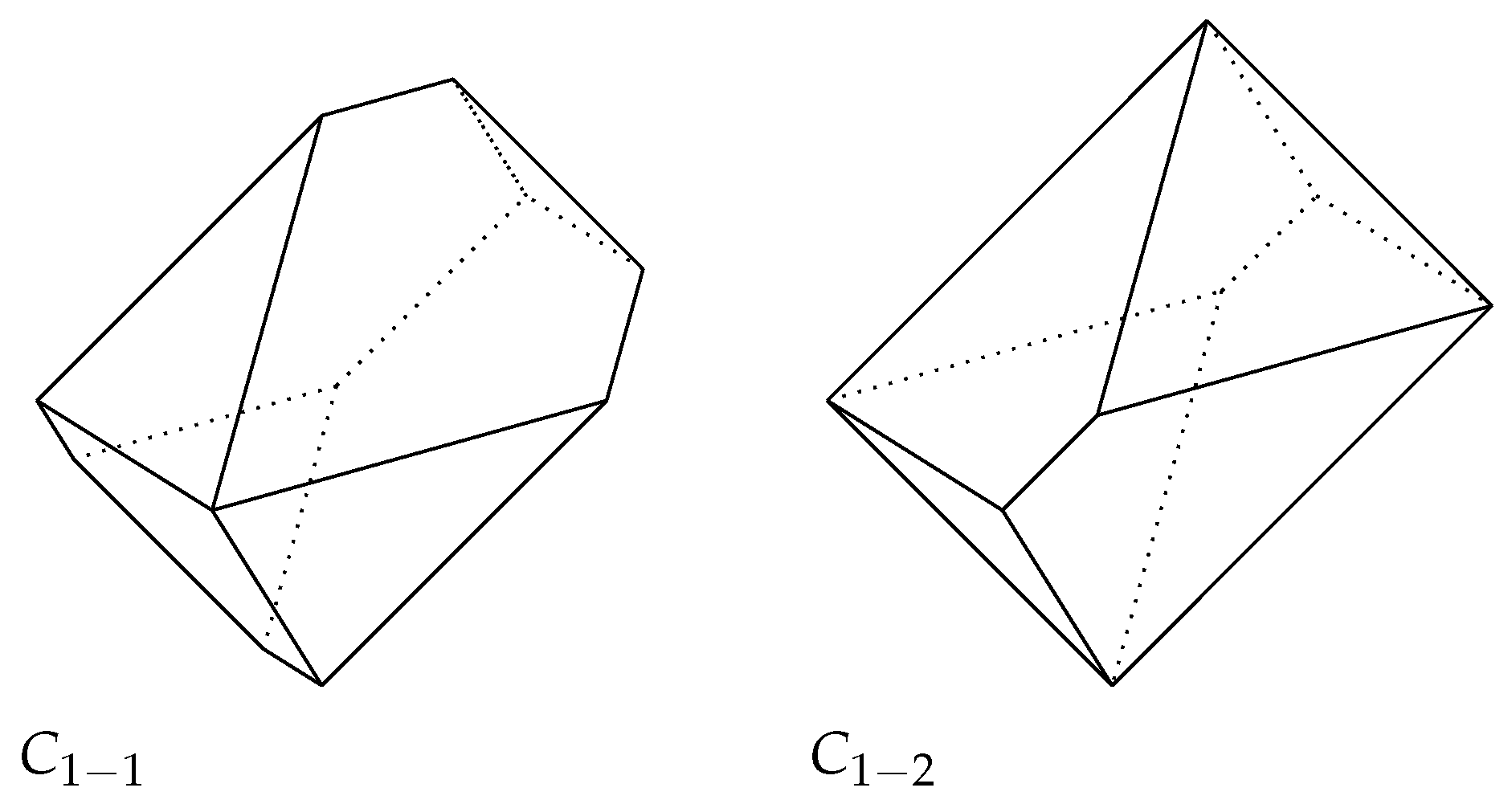
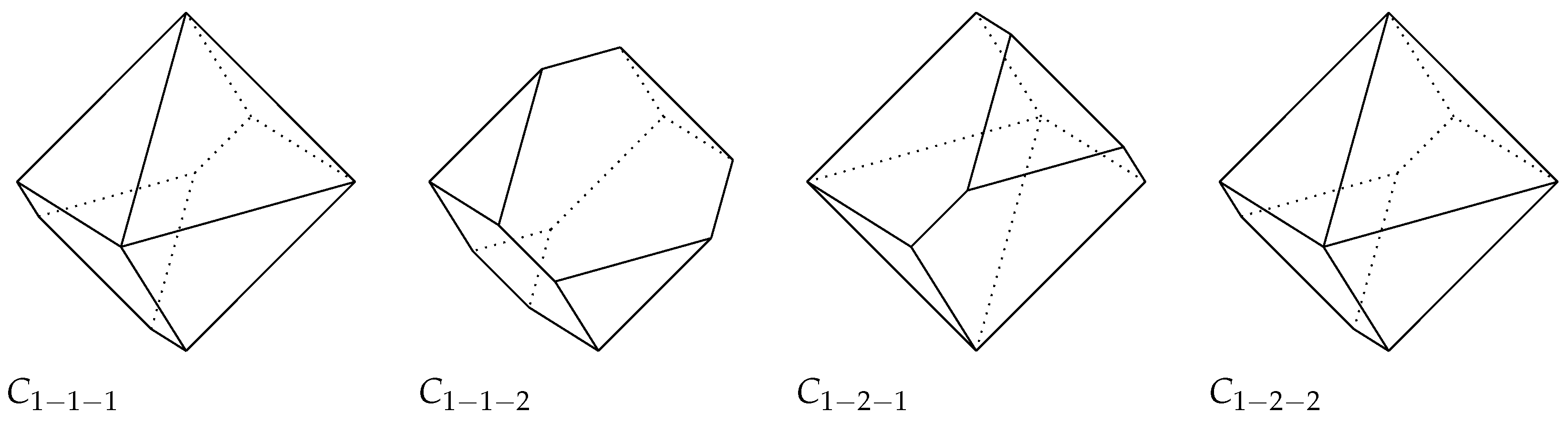
3. Borsuk’s Problem in ${\mathcal{\ell }}_{\mathbf{1}}^{\mathbf{3}}$

For each number $\alpha \in \mathbb{R}$, set

$$\sigma \left(\alpha \right)=\left\{\begin{array}{cc}1,\hfill & \alpha \ge 0,\hfill \\ -1,\hfill & \alpha <0.\hfill \end{array}\right.$$

Lemma 2.

Let $x=({\alpha }_1,\dots ,{\alpha }_n)$ be a unit vector in ${\mathcal{\ell }}_1^n$ and $f_x=(\sigma \left({\alpha }_1\right),\dots ,\sigma \left({\alpha }_n\right))\in {\mathcal{\ell }}_{\infty }^n$. Then, $f_x\in J\left(x\right)$.

Proof. 

Clearly, ${\Vert f_x\Vert }_{\infty }=1$ and $f_x\left(x\right)={\displaystyle \sum _{i\in \left[n\right]}}\left|{\alpha }_i\right|={\Vert x\Vert }_1={\Vert f_x\Vert }_{\infty }{\Vert x\Vert }_1$.    □

Let $Q_1,Q_2,Q_3,Q_4$ be the linear transforms with matrices

$$\left[\begin{array}{ccc}0& 0& -1\\ 0& -1& 0\\ -1& 0& 0\end{array}\right],\left[\begin{array}{ccc}-1& 0& 0\\ 0& 0& -1\\ 0& -1& 0\end{array}\right],\left[\begin{array}{ccc}0& 1& 0\\ 0& 0& 1\\ 1& 0& 0\end{array}\right],\left[\begin{array}{ccc}0& 0& -1\\ -1& 0& 0\\ 0& 1& 0\end{array}\right],$$

respectively. Set

$$u=({\displaystyle \frac{1}{3}},-{\displaystyle \frac{1}{3}},{\displaystyle \frac{1}{3}}),v=(-{\displaystyle \frac{1}{3}},{\displaystyle \frac{1}{3}},{\displaystyle \frac{1}{3}}),w=(-{\displaystyle \frac{1}{3}},-{\displaystyle \frac{1}{3}},{\displaystyle \frac{1}{3}}),\mathrm{and}p=({\displaystyle \frac{1}{3}},{\displaystyle \frac{1}{3}},{\displaystyle \frac{1}{3}}).$$

Clearly, ${\mathcal{C}}_0=\Vert B_1^3\Vert$ is a UCS for ${\mathcal{\ell }}_1^3$. By Lemma 2, $f_u=(1,-1,1)\in J\left(u\right)$. It is straightforward to check that

$$\begin{array}{c}a(u,-u)={\displaystyle \frac{1}{2}}u,b(u,-u)=-{\displaystyle \frac{1}{2}}u,\\ H_{f_u,b(u,-u)}^{+}=\left\{x\in {\mathcal{\ell }}_1^3|f_u\left(x\right)\ge -{\displaystyle \frac{1}{2}}\right\},\mathrm{and}{H}_{f_u,a(u,-u)}^{-}=\left\{x\in {\mathcal{\ell }}_1^3|f_u\left(x\right)\le {\displaystyle \frac{1}{2}}\right\}.\end{array}$$

Set $C_1=B_1^3(u,-u,f_u,+)$ and $C_2=B_1^3(u,-u,f_u,-)$. By Theorem 1, $\{C_1,C_2\}$ is also a UCS. The set of vertices of $C_1$ and $C_2$ can be calculated by the following SageMath code (see Listing 1):

Listing 1. Computing the vertices of $C_1$ and $C_2$.

# Generate an octahedron with vertices (±1, 0, 0), (0, ±1, 0), and (0, 0, ±1). C0 = polytopes.cross_polytope(3) #H1:$H_{f_u,b(u,-u)}^{+}=\left\{x\in {\mathcal{\ell }}_1^3|f_u\left(x\right)\ge -1/2\right\}.$ H1 = Polyhedron(ieqs=[(1/2, 1, −1, 1)]) #H2: $H_{f_u,a(u,-u)}^{-}=\left\{x\in {\mathcal{\ell }}_1^3|f_u\left(x\right)\le 1/2\right\}.$ H2 = Polyhedron(ieqs=[(1/2, −1, 1, −1)]) # Set C1 to be the intersection of C0 and H1. C1 = C0.intersection(H1) # Set C2 to be the intersection of C0 and H2. C2 = C0.intersection(H2) # Print the vertices of C1 and C2. print("Vertices of C1 are: {}. \nVertices of C2 are: {}".format(C1.vertices(), C2.vertices()))

We have (see Figure 1)

$$\begin{array}{cc}\hfill ext{C}_1=& \left\{(1,0,0),(0,-1,0),(0,0,1),\right.\hfill \\ & (-3/4,0,1/4),(0,3/4,1/4),(0,-1/4,-3/4),\hfill \\ & \left.(1/4,3/4,0),(1/4,0,-3/4),(-3/4,-1/4,0)\right\},\hfill \end{array}$$

and

$$\begin{array}{cc}\hfill ext{C}_2=& \left\{(0,0,-1),(0,1,0),(-1,0,0),\right.\hfill \\ \hfill & (-1/4,0,3/4),(-1/4,-3/4,0),(3/4,1/4,0),\hfill \\ \hfill & \left.(0,-3/4,-1/4),(3/4,0,-1/4),(0,1/4,3/4)\right\}.\hfill \end{array}$$

It can be seen that $C_1=Q_1\left(C_2\right)$, which implies that $C_2$ is an isometric copy of $C_1$. Hence, ${\mathcal{C}}_1=\left\{C_1\right\}$ is a UCS.

It can be verified by the code (see Listing 2):

Listing 2. Checking the containment.

# Check whether (−1/3, 1/3, 1/3) and (1/3, −1/3, −1/3) are both in C1. C1. contains ([−1/3, 1/3, 1/3]) and C1. contains ([1/3, −1/3, −1/3])

that $C_1$ contains both v and $-v$. As above, $f_v=(-1,1,1)\in J\left(v\right)$,

$$\begin{array}{c}a(v,-v)={\displaystyle \frac{1}{2}}v,b(v,-v)=-{\displaystyle \frac{1}{2}}v,\\ H_{f_v,b(v,-v)}^{+}=\left\{x\in {\mathcal{\ell }}_1^3|f_v\left(x\right)\ge -{\displaystyle \frac{1}{2}}\right\},\mathrm{and}{H}_{f_v,a(v,-v)}^{-}=\left\{x\in {\mathcal{\ell }}_1^3|f_v\left(x\right)\le {\displaystyle \frac{1}{2}}\right\}.\end{array}$$

Set $C_{1-1}=C_1(v,-v,f_v,+)$ and $C_{1-2}=C_1(v,-v,f_v,-)$. Straightforward calculations show that (see Figure 2)

$$\begin{array}{cc}\hfill ext{C}_{1-1}& =\left\{(0,-3/4,1/4),(0,0,1),(3/4,1/4,0),\right.\hfill \\ \hfill & (3/4,0,1/4),(-1/4,-3/4,0),(-1/4,-1/4,-1/2),\hfill \\ \hfill & (-3/4,-1/4,0),(1/4,3/4,0),(1/4,1/4,-1/2),\hfill \\ \hfill & \left.(-3/4,0,1/4),(0,3/4,1/4)\right\},\hfill \end{array}$$

and

$$\begin{array}{cc}\hfill ext{C}_{1-2}& =\left\{(-3/4,-1/4,0),(1/4,3/4,0),(1,0,0),\right.\hfill \\ \hfill & (1/4,0,3/4),(0,-1,0),(0,-1/4,3/4),\hfill \\ \hfill & \left.(0,-1/4,-3/4),(1/4,0,-3/4)\right\}.\hfill \end{array}$$

By Theorem 1, $\{C_{1-1},C_{1-2}\}$ is a UCS.

It can be verified that $C_{1-1}$ and $C_{1-2}$ contains both w and $-w$. As above, $f_w=(-1,-1,1)\in J\left(w\right)$,

$$\begin{array}{c}a(w,-w)={\displaystyle \frac{1}{2}}w,b(w,-w)=-{\displaystyle \frac{1}{2}}w,\\ H_{f_w,b(w,-w)}^{+}=\left\{x\in {\mathcal{\ell }}_1^3|f_w\left(x\right)\ge -{\displaystyle \frac{1}{2}}\right\},\mathrm{and}{H}_{f_w,a(w,-w)}^{-}=\left\{x\in {\mathcal{\ell }}_1^3|f_w\left(x\right)\le {\displaystyle \frac{1}{2}}\right\}.\end{array}$$

Set

$$\begin{array}{c}{C}_{1-1-1}=C_{1-1}(w,-w,f_w,+),C_{1-1-2}=C_{1-1}(w,-w,f_w,-),\\ C_{1-2-1}=C_{1-2}(w,-w,f_w,+),C_{1-2-2}=C_{1-2}(w,-w,f_w,-).\end{array}$$

By Theorem 1,

$$\{C_{1-1-1},C_{1-1-2},C_{1-2-1},C_{1-2-2}\}$$

is a UCS. Straightforward calculations show that (see Figure 3)

$$\begin{array}{cc}\hfill ext{C}_{1-1-1}& =\left\{(0,3/4,1/4),(0,0,1),(3/4,0,1/4),\right.\hfill \\ \hfill & (0,-3/4,1/4),(-1/4,-3/4,0),(-1/4,-1/4,-1/2),\hfill \\ \hfill & \left.(-3/4,-1/4,0),(0,0,-1/2),(-3/4,0,1/4)\right\},\hfill \\ \hfill ext{C}_{1-1-2}& =\left\{(0,3/4,1/4),(1/4,1/4,-1/2),(3/4,1/4,0),\right.\hfill \\ \hfill & (3/4,0,1/4),(1/4,3/4,0),(-1/4,-1/4,-1/2),\hfill \\ \hfill & (-1/4,-1/2,-1/4),(-1/2,-1/4,-1/4),(1/4,-1/2,1/4),\hfill \\ & \left.(1/4,0,3/4),(0,1/4,3/4),(-1/2,1/4,1/4)\right\},\hfill \\ \hfill ext{C}_{1-2-1}& =\left\{(0,-1/4,-3/4),(-3/4,-1/4,0),(3/4,-1/4,0),\right.\hfill \\ \hfill & (3/4,0,1/4),(1/4,1/2,1/4),(1/4,0,3/4),\hfill \\ \hfill & \left.(0,-1,0),(0,-1/4,3/4),(0,1/2,0)\right\},\hfill \\ \hfill ext{C}_{1-2-2}& =\left\{(1/4,0,3/4),(1/4,3/4,0),(1,0,0),\right.\hfill \\ \hfill & (0,-1/4,-3/4),(1/4,0,-3/4),(-1/2,-1/4,-1/4),\hfill \\ \hfill & \left.(0,-3/4,-1/4),(1/4,-3/4,0),(-1/2,0,0)\right\}.\hfill \end{array}$$

It can be seen that $C_{1-1-1}=Q_2\left(C_{1-2-1}\right)$ and $C_{1-1-1}=Q_3\left(C_{1-2-2}\right)$, which implies that $C_{1-2-1}$ and $C_{1-2-1}$ are isometric copies of $C_{1-1-1}$. Hence, ${\mathcal{C}}_3=\{C_{1-1-1},C_{1-1-2}\}$ is a UCS.

It can be verified that $C_{1-1-1}$ and $C_{1-1-2}$ contains both p and $-p$. As above, $f_p=(1,1,1)\in J\left(p\right)$,

$$\begin{array}{c}a(p,-p)={\displaystyle \frac{1}{2}}p,b(p,-p)=-{\displaystyle \frac{1}{2}}p,\\ H_{f_p,b(p,-p)}^{+}=\left\{x\in {\mathcal{\ell }}_1^3|f_p\left(x\right)\ge -{\displaystyle \frac{1}{2}}\right\},\mathrm{and}{H}_{f_p,a(p,-p)}^{-}=\left\{x\in {\mathcal{\ell }}_1^3|f_p\left(x\right)\le {\displaystyle \frac{1}{2}}\right\}.\end{array}$$

Set $C_{1-1-1-1}=C_{1-1-1}(p,-p,f_p,+)$ and $C_{1-1-1-2}=C_{1-1-1}(p,-p,f_p,-)$. $C_{1-1-2-1}=C_{1-1-2}(p,-p,f_p,+)$, and $C_{1-1-2-2}=C_{1-1-2}(p,-p,f_p,-)$. Straightforward calculations show that (see Figure 4)

$$\begin{array}{cc}\hfill ext{C}_{1-1-1-1}& =\left\{(-1/4,0,3/4),(-1/4,-3/4,0),(1/2,0,0),\right.\hfill \\ \hfill & (1/2,-1/4,1/4),(0,-3/4,1/4),(0,-1/4,3/4),\hfill \\ \hfill & (0,1/2,0),(0,0,-1/2),(-1/4,-1/4,-1/2),\hfill \\ \hfill & \left.(-3/4,-1/4,0),(-3/4,0,-1/4),(-1/4,1/2,1/4)\right\},\hfill \\ \hfill ext{C}_{1-1-1-2}& =\left\{(0,-3/4,1/4),(-3/4,0,1/4),(0,0,-1/2),\right.\hfill \\ \hfill & \left.(0,3/4,1/4),(0,0,1),(3/4,0,1/4)\right\},\hfill \\ \hfill ext{C}_{1-1-2-1}& =\left\{(-1/4,1/2,1/4),(1/4,1/4,-1/2),(1/2,-1/4,1/4),\right.\hfill \\ \hfill & (1/2,1/4,-1/4),(1/4,1/2,-1/4),(-1/4,-1/4,-1/2),\hfill \\ \hfill & (-1/2,-1/4,-1/4),(-1/4,-1/2,-1/4),(1/4,-1/4,1/2),\hfill \\ \hfill & \left.(1/4,-1/2,1/4),(-1/2,1/4,1/4),(-1/4,1/4,1/2)\right\}\hfill \\ \hfill ext{C}_{1-1-2-2}& =\left\{(0,3/4,1/4),(1/4,1/4,-1/2),(3/4,1/4,0),\right.\hfill \\ \hfill & (3/4,0,1/4),(1/4,3/4,0),(0,1/4,3/4),\hfill \\ \hfill & (-1/2,1/4,1/4),(1/4,-1/2,1/4),(1/4,0,3/4),\hfill \\ \hfill & \left.(0,-1/2,0),(-1/2,0,0),(0,0,-1/2)\right\}.\hfill \end{array}$$

It can be seen that $C_{1-1-1-1}=Q_4\left(C_{1-1-2-2}\right)$, which implies that $C_{1-1-1-1}$ is an isometric copy of $C_{1-1-2-2}$. Hence, ${\mathcal{C}}_4=\{C_{1-1-1-2},C_{1-1-2-1},C_{1-1-2-2}\}$ is a UCS.

In the rest of this paper, let

$$f_1=f_p,f_2=f_{-w},f_3=f_u\mathrm{and}{f}_4=f_v.$$

For each $K\in {\mathcal{K}}^3$ and $j\in \left[4\right]$, let $x_j\left(K\right),y_j\left(K\right)\in extK$ be two points such that

$$f_j\left(x_j\left(K\right)\right)=\underset{x\in K}{max}{f}_j\left(x\right)\mathrm{and}{f}_j\left(y_j\left(K\right)\right)=\underset{x\in K}{min}{f}_j\left(x\right).$$

Denote by $D_1$ the polytope $C_{1-1-2-2}$, $D_2$ the polytope $C_{1-1-1-2}$, and $D_3$ the polytope $C_{1-1-2-1}$. The foregoing discussion shows that ${\mathcal{D}}_0=D_1,D_2,D_3$ is a UCS. For each $D\in {\mathcal{D}}_0$, the points $x_1\left(D\right),y_1\left(D\right)$, $x_1\left(D\right)-y_1\left(D\right)$, $a(x_1\left(D\right),y_1\left(D\right))$, and $b(x_1\left(D\right),y_1\left(D\right))$ can be calculated by the code in [25]. The values corresponding to these variables are tabulated in

Table 1. The points $x_1\left(D\right),y_1\left(D\right)$, $x_1\left(D\right)-y_1\left(D\right)$, $a(x_1\left(D\right),y_1\left(D\right))$, $b(x_1\left(D\right),y_1\left(D\right))$ for $D\in {\mathcal{D}}_0$.

	${\mathit{x}}_1\left(\mathbf{·}\right)$	${\mathit{y}}_1\left(\mathbf{·}\right)$	${\mathit{x}}_1\left(\mathbf{·}\right)-{\mathit{y}}_1\left(\mathbf{·}\right)$	$\mathit{a}({\mathit{x}}_1\left(\mathbf{·}\right),{\mathit{y}}_1\left(\mathbf{·}\right))$	$\mathit{b}({\mathit{x}}_1\left(\mathbf{·}\right),{\mathit{y}}_1\left(\mathbf{·}\right))$
$D_1$	$(0,{\displaystyle \frac{1}{4}},{\displaystyle \frac{3}{4}})$	$(-{\displaystyle \frac{1}{2}},0,0)$	$({\displaystyle \frac{1}{2}},{\displaystyle \frac{1}{4}},{\displaystyle \frac{3}{4}})$	$(-{\displaystyle \frac{1}{12}},{\displaystyle \frac{5}{24}},{\displaystyle \frac{5}{8}})$	$(-{\displaystyle \frac{5}{12}},{\displaystyle \frac{1}{24}},{\displaystyle \frac{1}{8}})$
$D_2$	$(0,0,1)$	$(-{\displaystyle \frac{3}{4}},0,{\displaystyle \frac{1}{4}})$	$({\displaystyle \frac{3}{4}},0,{\displaystyle \frac{3}{4}})$	$(-{\displaystyle \frac{1}{8}},0,{\displaystyle \frac{7}{8}})$	$(-{\displaystyle \frac{5}{8}},0,{\displaystyle \frac{3}{8}})$
$D_3$	$(-{\displaystyle \frac{1}{4}},{\displaystyle \frac{1}{4}},{\displaystyle \frac{1}{2}})$	$(-{\displaystyle \frac{1}{2}},-{\displaystyle \frac{1}{4}},-{\displaystyle \frac{1}{4}})$	$({\displaystyle \frac{1}{4}},{\displaystyle \frac{1}{2}},{\displaystyle \frac{3}{4}})$	$(-{\displaystyle \frac{7}{24}},{\displaystyle \frac{1}{6}},{\displaystyle \frac{3}{8}})$	$(-{\displaystyle \frac{11}{24}},-{\displaystyle \frac{1}{6}},-{\displaystyle \frac{1}{8}})$

. Clearly, by Lemma 2,

$$f_1\in J\left({\displaystyle \frac{(x_1\left(D\right)-y_1\left(D\right))}{\Vert x_1\left(D\right)-y_1\left(D\right)\Vert }}\right).$$

From Theorem 1, it follows that

$$\left\{D_{i-1}:=D_i(x_1\left(D_i\right),y_1\left(D_i\right),f_1,-)|i\in \left[3\right]\right\}\cup \left\{D_{i-2}:=D_i(x_1\left(D_i\right),y_1\left(D_i\right),f_1,+)|i\in \left[3\right]\right\}$$

is a UCS for ${\mathcal{\ell }}_1^3$.

Given a polyhedron whose vertices are $v_1,\cdots ,v_n$, its centroid c is given by

$$c={\displaystyle \frac{{\sum }_{i=1}^n{v}_i}{n}}.$$

By Algorithm 2, we can obtain a reduced UCS

$${\mathcal{D}}_1=\{D_{1-1},D_{1-2},D_{2-1},D_{3-1},D_{3-2}\}.$$

Algorithm 2 Removing isometric copies from the members of a UCS

Input: A UCS $\mathcal{C}=\left\{C_i|i\in [k-1]\cup 0\right\}$; ${\mathcal{G}}_{{\mathcal{\ell }}_1^3}$.       1: Initialize $\mathcal{S}\leftarrow Ø$.       2: Initialize $\mathcal{U}\leftarrow Ø$.       3: for all  $C_i\in \mathcal{C}$do       4:       Compute the centroid $c_i$ of $C_i$.       5:       Set $C_i^{\prime }=C_i-c_i$.       6:       if $C_i^{\prime }\in \mathcal{S}$ then       7:             Continue       8:       end if       9:       $\mathcal{U}\leftarrow \mathcal{U}\cup \left\{C_i\right\}$     10:       $\mathcal{S}\leftarrow {\mathcal{G}}_{{\mathcal{\ell }}_1^3}\left(C_i^{\prime }\right)=\left\{T\left(C_i^{\prime }\right)|T\in {\mathcal{G}}_{{\mathcal{\ell }}_1^3}\right\}$     11: end for     12: return  $\mathcal{U}$

For each $D\in {\mathcal{D}}_1$, see

Table 2. The points $x_2\left(D\right)$, $y_2\left(D\right)$, $x_2\left(D\right)-y_2\left(D\right)$, $a(x_2\left(D\right),y_2\left(D\right))$, $b(x_2\left(D\right),y_2\left(D\right))$ for $D\in {\mathcal{D}}_1$.

	${\mathit{x}}_2\left(\mathbf{·}\right)$	${\mathit{y}}_2\left(\mathbf{·}\right)$	${\mathit{x}}_2\left(\mathbf{·}\right)-{\mathit{y}}_2\left(\mathbf{·}\right)$	$\mathit{a}({\mathit{x}}_2\left(\mathbf{·}\right),{\mathit{y}}_2\left(\mathbf{·}\right))$	$\mathit{b}({\mathit{x}}_2\left(\mathbf{·}\right),{\mathit{y}}_2\left(\mathbf{·}\right))$
$D_{1-1}$	$({\displaystyle \frac{1}{4}},{\displaystyle \frac{5}{8}},-{\displaystyle \frac{1}{8}})$	$({\displaystyle \frac{1}{4}},-{\displaystyle \frac{1}{8}},{\displaystyle \frac{5}{8}})$	$(0,{\displaystyle \frac{3}{4}},-{\displaystyle \frac{3}{4}})$	$({\displaystyle \frac{1}{4}},{\displaystyle \frac{1}{2}},0)$	$({\displaystyle \frac{1}{4}},0,{\displaystyle \frac{1}{2}})$
$D_{1-2}$	$({\displaystyle \frac{1}{4}},{\displaystyle \frac{3}{4}},0)$	$({\displaystyle \frac{1}{4}},0,{\displaystyle \frac{3}{4}})$	$(0,{\displaystyle \frac{3}{4}},-{\displaystyle \frac{3}{4}})$	$({\displaystyle \frac{1}{4}},{\displaystyle \frac{5}{8}},{\displaystyle \frac{1}{8}})$	$({\displaystyle \frac{1}{4}},{\displaystyle \frac{1}{8}},{\displaystyle \frac{5}{8}})$
$D_{2-1}$	$(0,0,-{\displaystyle \frac{1}{2}})$	$(0,-{\displaystyle \frac{3}{4}},{\displaystyle \frac{1}{4}})$	$(0,{\displaystyle \frac{3}{4}},-{\displaystyle \frac{3}{4}})$	$(0,-{\displaystyle \frac{1}{8}},-{\displaystyle \frac{3}{8}})$	$(0,-{\displaystyle \frac{5}{8}},{\displaystyle \frac{1}{8}})$
$D_{3-1}$	$({\displaystyle \frac{1}{4}},{\displaystyle \frac{1}{4}},-{\displaystyle \frac{1}{2}})$	$(-{\displaystyle \frac{1}{2}},-{\displaystyle \frac{1}{4}},-{\displaystyle \frac{1}{4}})$	$({\displaystyle \frac{3}{4}},{\displaystyle \frac{1}{2}}-{\displaystyle \frac{1}{4}})$	$({\displaystyle \frac{1}{8}},{\displaystyle \frac{1}{6}},-{\displaystyle \frac{11}{24}})$	$(-{\displaystyle \frac{3}{8}},-{\displaystyle \frac{1}{6}},-{\displaystyle \frac{7}{24}})$
$D_{3-2}$	$({\displaystyle \frac{1}{4}},{\displaystyle \frac{1}{4}},-{\displaystyle \frac{1}{2}})$	$(-{\displaystyle \frac{1}{4}},{\displaystyle \frac{1}{4}},{\displaystyle \frac{1}{2}})$	$({\displaystyle \frac{1}{2}},0,-1)$	$({\displaystyle \frac{1}{6}},{\displaystyle \frac{1}{4}},-{\displaystyle \frac{1}{3}})$	$(-{\displaystyle \frac{1}{6}},{\displaystyle \frac{1}{4}},{\displaystyle \frac{1}{3}})$

(see [25]) for the coordinates of $x_2\left(D\right),y_2\left(D\right)$, $x_2\left(D\right)-y_2\left(D\right)$, $a(x_2\left(D\right),y_2\left(D\right))$, $b(x_2\left(D\right),y_2\left(D\right))$, resp.

By Lemma 2,

$$f_2\in J\left({\displaystyle \frac{(x_2\left(D\right)-y_2\left(D\right))}{\Vert x_2\left(D\right)-y_2\left(D\right)\Vert }}\right),\forall D\in {\mathcal{D}}_1.$$

For each $i\in \left[3\right]$, set

$$\begin{array}{cc}\hfill & D_{i-1-1}=D_{i-1}(x_2\left(D_{i-1}\right),y_2\left(D_{i-1}\right),f_2,-),D_{i-1-2}=D_{i-1}(x_2\left(D_{i-1}\right),y_2\left(D_{i-1}\right),f_2,+),\hfill \\ \hfill & D_{i-2-1}=D_{i-2}(x_2\left(D_{i-2}\right),y_2\left(D_{i-2}\right),f_2,-),D_{i-2-2}=D_{i-2}(x_2\left(D_{i-2}\right),y_2\left(D_{i-2}\right),f_2,+).\hfill \end{array}$$

By applying Theorem 1 and Algorithm 2, a reduced UCS

$${\mathcal{D}}_2=\{D_{1-1-1},D_{1-1-2},D_{1-2-1},D_{2-1-1},D_{3-1-1},D_{3-1-2}\}$$

can be generated from ${\mathcal{D}}_1$.

For each $D\in {\mathcal{D}}_2$, see

Table 3. The points $x_3\left(D\right),y_3\left(D\right)$, $x_3\left(D\right)-y_3\left(D\right)$, $a(x_3\left(D\right),y_3\left(D\right))$, $b(x_3\left(D\right),y_3\left(D\right))$ for $D\in {\mathcal{D}}_2$.

	${\mathit{x}}_3\left(\mathbf{·}\right)$	${\mathit{y}}_3\left(\mathbf{·}\right)$	${\mathit{x}}_3\left(\mathbf{·}\right)-{\mathit{y}}_3\left(\mathbf{·}\right)$	$\mathit{a}({\mathit{x}}_3\left(\mathbf{·}\right),{\mathit{y}}_3\left(\mathbf{·}\right))$	$\mathit{b}({\mathit{x}}_3\left(\mathbf{·}\right),{\mathit{y}}_3\left(\mathbf{·}\right))$
$D_{1-1-1}$	$({\displaystyle \frac{5}{8}},-{\displaystyle \frac{1}{8}},{\displaystyle \frac{1}{4}})$	$(-{\displaystyle \frac{1}{8}},{\displaystyle \frac{5}{8}},{\displaystyle \frac{1}{4}})$	$({\displaystyle \frac{3}{4}},-{\displaystyle \frac{3}{4}},0)$	$({\displaystyle \frac{1}{2}},0,{\displaystyle \frac{1}{4}})$	$(0,{\displaystyle \frac{1}{2}},{\displaystyle \frac{1}{4}})$
$D_{1-1-2}$	$({\displaystyle \frac{5}{8}},-{\displaystyle \frac{1}{8}},{\displaystyle \frac{1}{4}})$	$(-{\displaystyle \frac{1}{8}},{\displaystyle \frac{5}{8}},{\displaystyle \frac{1}{4}})$	$({\displaystyle \frac{3}{4}},-{\displaystyle \frac{3}{4}},0)$	$({\displaystyle \frac{1}{2}},0,{\displaystyle \frac{1}{4}})$	$(0,{\displaystyle \frac{1}{2}},{\displaystyle \frac{1}{4}})$
$D_{1-2-1}$	$({\displaystyle \frac{3}{4}},0,{\displaystyle \frac{1}{4}})$	$({\displaystyle \frac{1}{8}},{\displaystyle \frac{1}{8}},-{\displaystyle \frac{1}{2}})$	$({\displaystyle \frac{5}{8}},-{\displaystyle \frac{1}{8}},{\displaystyle \frac{3}{4}})$	$({\displaystyle \frac{31}{48}},{\displaystyle \frac{1}{48}},{\displaystyle \frac{1}{8}})$	$({\displaystyle \frac{11}{48}},{\displaystyle \frac{5}{48}},-{\displaystyle \frac{3}{8}})$
$D_{2-1-1}$	$(0,-{\displaystyle \frac{3}{4}},{\displaystyle \frac{1}{4}})$	$(-{\displaystyle \frac{3}{4}},0,{\displaystyle \frac{1}{4}})$	$({\displaystyle \frac{3}{4}},-{\displaystyle \frac{3}{4}},0)$	$(-{\displaystyle \frac{1}{8}},-{\displaystyle \frac{5}{8}},{\displaystyle \frac{1}{4}})$	$(-{\displaystyle \frac{5}{8}},-{\displaystyle \frac{1}{8}},{\displaystyle \frac{1}{4}})$
$D_{3-1-1}$	$({\displaystyle \frac{3}{8}},-{\displaystyle \frac{3}{8}},{\displaystyle \frac{1}{4}})$	$(-{\displaystyle \frac{3}{8}},{\displaystyle \frac{3}{8}},{\displaystyle \frac{1}{4}})$	$({\displaystyle \frac{3}{4}},-{\displaystyle \frac{3}{4}},0)$	$({\displaystyle \frac{1}{4}},-{\displaystyle \frac{1}{4}},{\displaystyle \frac{1}{4}})$	$(-{\displaystyle \frac{1}{4}},{\displaystyle \frac{1}{4}},{\displaystyle \frac{1}{4}})$
$D_{3-1-2}$	$({\displaystyle \frac{3}{8}},-{\displaystyle \frac{3}{8}},{\displaystyle \frac{1}{4}})$	$(-{\displaystyle \frac{3}{8}},{\displaystyle \frac{3}{8}},{\displaystyle \frac{1}{4}})$	$({\displaystyle \frac{3}{4}},-{\displaystyle \frac{3}{4}},0)$	$({\displaystyle \frac{1}{4}},-{\displaystyle \frac{1}{4}},{\displaystyle \frac{1}{4}})$	$(-{\displaystyle \frac{1}{4}},{\displaystyle \frac{1}{4}},{\displaystyle \frac{1}{4}})$

(see [25]) for the coordinates of $x_3\left(D\right),y_3\left(D\right)$, $x_3\left(D\right)-y_3\left(D\right)$, $a(x_3\left(D\right),y_3\left(D\right))$, $b(x_3\left(D\right),y_3\left(D\right))$, resp.

By Lemma 2,

$$f_3\in J\left({\displaystyle \frac{(x_3\left(D\right)-y_3\left(D\right))}{\Vert x_3\left(D\right)-y_3\left(D\right)\Vert }}\right),\forall D\in {\mathcal{D}}_2.$$

For each $i\in \left[3\right]$, set

$$\begin{array}{cc}\hfill D_{i-1-1-1}& =D_{i-1-1}(x_3\left(D_{i-1-1}\right),y_3\left(D_{i-1-1}\right),f_3,-),\hfill \\ \hfill D_{i-1-1-2}& =D_{i-1-1}(x_3\left(D_{i-1-1}\right),y_3\left(D_{i-1-1}\right),f_3,+),\hfill \\ \hfill D_{i-1-2-1}& =D_{i-1-2}(x_3\left(D_{i-1-2}\right),y_3\left(D_{i-1-2}\right),f_3,-),\hfill \\ \hfill D_{i-1-2-2}& =D_{i-1-2}(x_3\left(D_{i-1-2}\right),y_3\left(D_{i-1-2}\right),f_3,+),\hfill \\ \hfill D_{i-2-1-1}& =D_{i-2-1}(x_3\left(D_{i-2-1}\right),y_3\left(D_{i-2-1}\right),f_3,-),\hfill \\ \hfill D_{i-2-1-2}& =D_{i-2-1}(x_3\left(D_{i-2-1}\right),y_3\left(D_{i-2-1}\right),f_3,+).\hfill \end{array}$$

By applying Theorem 1 and Algorithm 2, a reduced UCS

$${\mathcal{D}}_3=\{D_{1-1-1-1},D_{1-1-1-2},D_{1-1-2-2},D_{1-2-1-1},D_{3-1-1-2},D_{3-1-2-2}\}$$

can be generated from ${\mathcal{D}}_2$.

For each $D\in {\mathcal{D}}_3$, see

Table 4. The points $x_4\left(D\right),y_4\left(D\right)$, $x_4\left(D\right)-y_4\left(D\right)$, $a(x_4\left(D\right),y_4\left(D\right))$, $b(x_4\left(D\right),y_4\left(D\right))$ for $D\in {\mathcal{D}}_3$.

	${\mathit{x}}_4\left(\mathbf{·}\right)$	${\mathit{y}}_4\left(\mathbf{·}\right)$	${\mathit{x}}_4\left(\mathbf{·}\right)-{\mathit{y}}_4\left(\mathbf{·}\right)$	$\mathit{a}({\mathit{x}}_4\left(\mathbf{·}\right),{\mathit{y}}_4\left(\mathbf{·}\right))$	$\mathit{b}({\mathit{x}}_4\left(\mathbf{·}\right),{\mathit{y}}_4\left(\mathbf{·}\right))$
$D_{1-1-1-1}$	$(-\frac{1}{8},\frac{5}{8},\frac{1}{4})$	$(\frac{5}{8},0,\frac{1}{8})$	$(-\frac{3}{4},\frac{5}{8},\frac{1}{8})$	$(0,\frac{25}{48},\frac{11}{48})$	$(\frac{1}{2},\frac{5}{48},\frac{7}{48})$
$D_{1-1-1-2}$	$(-\frac{1}{8},\frac{1}{4},\frac{5}{8})$	$(0,-\frac{1}{2},0)$	$(-\frac{1}{8},\frac{3}{4},\frac{5}{8})$	$(-\frac{5}{48},\frac{1}{8},\frac{25}{48})$	$(-\frac{1}{48},-\frac{3}{8},\frac{5}{48})$
$D_{1-1-2-2}$	$(-\frac{1}{8},\frac{1}{2},\frac{3}{8})$	$(0,-\frac{1}{8},-\frac{3}{8})$	$(-\frac{1}{8},\frac{5}{8},\frac{3}{4})$	$(-\frac{5}{48},\frac{19}{48},\frac{1}{4})$	$(-\frac{1}{48},-\frac{1}{48},-\frac{1}{4})$
$D_{1-2-1-1}$	$(0,\frac{3}{4},\frac{1}{4})$	$(\frac{1}{8},\frac{1}{8},-\frac{1}{2})$	$(-\frac{1}{8},\frac{5}{8},\frac{3}{4})$	$(\frac{1}{48},\frac{31}{48},\frac{1}{8})$	$(\frac{5}{48},\frac{11}{48},-\frac{3}{8})$
$D_{3-1-1-2}$	$(-\frac{3}{8},\frac{1}{4},\frac{3}{8})$	$(\frac{1}{4},-\frac{1}{2},\frac{1}{4})$	$(-\frac{5}{8},\frac{3}{4},\frac{1}{8})$	$(-\frac{13}{48},\frac{1}{8},\frac{17}{48})$	$(\frac{7}{48},-\frac{3}{8},\frac{13}{48})$
$D_{3-1-2-2}$	$(-\frac{1}{4},\frac{1}{4},\frac{1}{4})$	$(-\frac{1}{4},-\frac{3}{8},-\frac{3}{8})$	$(0,\frac{5}{8},\frac{5}{8})$	$(-\frac{1}{4},\frac{3}{16},\frac{3}{16})$	$(-\frac{1}{4},-\frac{5}{16},-\frac{5}{16})$

(see [25]) for the coordinates of $x_4\left(D\right),y_4\left(D\right)$, $x_4\left(D\right)-y_4\left(D\right)$, $a(x_4\left(D\right),y_4\left(D\right))$, $b(x_4\left(D\right),y_4\left(D\right))$, resp.

By Lemma 2,

$$f_4\in J\left({\displaystyle \frac{(x_4\left(D\right)-y_4\left(D\right))}{\Vert x_4\left(D\right)-y_4\left(D\right)\Vert }}\right),\forall D\in {\mathcal{D}}_3.$$

For each $i\in \left[3\right]$, set

$$\begin{array}{cc}\hfill D_{i-1-1-1-1}& =D_{i-1-1-1}(x_3\left(D_{i-1-1-1}\right),y_3\left(D_{i-1-1-1}\right),f_3,-),\hfill \\ \hfill D_{i-1-1-1-2}& =D_{i-1-1-1}(x_3\left(D_{i-1-1-1}\right),y_3\left(D_{i-1-1-1}\right),f_3,+),\hfill \\ \hfill D_{i-1-1-2-1}& =D_{i-1-1-2}(x_3\left(D_{i-1-1-2}\right),y_3\left(D_{i-1-1-2}\right),f_3,-),\hfill \\ \hfill D_{i-1-1-2-2}& =D_{i-1-1-2}(x_3\left(D_{i-1-1-2}\right),y_3\left(D_{i-1-1-2}\right),f_3,+),\hfill \\ \hfill D_{i-1-2-2-1}& =D_{i-1-2-2}(x_3\left(D_{i-1-2-2}\right),y_3\left(D_{i-1-2-2}\right),f_3,-),\hfill \\ \hfill D_{i-1-2-2-2}& =D_{i-1-2-2}(x_3\left(D_{i-1-2-2}\right),y_3\left(D_{i-1-2-2}\right),f_3,+),\hfill \\ \hfill D_{i-2-1-1-1}& =D_{i-2-1-1}(x_3\left(D_{i-2-1-1}\right),y_3\left(D_{i-2-1-1}\right),f_3,-),\hfill \\ \hfill D_{i-2-1-1-2}& =D_{i-2-1-1}(x_3\left(D_{i-2-1-1}\right),y_3\left(D_{i-2-1-1}\right),f_3,+).\hfill \end{array}$$

Set $E_1=D_{1-1-1-1-1}$, $E_2=D_{1-1-1-1-2}$, $E_3=D_{1-1-1-2-2}$, $E_4=D_{1-1-2-2-2}$, $E_5=D_{1-2-1-1-1}$, $E_6=D_{3-1-1-2-2}$, $E_7=D_{3-1-2-2-1}$, $E_8=D_{3-1-2-2-2}$. By Theorem 1 and Algorithm 2, a reduced UCS (see Figure 5)

$$\mathcal{E}=\left\{E_i|i\in \left[8\right]\right\}$$

can be generated from ${\mathcal{D}}_3$.

We have

$$\begin{array}{cc}\hfill ext{E}_1& =\left\{\left(-1/2,0,0\right),\left(-1/2,1/8,1/8\right),\left(0,-1/2,0\right),\right.\hfill \\ \hfill & \left(0,0,-1/2\right),\left(0,1/8,5/8\right),\left(0,5/8,1/8\right),\hfill \\ \hfill & \left(1/8,-1/2,1/8\right),\left(1/8,0,5/8\right),\left(1/8,1/8,-1/2\right),\hfill \\ \hfill & \left(1/8,5/8,0\right),\left(5/8,0,1/8\right),\left(5/8,1/8,0\right)\};\hfill \end{array}$$

$$\begin{array}{cc}\hfill ext{E}_2& =\left\{\left(-1/2,0,0\right),\left(-1/2,1/4,1/4\right),\left(-1/8,-3/8,0\right),\right.\hfill \\ \hfill & \left(-1/8,0,-3/8\right),\left(-1/8,1/4,5/8\right),\left(-1/8,5/8,1/4\right),\hfill \\ \hfill & \left(1/8,-3/8,1/4\right),\left(1/8,0,5/8\right),\left(1/8,1/4,-3/8\right),\hfill \\ \hfill & \left(1/8,5/8,0\right),\left(1/2,0,1/4\right),\left(1/2,1/4,0\right)\};\hfill \end{array}$$

$$\begin{array}{cc}\hfill ext{E}_3& =\left\{\left(-3/8,-1/8,0\right),\left(-3/8,1/4,3/8\right),\left(-1/8,-3/8,0\right),\right.\hfill \\ \hfill & \left(-1/8,-1/8,-1/4\right),\left(-1/8,1/4,5/8\right),\left(-1/8,1/2,3/8\right),\hfill \\ \hfill & \left(1/4,-3/8,3/8\right),\left(1/4,-1/8,5/8\right),\left(1/4,1/4,-1/4\right),\hfill \\ \hfill & \left(1/4,1/2,0\right),\left(1/2,-1/8,3/8\right),\left(1/2,1/4,0\right)\};\hfill \end{array}$$

$$\begin{array}{cc}\hfill ext{E}_4& =\left\{\left(-1/4,-1/8,-1/8\right),\left(-1/4,3/8,3/8\right),\left(-1/8,-1/4,-1/8\right),\right.\hfill \\ \hfill & \left(-1/8,-1/8,-1/4\right),\left(-1/8,3/8,1/2\right),\left(-1/8,1/2,3/8\right),\hfill \\ \hfill & \left(3/8,-1/4,3/8\right),\left(3/8,-1/8,1/2\right),\left(3/8,3/8,-1/4\right),\hfill \\ \hfill & \left(3/8,1/2,-1/8\right),\left(1/2,-1/8,3/8\right),\left(1/2,3/8,-1/8\right)\};\hfill \end{array}$$

$$\begin{array}{cc}\hfill ext{E}_5& =\left\{\left(-1/2,1/8,1/8\right),\left(1/8,-1/2,1/8\right),\left(1/8,1/8,-1/2\right),\right.\hfill \\ \hfill & \left(1/8,1/8,3/4\right),\left(1/8,3/4,1/8\right),\left(3/4,1/8,1/8\right)\};\hfill \end{array}$$

$$\begin{array}{cc}\hfill ext{E}_6& =\left\{\left(-3/8,-3/8,-1/4\right),\left(-3/8,1/4,3/8\right),\left(1/4,-3/8,3/8\right),\right.\hfill \\ \hfill & \left(1/4,1/4,-1/4\right)\};\hfill \end{array}$$

$$\begin{array}{cc}\hfill ext{E}_7& =\left\{\left(3/8,1/4,-3/8\right),\left(3/8,-3/8,1/4\right),\left(-1/4,-3/8,-3/8\right),\right.\hfill \\ \hfill & \left(-1/4,3/16,3/16\right),\left(-3/16,1/4,3/16\right),\left(-3/16,3/16,1/4\right);\hfill \end{array}$$

$$\begin{array}{cc}\hfill ext{E}_8& =\left\{\left(5/16,1/4,-5/16\right),\left(5/16,-5/16,1/4\right),\left(-1/4,1/4,1/4\right),\right.\hfill \\ \hfill & \left(-1/4,-5/16,-5/16\right)\}.\hfill \end{array}$$

4. An Estimation of $\mathit{\beta }({\mathcal{\ell }}_{\mathbf{1}}^{\mathbf{3}},\mathbf{8})$

Proposition 4.

$E_1\subseteq {\displaystyle \frac{11}{16}}{B}_1^3+({\displaystyle \frac{1}{16}},{\displaystyle \frac{1}{16}},{\displaystyle \frac{1}{16}})$.

Proof. 

The desired inclusion follows directly from

$${\Vert e-({\displaystyle \frac{1}{16}},{\displaystyle \frac{1}{16}},{\displaystyle \frac{1}{16}})\Vert }_1\le {\displaystyle \frac{11}{16}},\forall e\in ext{E}_1.\square$$

Theorem 3.

${\tilde{\beta }}_{{\mathcal{\ell }}_1^3}(E_1,8)\le {\displaystyle \frac{11}{12}}$, ${\tilde{\beta }}_{{\mathcal{\ell }}_1^3}(E_5,8)\le {\displaystyle \frac{5}{6}}$.

Proof. 

By Proposition 4, $E_1$ can be covered by a ball centered at $(1/16,1/16,1/16)$ whose radius is $11/16$. Since the unit ball of ${\mathcal{\ell }}_1^3$ can be covered by eight balls having radius $2/3$ (cf. [26]), $E_1$ can be partitioned into eight subsets with diameters $11/12$. Since $E_5$ is a ball with a diameter $5/4$, $E_5$ can be partitioned into eight subsets with diameters $5/6$.    □

Proposition 5.

Let $B=24E_2-(0,3,3)$ (see Figure 6) be the polyhedron in ${\mathcal{\ell }}_1^3$ with vertices

$$\begin{array}{cccccccc}\hfill a_1& =(-12,3,3),\hfill & \hfill a_2& =(-3,-12,-3),\hfill & \hfill a_3& =(-3,-3,-12),\hfill & \hfill a_4& =(-12,-3,-3),\hfill \\ \hfill a_5& =(-3,3,12),\hfill & \hfill a_6& =(-3,12,3),\hfill & \hfill a_7& =(3,-12,3),\hfill & \hfill a_8& =(3,-3,12),\hfill \\ \hfill a_9& =(3,3,-12),\hfill & \hfill a_{10}& =(3,12,-3),\hfill & \hfill a_{11}& =(12,-3,3),\hfill & \hfill a_{12}& =(12,3,-3).\hfill \end{array}$$

Then, B can be partitioned into eight sets whose diameters are not greater than 22.

Proof. 

Set

$$\begin{array}{cccccccc}\hfill c_1& =({\displaystyle \frac{3}{2}},-{\displaystyle \frac{3}{2}},4),\hfill & \hfill c_2& =(-{\displaystyle \frac{3}{2}},{\displaystyle \frac{3}{2}},4),\hfill & \hfill c_3& =(7,0,0),\hfill & \hfill c_4& =(0,7,0),\hfill \\ \hfill c_5& =(-7,0,0),\hfill & \hfill c_6& =(0,-7,0),\hfill & \hfill c_7& =(-{\displaystyle \frac{3}{2}},-{\displaystyle \frac{3}{2}},-4),\hfill & \hfill c_8& =({\displaystyle \frac{3}{2}},{\displaystyle \frac{3}{2}},-4).\hfill \end{array}$$

We show that

$$B\subseteq \bigcup _{i\in \left[8\right]}(11B_1^3+c_i).$$

One can verify that $(0,0,0)$ is the centroid of B. Since ${\Vert (0,0,0)-c_i\Vert }_1\le 11,\forall i\in \left[8\right]$, we only need to prove that $bdB\subseteq {\bigcup }_{i\in \left[8\right]}(11B_1^3+c_i)$.

Let

$$Q_5=\left[\begin{array}{ccc}0& -1& 0\\ -1& 0& 0\\ 0& 0& 1\end{array}\right]\mathrm{and}{Q}_6=\left[\begin{array}{ccc}0& 1& 0\\ 1& 0& 0\\ 0& 0& 1\end{array}\right].$$

It can be seen that

$$\begin{array}{c}conv\left\{a_1,a_5,a_6\right\}=Q_6(conv\{a_7,a_8,a_{11}\left\}\right),c_i=Q_6\left(c_j\right),\forall i\in \{2,4,5\},j\in \{1,3,6\},\\ conv\left\{a_9,a_{10},a_{12}\right\}=Q_5(conv\{a_3,a_4,a_2\left\}\right),c_i=Q_5\left(c_j\right),\forall i\in \{3,4,8\},j\in \{5,6,7\},\\ conv\left\{a_5,a_6,a_8,a_{10},a_{11},a_{12}\right\}=Q_5(conv\{a_5,a_1,a_8,a_4,a_7,a_2\left\}\right),\\ c_i=Q_5\left(c_j\right),\forall i\in \{1,2,3,4\},j\in \{1,2,5,6\},\\ conv\left\{a_1,a_3,a_4,a_6,a_9,a_{10}\right\}=Q_6(conv\{a_7,a_3,a_2,a_{11},a_9,a_{12}\left\}\right),\\ c_i=Q_6\left(c_j\right)\forall i\in \{4,5,7,8\},j\in \{3,6,7,8\}.\end{array}$$

Thus, we only need to show that

$$\bigcup _{i\in \left[4\right]}{F}_i\subseteq (11B_1^3+c_j),\forall j\in \left[8\right],$$

where

$$\begin{array}{c}{F}_1=conv\{a_1,a_5,a_6\},F_2=conv\{a_9,a_{10},a_{12}\},\\ F_3=conv\{a_5,a_6,a_8,a_{10},a_{11},a_{12}\},\mathrm{and}{F}_4=conv\{a_1,a_3,a_4,a_6,a_9,a_{10}\}.\end{array}$$

For $F_1$ (see Figure 7), take

$$\begin{array}{c}{d}_1={\displaystyle \frac{5}{9}}{a}_5+{\displaystyle \frac{4}{9}}{a}_6=(-3,7,8),d_2={\displaystyle \frac{4}{9}}{a}_1+{\displaystyle \frac{5}{9}}{a}_5=(-7,3,8),\\ d_3={\displaystyle \frac{4}{9}}{a}_1+{\displaystyle \frac{1}{9}}{a}_5+{\displaystyle \frac{4}{9}}{a}_6=(-7,7,4),\mathrm{and}{d}_4={\displaystyle \frac{4}{9}}{a}_1+{\displaystyle \frac{5}{9}}{a}_6=(-7,8,3).\end{array}$$

We have

$$\begin{array}{cc}\hfill F_1=conv\{a_6,d_1,d_3,d_4\}& \cup conv\{a_1,d_2,d_4\}\cup conv\{a_5,d_1,d_2,d_3\},\hfill \\ \hfill {\Vert x-c_4\Vert }_1& \le 11,\forall x\in \{a_6,d_1,d_3,d_4\},\hfill \\ \hfill {\Vert x-c_5\Vert }_1& \le 11,\forall x\in \{a_1,d_2,d_4\},\hfill \\ \hfill {\Vert x-c_2\Vert }_1& \le 11,\forall x\in \{a_5,d_1,d_2,d_3\}.\hfill \end{array}$$

It follows that

$$F_1\subseteq \bigcup _{i\in \{2,4,5\}}(11B_1^3+c_i).$$

For $F_2$ (see Figure 8), take

$$\begin{array}{c}{e}_1={\displaystyle \frac{5}{9}}{a}_9+{\displaystyle \frac{4}{9}}{a}_{12}=(7,3,-8),e_2={\displaystyle \frac{5}{9}}{a}_9+{\displaystyle \frac{4}{9}}{a}_{10}=(3,7,-8),\\ e_3={\displaystyle \frac{1}{9}}{a}_9+{\displaystyle \frac{4}{9}}{a}_{10}+{\displaystyle \frac{4}{9}}{a}_{12}=(7,7,-4),\mathrm{and}{e}_4={\displaystyle \frac{5}{9}}{a}_{10}+{\displaystyle \frac{4}{9}}{a}_{12}=(7,8,-3).\end{array}$$

We have

$$\begin{array}{c}{F}_2=conv\{a_{12},e_1,e_4\}\cup conv\{a_{10},e_2,e_3,e_4\}\cup conv\{a_9,e_1,e_2,e_3\},\\ {\Vert x-c_3\Vert }_1\le 11,\forall x\in \{a_{12},e_1,e_4\},\\ {\Vert x-c_4\Vert }_1\le 11,\forall x\in \{a_{10},e_2,e_3,e_4\},\\ {\Vert x-c_8\Vert }_1\le 11,\forall x\in \{a_9,e_1,e_2,e_3\}.\end{array}$$

It follows that

$$F_2\subseteq \bigcup _{i\in \{3,4,8\}}(11B_1^3+c_i).$$

For $F_3$ (see Figure 9), take

$$\begin{array}{c}{m}_1={\displaystyle \frac{1}{2}}{a}_5+{\displaystyle \frac{1}{2}}{a}_8=(0,0,12),m_2={\displaystyle \frac{1}{9}}{a}_8+{\displaystyle \frac{8}{9}}{a}_{11}=(11,-3,4),\\ m_3={\displaystyle \frac{7}{15}}{a}_5+{\displaystyle \frac{1}{9}}{a}_{10}+{\displaystyle \frac{19}{45}}{a}_{12}=(4,4,4),m_4={\displaystyle \frac{1}{9}}{a}_5+{\displaystyle \frac{8}{9}}{a}_6=(-3,11,4),\\ m_5={\displaystyle \frac{1}{2}}{a}_{10}+{\displaystyle \frac{1}{2}}{a}_{12}=({\displaystyle \frac{15}{2}},{\displaystyle \frac{15}{2}},-3).\end{array}$$

We have

$$\begin{array}{cc}\hfill F_3=conv\{a_{11},a_{12},m_2,m_3,m_5\}& \cup conv\{a_6,a_{10},m_3,m_4,m_5\}\cup conv\{a_5,m_1,m_2,m_4\}\hfill \\ \hfill & \cup conv\{a_8,m_1,m_2,m_3\},\hfill \\ \hfill {\Vert x-c_3\Vert }_1& \le 11,\forall x\in \{a_{11},a_{12},m_2,m_3,m_5\},\hfill \\ \hfill {\Vert x-c_4\Vert }_1& \le 11,\forall x\in \{a_6,a_{10},m_3,m_4,m_5\},\hfill \\ \hfill {\Vert x-c_2\Vert }_1& \le 11,\forall x\in \{a_5,m_1,m_2,m_4\},\hfill \\ \hfill {\Vert x-c_1\Vert }_1& \le 11,\forall x\in \{a_8,m_1,m_2,m_3\}.\hfill \end{array}$$

It follows that

$$F_3\subseteq \bigcup _{i\in \{1,2,3,4\}}(11B_1^3+c_i).$$

For $F_4$ (see Figure 10), take

$$\begin{array}{c}{g}_1={\displaystyle \frac{1}{2}}{a}_1+{\displaystyle \frac{1}{2}}{a}_3=(-{\displaystyle \frac{15}{2}},{\displaystyle \frac{15}{2}},3),g_2={\displaystyle \frac{1}{9}}{a}_9+{\displaystyle \frac{8}{9}}{a}_{10}=(3,11,-4),\\ g_3={\displaystyle \frac{7}{15}}{a}_4+{\displaystyle \frac{1}{9}}{a}_9+{\displaystyle \frac{19}{45}}{a}_{10}=(-4,4,-4),g_4={\displaystyle \frac{8}{9}}{a}_4+{\displaystyle \frac{1}{9}}{a}_6=(-11,-3,-4),\\ g_5={\displaystyle \frac{1}{2}}{a}_6+{\displaystyle \frac{1}{2}}{a}_9=(0,0,-12).\end{array}$$

We have

$$\begin{array}{cc}\hfill F_4=conv\{a_6,a_{10},g_1,g_2,g_3\}& \cup conv\{a_1,a_4,g_1,g_3,g_4\}\cup conv\{a_3,g_3,g_4,g_5\}\hfill \\ \hfill & \cup conv\{a_9,g_2,g_3,g_5\},\hfill \\ \hfill {\Vert x-c_4\Vert }_1& \le 11,\forall x\in \{a_6,a_{10},g_1,g_2,g_3\},\hfill \\ \hfill {\Vert x-c_5\Vert }_1& \le 11,\forall x\in \{a_1,a_4,g_1,g_3,g_4\},\hfill \\ \hfill {\Vert x-c_7\Vert }_1& \le 11,\forall x\in \{a_3,g_3,g_4,g_5\},\hfill \\ \hfill {\Vert x-c_8\Vert }_1& \le 11,\forall x\in \{a_9,g_2,g_3,g_5\}.\hfill \end{array}$$

It follows that

$$F_4\subseteq \bigcup _{i\in \{4,5,7,8\}}(11B_1^3+c_i).$$

This completes the proof.    □

Theorem 4.

$E_3$, $E_4$, $E_7$ are contained in

$$\begin{array}{cc}\hfill C_1=& conv\left\{(-{\displaystyle \frac{3}{8}},{\displaystyle \frac{1}{2}},{\displaystyle \frac{5}{8}}),({\displaystyle \frac{1}{2}},-{\displaystyle \frac{3}{8}},{\displaystyle \frac{5}{8}}),(-{\displaystyle \frac{3}{8}},-{\displaystyle \frac{3}{8}},-{\displaystyle \frac{1}{4}}),({\displaystyle \frac{1}{2}},{\displaystyle \frac{1}{2}},-{\displaystyle \frac{1}{4}})\right\},\hfill \\ \hfill C_2=& conv\{({\displaystyle \frac{1}{2}},-{\displaystyle \frac{1}{4}},{\displaystyle \frac{1}{2}}),(-{\displaystyle \frac{1}{4}},{\displaystyle \frac{1}{2}},{\displaystyle \frac{1}{2}}),({\displaystyle \frac{1}{2}},{\displaystyle \frac{1}{2}},-{\displaystyle \frac{1}{4}}),(-{\displaystyle \frac{1}{4}},-{\displaystyle \frac{1}{4}},-{\displaystyle \frac{1}{4}})\},\hfill \\ \hfill C_3=& conv\{({\displaystyle \frac{3}{8}},{\displaystyle \frac{1}{4}},-{\displaystyle \frac{3}{8}}),({\displaystyle \frac{3}{8}},-{\displaystyle \frac{3}{8}},{\displaystyle \frac{1}{4}}),(-{\displaystyle \frac{1}{4}},-{\displaystyle \frac{3}{8}},-{\displaystyle \frac{3}{8}}),(-{\displaystyle \frac{1}{4}},{\displaystyle \frac{1}{4}},{\displaystyle \frac{1}{4}})\},\hfill \end{array}$$

respectively. $E_6$ and $E_8$ are tetrahedrons with diameters of $5/4$ and $9/8$. Moreover,

$$\begin{array}{c}{\tilde{\beta }}_{{\mathcal{\ell }}_1^3}(E_3,8)\le {\displaystyle \frac{7}{8}},{\tilde{\beta }}_{{\mathcal{\ell }}_1^3}(E_4,8)\le {\displaystyle \frac{3}{4}},{\tilde{\beta }}_{{\mathcal{\ell }}_1^3}(E_6,8)\le {\displaystyle \frac{5}{8}},\\ {\tilde{\beta }}_{{\mathcal{\ell }}_1^3}(E_7,8)\le {\displaystyle \frac{5}{8}},and{\tilde{\beta }}_{{\mathcal{\ell }}_1^3}(E_8,8)\le {\displaystyle \frac{9}{16}}.\end{array}$$

Proof. 

Using the following SageMath code (see Listing 3):

Listing 3. Checking whether $E_3\subseteq C_1$.

from sage.geometry.polyhedron.constructor import Polyhedron # The Vertex-representation of the polyhedron. polyhedron = Polyhedron(vertices=[(−3/8, −1/8, 0), (−3/8, 1/4, 3/8), (−1/8, −3/8, 0),(−1/8, −1/8, −1/4), (−1/8, 1/4, 5/8), (−1/8, 1/2, 3/8),(1/4, −3/8, 3/8), (1/4, −1/8, 5/8), (1/4, 1/4, −1/4),(1/4, 1/2, 0), (1/2, −1/8, 3/8), (1/2, 1/4, 0)]) # The Vertex-representation of the tetrahedron. tetrahedron = Polyhedron(vertices=[(−3/8, 1/2, 5/8), (1/2, −3/8, 5/8),(−3/8, −3/8, −1/4), (1/2, 1/2, −1/4)]) # Check whether all the vertices of the polyhedron are contained in the tetrahedron. print("The polyhedron is contained in the tetrahedron." if all(tetrahedron.contains(v) for v in polyhedron.vertices_list()) else "The polyhedron is not contained in the tetrahedron.")

We can verify that $E_3\subseteq C_1$. Let

$$v_1=(-{\displaystyle \frac{3}{8}},{\displaystyle \frac{1}{2}},{\displaystyle \frac{5}{8}}),v_2=({\displaystyle \frac{1}{2}},-{\displaystyle \frac{3}{8}},{\displaystyle \frac{5}{8}}),v_3=(-{\displaystyle \frac{3}{8}},-{\displaystyle \frac{3}{8}},-{\displaystyle \frac{1}{4}}),\mathrm{and}{v}_4=({\displaystyle \frac{1}{2}},{\displaystyle \frac{1}{2}},-{\displaystyle \frac{1}{4}}).$$

Set

$$\begin{array}{c}{d}_1={\displaystyle \frac{v_1+v_2}{2}}=\left({\displaystyle \frac{1}{16}},{\displaystyle \frac{1}{16}},{\displaystyle \frac{5}{8}}\right),d_2={\displaystyle \frac{v_1+v_3}{2}}=\left(-{\displaystyle \frac{3}{8}},{\displaystyle \frac{1}{16}},{\displaystyle \frac{3}{16}}\right),\\ d_3={\displaystyle \frac{v_1+v_4}{2}}=\left({\displaystyle \frac{1}{16}},{\displaystyle \frac{1}{2}},{\displaystyle \frac{3}{16}}\right),d_4={\displaystyle \frac{v_2+v_3}{2}}=\left({\displaystyle \frac{1}{16}},-{\displaystyle \frac{3}{8}},{\displaystyle \frac{3}{16}}\right),\\ d_5={\displaystyle \frac{v_3+v_4}{2}}=\left({\displaystyle \frac{1}{16}},{\displaystyle \frac{1}{16}},-{\displaystyle \frac{1}{4}}\right),d_6={\displaystyle \frac{v_2+v_4}{2}}=\left({\displaystyle \frac{1}{2}},{\displaystyle \frac{1}{16}},{\displaystyle \frac{3}{16}}\right),\end{array}$$

and

$$\begin{array}{c}{A}_1=conv\left\{v_1,d_1,d_2,d_3\right\},A_2=conv\left\{v_2,d_1,d_4,d_6\right\},A_3=conv\left\{v_3,d_2,d_3,d_5\right\},\\ A_4=conv\left\{v_4,d_3,d_5,d_6\right\},A_5=conv\left\{\left\{d_i|i\in \left[6\right]\right\}\right\}.\end{array}$$

Then,

$$C_1=\bigcup _{k\in \left[5\right]}{A}_k\mathrm{and}\delta \left(A_k\right)={\displaystyle \frac{\delta \left(C_1\right)}{2}}={\displaystyle \frac{7}{8}},\forall k\in \left[4\right].$$

Denote by

$$c={\displaystyle \frac{(v_1+v_2+v_3+v_4)}{4}}=({\displaystyle \frac{1}{16}},{\displaystyle \frac{1}{16}},{\displaystyle \frac{3}{16}})$$

the centroid of $A_5$. We have

$${\Vert d_i-c\Vert }_1={\displaystyle \frac{7}{16}}={\displaystyle \frac{\delta \left(C_1\right)}{4}},\forall i\in \left[6\right],$$

which means that $A_5$ is contained in a ball centered at c having radius 7/16. Hence,

$${\tilde{\beta }}_{{\mathcal{\ell }}_1^3}(E_3,5)\le {\tilde{\beta }}_{{\mathcal{\ell }}_1^3}(C_1,5)\le {\displaystyle \frac{7}{8}}.$$

The other inequalities can be proved in a similar way. □

Theorem 5.

$\beta ({\mathcal{\ell }}_1^3,8)\le 11/12$.

Proof. 

By Proposition 5, $E_2$ can be partitioned into eight parts with diameters not greater than $11/12$. By Theorems 3 and 4, each elements in $\mathcal{E}$ can be partitioned into eight parts whose diameters are not greater than $11/12$. By Proposition 1, $\beta ({\mathcal{\ell }}_1^3,8)\le 11/12$. □

References

1. He, C.; Martini, H.; Wu, S. Complete sets in normed linear spaces. Banach J. Math. Anal. 2023, 17, 45. [Google Scholar] [CrossRef]
2. Borsuk, K. Drei Sätze über die n-dimensionale euklidische Sphäre. Fundam. Math. 1933, 20, 177–190. [Google Scholar]
3. Eggleston, H.G. Covering a three-dimensional set with sets of smaller diameter. J. Lond. Math. Soc. 1955, 30, 11–24. [Google Scholar] [CrossRef]
4. Grünbaum, B. A simple proof of Borsuk’s conjecture in three dimensions. Proc. Camb. Philos. Soc. 1957, 53, 776–778. [Google Scholar] [CrossRef]
5. Heppes, A.; Révész, P. Zum Borsukschen Zerteilungsproblem. Acta Math. Acad. Sci. Hungar. 1956, 7, 159–162. [Google Scholar] [CrossRef]
6. Heppes, A. On the partitioning of three-dimensional point-sets into sets of smaller diameter. Magyar Tud. Akad. Mat. Fiz. Oszt. Közl. 1957, 7, 413–416. [Google Scholar]
7. Kahn, J.; Kalai, G. A counterexample to Borsuk’s conjecture. Bull. Am. Math. Soc. 1993, 29, 60–62. [Google Scholar]
8. Hinrichs, A.; Richter, C. New sets with large Borsuk numbers. Discret. Math. 2003, 270, 137–147. [Google Scholar] [CrossRef]
9. Bondarenko, A. On Borsuk’s conjecture for two-distance sets. Discret. Comput. Geom. 2014, 51, 509–515. [Google Scholar] [CrossRef]
10. Jenrich, T.; Brouwer, A. A 64-dimensional counterexample to Borsuk’s conjecture. Electron. J. Comb. 2014, 21, 29. [Google Scholar]
11. Zong, C. Borsuk’s partition conjecture. Jpn. J. Math. 2021, 16, 185–201. [Google Scholar] [CrossRef]
12. Grünbaum, B. Borsuk’s partition conjecture in Minkowski planes. Bull. Res. Counc. Israel Sect. F 1957, 7, 25–30. [Google Scholar]
13. Boltyanski, V.G.; Gohberg, I.T. Results and Problems in Combinatorial Geometry; Cambridge University Press: Cambridge, UK, 1985. [Google Scholar] [CrossRef]
14. Boltyanski, V.; Martini, H.; Soltan, P.S. Excursions into Combinatorial Geometry; Universitext; Springer: Berlin/Heidelberg, Germany, 1997. [Google Scholar]
15. Wang, J.; Xue, F. Borsuk’s partition problem in p 4 . Math. Inequal. Appl. 2023, 26, 131–139. [Google Scholar]
16. Wang, J.; Xue, F.; Zong, C. On Boltyanski and Gohberg’s partition conjecture. Bull. Lond. Math. Soc. 2024, 56, 140–149. [Google Scholar] [CrossRef]
17. Lian, Y.; Wu, S. Partition bounded sets into sets having smaller diameters. Results Math. 2021, 76, 116. [Google Scholar] [CrossRef]
18. Zhang, L.; Meng, L.; Wu, S. Banach-Mazur distance from p 3 to 3 . Math. Notes 2023, 114, 1045–1051. [Google Scholar] [CrossRef]
19. Zhang, X.; He, C. Partitioning bounded sets in symmetric spaces into subsets with reduced diameter. Math. Inequalities Appl. 2024, 27, 703–713. [Google Scholar] [CrossRef]
20. Martini, H.; Spirova, M.G. On universal covers in normed planes. Adv. Geom. 2013, 13, 41–50. [Google Scholar] [CrossRef]
21. Tolmachev, A.D.; Protasov, D.S.; Voronov, V.A. Coverings of planar and three-dimensional sets with subsets of smaller diameter. Discret. Appl. Math. 2022, 320, 270–281. [Google Scholar] [CrossRef]
22. Han, X.; Wu, S.; Zhang, L. An algorithm based on compute unified device architecture for estimating covering functionals of convex bodies. Axioms 2024, 2, 132. [Google Scholar] [CrossRef]
23. Yu, M.; Lyu, Y.; Zhao, Y.; He, C.; Wu, S. Estimations of covering functionals of convex bodies based on relaxation algorithm. Mathematics 2023, 11, 2000. [Google Scholar] [CrossRef]
24. He, C.; Lyu, Y.; Martini, H.; Wu, S. A branch-and-bound approach for estimating covering functionals of convex bodies. J. Optim. Theory Appl. 2023, 196, 1036–1055. [Google Scholar] [CrossRef]
25. Qi, X.; Zhang, X.; Lyu, Y.; Wu, S. The Algorithm for Generating UCS. Available online: https://github.com/Qi-XC/Universal-covering-system-and-Borsuk-s-problem-in-finite-dimensional-Banach-spaces.git, (accessed on 12 March 2025).
26. Zong, C. A quantitative program for Hadwiger’s covering conjecture. Sci. China Math. 2010, 53, 2551–2560. [Google Scholar] [CrossRef]
Figure 1. C 1 and C 2 .
Axioms 14 00277 g001
Figure 2. The sets C 1 1 and C 1 2 .
Axioms 14 00277 g002
Figure 3. The sets C 1 1 1 , C 1 1 2 , C 1 2 1 , and C 1 2 2 .
Axioms 14 00277 g003
Figure 4. The sets C 1 1 1 1 , C 1 1 1 2 , C 1 1 2 1 , and C 1 1 2 2 .
Axioms 14 00277 g004
Figure 5. A universal cover system E .
Axioms 14 00277 g005
Figure 6. The polyhedron B.
Axioms 14 00277 g006
Figure 7. The facet F 1 .
Axioms 14 00277 g007
Figure 8. The facet F 2 .
Axioms 14 00277 g008
Figure 9. The facet F 3 .
Axioms 14 00277 g009
Figure 10. The facet F 4 .
Axioms 14 00277 g010