Exponential Stability of a Wave Equation with Boundary Delay Control

Abstract

In this paper, we investigate the stability of a 1-d wave equation with boundary difference-type delay control. We utilize the idea of system equivalence to find a system with known stability characteristics and select an appropriate regulation mechanism, ensuring that the original system becomes equivalent to the stable one. In this method, we adopt integral-type feedback control, utilizing integral kernel functions as parameters, and determine appropriate parameter functions. The specific steps are as follows: To begin with, an exponentially convergent system is selected as the desired target reference model. Next, we construct a bounded, reversible linear mapping to equate the studied system with the target model. During this process, we derive the expressions for the integral controller and the corresponding kernel function. Subsequently, we prove the solvability of the kernel function. By establishing equations for the kernel function and linear transformations, we find that the initial system exhibits equivalence to the desired model. Ultimately, based on the equivalence between the two systems, we conclude that the original system attains exponential stability under the integral-type feedback controller.

1. Introduction

As a mathematical tool to describe wave phenomena, the wave formula is a significant partial differential mathematical expression, and problems related to it have gradually been widely studied, such as the stability of it [1,2]. Time delay is a phenomenon that can be observed in the processes of transmission or processing, prevalent in diverse practical systems [3,4]. As early as the last century, the problem of time delay had been the subject of considerable academic interest. Datko [5,6] found that the time delay within a system can potentially disrupt its stability, and similar conclusions also exist in [7]. Time delay exists in multiple systems in our daily life. For instance, ref. Ref. [8] solved a problem pertaining to robotics. Ref. [9] dealt with a time delay question in the signal field. Ref. [10] addressed the issue in a medical setting.

There are various types of delay categorizations, such as lumped delay, distributed delay, retarded delay, neutral delay, etc. In this article, we mainly focus on time delay. Generally, time delay can be categorized into state delay (internal delay), control delay (input delay), and observation delay (output delay). The input delay is capable of being categorized into two principal classifications: internal input delay and boundary input delay. The development of various controllers has been designed and implemented for these systems without due consideration of the impact of time delays [11,12,13,14,15]. In considering the phenomenon of time delay, scholars have pursued a multitude of research directions, each tailored to the specific type of delay under investigation. Some researchers conducted examinations on systems that exhibited state delay. For example, ref. [16] investigated the impact of state delay on abstract equations. Ref. [17] developed a tracker for the system incorporating state delay. Some scholars investigated systems with output delay. For instance, ref. [18] presented a methodology for the design of observers and predictors for wave equations with output feedback. Comparable control strategies also existed in [19].

Some scholars have concentrated their research on systems featuring input delay, as they represent the central theme of this paper. A variety of techniques can be employed to address the issue of input delays in a range of fields, including wave, heat, and beam equations. For instance, ref. [20] employed spectral analysis methods to discuss the stabilization of wave systems with an input delay at the boundary, characterized by the differential-type delay $\alpha u\left(t\right)+\beta u(t-\tau )$. [21] applied techniques associated with the frequency domain means to investigate the stability enhancement of wave-based systems subject to internal input delay, represented by the differential-type delay $\alpha \left(x\right)\left[{\mu }_{1}w(x,t)+{\mu }_2{w}_t(x,t-\tau )\right]$. In attempting to surmount the constraints of these parameters, ref. [22] designed a dynamic feedback controller. This method is with great frequency used in [23,24,25,26,27]. In recent years, a novel design strategy of controller has been introduced by scholars. Ref. [28] introduced an integral-type feedback controller design. This approach has also been widely applied in [29,30,31,32,33,34,35]. However, the stability properties of systems incorporating boundary difference-type delay control have not yet been analyzed using this method.

Therefore, in this paper, we research this system, which is determined as shown below:

$$\left\{\begin{array}{cc}{q}_{tt}(y,t)=q_{yy}(y,t),\hfill & y\in (0,1),t>0,\hfill \\ q(0,t)=0,q(1,t)=\psi \left(t\right)+\psi (t-ϵ),\hfill & t>0,\hfill \\ q(y,0)=q_0\left(y\right),q_t(y,0)=q_1\left(y\right),\hfill & y\in (0,1),\hfill \\ \psi (s-ϵ)=j\left(s\right),\hfill & s\in (0,ϵ),\hfill \end{array}\right.$$

(1)

where $q(y,t)\in \mathbb{C}$ is the wave function, $\psi \left(t\right)$ represents control function defined over the interval $\left[-ϵ,\infty \right)$, $q_0\left(y\right),q_1\left(y\right)$ are the initial states of the wave, $ϵ>0$ is an arbitrary constant delay, and $j\left(s\right)$ represents the historical behavior of the controller. we will construct a integral-type feedback controller that stabilises the system applying the idea of system equivalence.

The approach introduced in reference [28] forms the basis of this study. We set the auxiliary function:

$$\varphi (s,t)=\psi (t+s-ϵ),s\in (0,ϵ),t>0.$$

System (1) is represented by the following equivalent formulation:

$$\left\{\begin{array}{c}{\varphi }_t(s,t)={\varphi }_s(s,t),y\in (0,1),s\in (0,ϵ),t>0,\hfill \\ \varphi (ϵ,t)=\psi \left(t\right),\hfill \\ \varphi (s,0)={\varphi }_0\left(s\right),\hfill \\ q_{tt}(y,t)=q_{yy}(y,t),y\in (0,1),t>0,\hfill \\ q(0,t)=0,q(1,t)=\varphi (ϵ,t)+\varphi (0,t),t>0,\hfill \\ q(y,0)=q_0\left(y\right),q_t(y,0)=q_1\left(y\right),y\in (0,1).\hfill \end{array}\right.$$

(2)

The control $\psi \left(t\right)$ is required to take the following form:

$$\begin{array}{c}\hfill \psi \left(t\right)={\int }_0^{ϵ}\chi (ϵ-r)\varphi (r,t)dr+{\int }_0^1\zeta (ϵ,z)q(z,t)dz+{\int }_0^1\varrho (ϵ,z)q_t(z,t)dz,\end{array}$$

(3)

where $\chi \left(s\right)$, $\zeta (s,z)$ and $\varrho (s,z)$ are the parametrization functions.

By applying function (3), the closed-loop system associated with system (2) can be expressed as:

$$\left\{\begin{array}{c}{\varphi }_t(s,t)={\varphi }_s(s,t),s\in (0,ϵ),t>0,\hfill \\ \varphi (ϵ,t)={\int }_0^{ϵ}\chi (ϵ-r)\varphi (r,t)dr+{\int }_0^1\zeta (ϵ,z)q(z,t)dz+{\int }_0^1\varrho (ϵ,z)q_t(z,t)dz,\hfill \\ \varphi (s,0)={\varphi }_0\left(s\right),\hfill \\ q_{tt}(z,t)=q_{zz}(z,t),z\in (0,1),t>0,\hfill \\ q(0,t)=0,q(1,t)=\varphi (ϵ,t)+\varphi (0,t),t>0,\hfill \\ q(z,0)=q_0\left(z\right),q_t(z,0)=q_1\left(z\right),z\in (0,1).\hfill \end{array}\right.$$

(4)

The primary objective of this article is to guarantee the exponential stability of system (4). To accomplish this objective, we adopt a two-step approach. The initial step consists of choosing an intermediate system and ensuring the equivalence between the closed-loop system (4) and the intermediate system:

$$\left\{\begin{array}{cc}{\phi }_t(s,t)={\phi }_s(s,t),\hfill & s\in (0,ϵ),t>0,\hfill \\ \phi (ϵ,t)=0,\hfill & \hfill \\ \phi (s,0)={\phi }_0\left(s\right),\hfill & \hfill \\ q_{tt}(y,t)=q_{yy}(y,t),\hfill & y\in (0,1),t>0,\hfill \\ q(0,t)=0,\hfill & \hfill \\ q(1,t)=\phi (0,t)+{\int }_0^1{\zeta }_0\left(z\right)q(z,t)dz+{\int }_0^1{\varrho }_0\left(z\right)q_t(z,t)dz,\hfill & t>0,\hfill \\ q(y,0)=q_0\left(y\right),q_t(y,0)=q_1\left(y\right),\hfill & y\in (0,1),\hfill \end{array}\right.$$

(5)

where $\varrho (ϵ,z)+\varrho (0,z)={\varrho }_0\left(z\right),\zeta (ϵ,z)+\zeta (0,z)={\zeta }_0\left(z\right),z\in (0,1)$. ${\phi }_0\left(s\right)$, ${\zeta }_0\left(z\right)$, ${\varrho }_0\left(z\right)$ are the initial conditions of the functions $\varphi (s,t)$, $\zeta (s,z)$ and $\varrho (s,z)$.

The next step consists of choosing a target system and ensuring the equivalence between the intermediate system (5) and the following target system:

$$\left\{\begin{array}{cc}{\phi }_t(s,t)={\phi }_s(s,t),\hfill & s\in (0,ϵ),t>0,\hfill \\ \phi (ϵ,t)=0,\hfill & \hfill \\ \phi (s,0)={\phi }_0\left(s\right),\hfill & \hfill \\ g_{tt}(y,t)=g_{yy}(y,t)-2b{g}_t(y,t)-b^{2}g(y,t),\hfill & y\in (0,1),t>0,b>0,\hfill \\ g(0,t)=0,\hfill & \hfill \\ g(1,t)=\theta \phi (0,t),\hfill & \theta \ne 0,\hfill \\ g(y,0)=g_0\left(y\right),g_t(y,0)=g_1\left(y\right),\hfill & y\in (0,1).\hfill \end{array}\right.$$

(6)

The remainder of this manuscript is systematized as described below. Section 2 explores the equivalence between systems (4) and (5). Firstly, we establish a linear transformation and its inverse between systems (4) and (5), and then derive the corresponding kernel equations. Secondly, we prove that kernel function equations are solvable and that transformations are bounded. Therefore, these transformations establish equivalence between two systems. Section 3 uses the same method to investigate the equivalence between systems (5) and (6). Section 4 establishes the exponential stability of system (6), which implies the exponential stability of system (4) and, consequently, the original system governed by control function (3). Section 5 presents mathematical simulations to validate the effectiveness of the proposed controller. As a last remark, Section 6 provides concluding remarks.

2. Equivalence Between Systems (4) and (5)

2.1. The Transformation Between Systems (4) and (5)

Observing the boundary condition of system (4), we build a linear mapping as shown below:

$$\left\{\begin{array}{c}\phi (s,t)=\varphi (s,t)-{\int }_0^s\chi (s-r)\varphi (r,t)dr-{\int }_s^{ϵ}\kappa (r-s)\varphi (r,t)dr\hfill \\ -{\int }_0^1\zeta (s,z)q(z,t)dz-{\int }_0^1\varrho (s,z)q_t(z,t)dz,\hfill \\ q(y,t)=q(y,t),\hfill \\ q_t(y,t)=q_t(y,t),\hfill \end{array}\right.$$

(7)

where $\chi \left(s\right)$, $\kappa (s,z)$, $\zeta \left(s\right)$ and $\varrho (s,z)$ are unknown parameter functions, also known as kernel functions.

Theorem 1. 

Suppose $(\varphi (s,t),q(y,t),q_t(y,t))$ denote a solution of the closed-loop system (4) and $(\phi (s,t),q(y,t),q_t(y,t))$ be described via the mapping (7). If functions $\chi \left(s\right)$, $\kappa \left(s\right)$, $\zeta (s,z)$ and $\varrho (s,z)$ fulfill the following conditions:

$$\left\{\begin{array}{cc}{\varrho }_s(s,z)=\zeta (s,z),\hfill & s\in (0,ϵ),z\in (0,1),\hfill \\ {\zeta }_s(s,z)={\varrho }_{zz}(s,z),\hfill & \hfill \\ \varrho (s,0)=0,\varrho (s,1)=0,\hfill & \hfill \\ \varrho (ϵ,z)+\varrho (0,z)={\varrho }_0\left(z\right),\hfill & z\in (0,1),\hfill \\ \zeta (ϵ,z)+\zeta (0,z)={\zeta }_0\left(z\right),\hfill & \hfill \\ \chi \left(s\right)=-{\varrho }_z(s,1),\hfill & s\in (0,ϵ),\hfill \\ \kappa (ϵ-s)={\varrho }_z(s,1),\hfill & \hfill \end{array}\right.$$

(8)

then $(\phi (s,t),q(y,t),q_t(y,t))$ constitutes a solution to system (5).

Proof. 

According to the system (4) and transformation (7), we arrive at the subsequent finding:

$$\begin{array}{ccc}\hfill {\phi }_t(s,t)& =& {\varphi }_t(s,t)-{\int }_0^s\chi (s-r){\varphi }_t(r,t)dr-{\int }_s^{ϵ}\kappa (r-s){\varphi }_t(r,t)dr\hfill \\ & & -{\int }_0^1\zeta (s,z)q_t(z,t)dz-{\int }_0^1\varrho (s,z)q_{tt}(z,t)dz\hfill \\ & =& {\varphi }_t(s,t)-\chi \left(0\right)\varphi (s,t)+\chi \left(s\right)\varphi (0,t)+{\int }_0^s{\chi }_r(s-r)\varphi (r,t)dr\hfill \\ & & -\kappa (ϵ-s)\varphi (ϵ,t)+\kappa \left(0\right)\varphi (s,t)+{\int }_s^{ϵ}{\kappa }_r(r-s)\varphi (r,t)dr\hfill \\ & & +\varrho (s,0)q_z(0,t)-\varrho (s,1)q_z(1,t)-{\int }_0^1{\varrho }_{zz}(s,z)q(z,t)dz\hfill \\ & & +{\varrho }_z(s,1)\varphi (ϵ,t)+{\varrho }_z(s,1)\varphi (0,t)-{\int }_0^1\zeta (s,z)q_t(z,t)dz,\hfill \end{array}$$

and

$$\begin{array}{ccc}\hfill {\phi }_s(s,t)& =& {\varphi }_s(s,t)-{\int }_0^s{\chi }_s(s-r)\varphi (r,t)dr-\chi \left(0\right)\varphi (s,t)\hfill \\ & & -{\int }_0^1{\zeta }_s(s,z)q(z,t)dz-{\int }_0^1{\varrho }_s(s,z)q_t(z,t)dz\hfill \\ & & +{\int }_s^{ϵ}{\kappa }_s(r-s)\varphi (r,t)dr+\kappa \left(0\right)\varphi (s,t).\hfill \end{array}$$

Based on expression (8), it is evident that ${\phi }_t(s,t)={\phi }_s(s,t)$ for any $s\in (0,ϵ)$ and $t>0$.

Obviously,

$$\begin{array}{ccc}\hfill \phi (ϵ,t)& =& \varphi (ϵ,t)-{\int }_0^{ϵ}\chi (ϵ-r,z)\varphi (r,t)dr-{\int }_0^1\zeta (ϵ,z)q(z,t)dz-{\int }_0^1\varrho (ϵ,z)q_t(z,t)dz\hfill \\ & =& 0,\hfill \end{array}$$

$$\begin{array}{ccc}\hfill \phi (0,t)& =& \varphi (0,t)-{\int }_0^{ϵ}\kappa \left(r\right)\varphi (r,t)dr-{\int }_0^1\zeta (0,z)q(z,t)dz-{\int }_0^1\varrho (0,z)q_t(z,t)dz,\hfill \end{array}$$

and

$$\begin{array}{ccc}\hfill \phi (s,0)& =& \varphi (s,0)-{\int }_0^s\chi (s-r)\varphi (r,0)dr-{\int }_s^{ϵ}\kappa (r-s)\varphi (r,0)dr\hfill \\ & & -{\int }_0^1\zeta (s,y)q(y,0)dy-{\int }_0^1\varrho (s,y)q_t(y,0)dy\hfill \\ & =& {\varphi }_0\left(s\right)-{\int }_0^s\chi (s-r){\varphi }_0\left(r\right)dr-{\int }_s^{ϵ}\kappa (r-s){\varphi }_0\left(r\right)dr\hfill \\ & & -{\int }_0^1\zeta (s,y)q_0\left(y\right)dy-{\int }_0^1\varrho (s,y)q_1\left(y\right)dy\hfill \\ & =& {\phi }_0\left(s\right).\hfill \end{array}$$

Then $(\phi (s,t),q(y,t),q_t(y,t))$ constitutes a solution to system (5).

Afterwards, we shall create the inverse mapping corresponding to the transformation (7):

$$\left\{\begin{array}{c}\varphi (s,t)=\phi (s,t)-{\int }_0^s\tilde{\chi }(s-r)\phi (r,t)dr-{\int }_s^{ϵ}\tilde{\kappa }(r-s)\phi (r,t)dr\hfill \\ -{\int }_0^1\tilde{\zeta }(s,z)q(z,t)dz-{\int }_0^1\tilde{\varrho }(s,z)q_t(z,t)dz,\hfill \\ q(y,t)=q(y,t),\hfill \\ q_t(y,t)=q_t(y,t),\hfill \end{array}\right.$$

(9)

where $\tilde{\chi }\left(s\right)$, $\tilde{\kappa }(s,z)$, $\tilde{\zeta }(s,z)$ and $\tilde{\varrho }(s,z)$ are unknown parameter functions. □

Theorem 2. 

Suppose $(\phi (s,t),q(y,t),q_t(y,t))$ denote a solution of the system (5) and $(\varphi (s,t),q(y,t),q_t(y,t))$ be described via the transformation (9). If functions $\tilde{\chi }(s-r)$, $\tilde{\kappa }(r-s)$, $\tilde{\zeta }(s,z)$, and $\tilde{\varrho }(s,z)$ fulfill the following conditions:

$$\left\{\begin{array}{cc}\widetilde{{\varrho }_s}(s,z)=\tilde{\zeta }(s,z)-\widetilde{{\varrho }_z}(s,1){\varrho }_0\left(z\right),\hfill & s\in (0,ϵ),z\in (0,1),\hfill \\ {\tilde{\zeta }}_s(s,z)={\tilde{\varrho }}_{zz}(s,z)-\widetilde{{\varrho }_z}(s,1){\zeta }_0\left(z\right),\hfill & \hfill \\ \tilde{\varrho }(s,0)=0,\tilde{\varrho }(s,1)=0,\hfill & s\in (0,ϵ),\hfill \\ \tilde{\varrho }(0,z)+\tilde{\varrho }(ϵ,z)=-{\varrho }_0\left(z\right),\hfill & z\in (0,1),\hfill \\ \tilde{\zeta }(0,z)+\tilde{\zeta }(ϵ,z)=-{\zeta }_0\left(z\right),\hfill & \hfill \\ \tilde{\chi }\left(s\right)+\widetilde{{\varrho }_z}(s,1)=0,\hfill & \hfill \\ \tilde{\chi }(ϵ-r)+\tilde{\kappa }\left(r\right)=0,\hfill & r\in (0,ϵ),\hfill \end{array}\right.$$

(10)

then $(\varphi (s,t),q(y,t),q_t(y,t))$ constitutes a solution to system (4).

Proof. 

Initially, we validate that ${\varphi }_t(s,t)={\varphi }_s(s,t)$, as shown below:

$$\begin{array}{ccc}\hfill {\varphi }_t(s,t)& =& {\phi }_t(s,t)-{\int }_0^s\tilde{\chi }(s-r){\phi }_t(r,t)dr-{\int }_s^{ϵ}\tilde{\kappa }(r-s){\phi }_t(r,t)dr-{\int }_0^1\tilde{\zeta }(s,z)q_t(z,t)dz\hfill \\ & & -{\int }_0^1\tilde{\varrho }(s,z)q_{tt}(z,t)dz\hfill \\ & =& {\phi }_t(s,t)-{\int }_0^s\widetilde{{\chi }_r}(s-r)\phi (r,t)dr+{\int }_s^{ϵ}\widetilde{{\kappa }_r}(r-s)\phi (r,t)dr-\tilde{\chi }\left(0\right)\phi (s,t)\hfill \\ & & +\widetilde{{\varrho }_z}(s,1)\phi (0,t)-\tilde{\varrho }(s,1)q_z(1,t)+{\int }_0^1[\widetilde{{\varrho }_z}(s,1){\varrho }_0\left(z\right)-\tilde{\zeta }(s,z)]q_t(z,t)dz\hfill \\ & & +\tilde{\chi }\left(s\right)\phi (0,t)+\tilde{\kappa }\left(0\right)\phi (s,t)+{\int }_0^1[\widetilde{{\varrho }_z}(s,1){\zeta }_0\left(z\right)-\widetilde{{\varrho }_{zz}}(s,z)]q(z,t)dz\hfill \\ & & +\tilde{\varrho }(s,0)q_z(0,t),\hfill \end{array}$$

and

$$\begin{array}{ccc}\hfill {\varphi }_s(s,t)& =& {\phi }_s(s,t)-{\int }_0^s{\tilde{\chi }}_s(s-r)\phi (r,t)dr-\tilde{\chi }\left(0\right)\phi (s,t)+{\int }_s^{ϵ}{\tilde{\kappa }}_s(r-s)\phi (r,t)dr\hfill \\ & & +\tilde{\kappa }\left(0\right)\phi (s,t)-{\int }_0^1{\tilde{\zeta }}_s(s,z)q(z,t)dz-{\int }_0^1{\tilde{\varrho }}_s(s,z)q_t(z,t)dz.\hfill \end{array}$$

From the expression (10), it is verified that ${\varphi }_t(s,t)={\varphi }_s(s,t)$ for any $s\in (0,ϵ)$ and $t>0$.

Now

$$\begin{array}{ccc}\hfill \varphi (ϵ,t)& =& \phi (ϵ,t)-{\int }_0^{ϵ}\tilde{\chi }(ϵ-r)\phi (r,t)dr-{\int }_0^1\tilde{\zeta }(ϵ,z)q(z,t)dz-{\int }_0^1\tilde{\varrho }(\tau ,z)q_t(z,t)dz\hfill \\ & =& -{\int }_0^{ϵ}\tilde{\chi }(ϵ-r)\phi (r,t)dr-{\int }_0^1\tilde{\zeta }(ϵ,z)q(z,t)dz-{\int }_0^1\tilde{\varrho }(ϵ,z)q_t(z,t)dz\hfill \\ & =& \psi \left(t\right),\hfill \end{array}$$

and

$$\begin{array}{ccc}\hfill \varphi (s,0)& =& \phi (s,0)-{\int }_0^s\tilde{\chi }(s-r)\phi (r,0)dr-{\int }_s^{ϵ}\tilde{\kappa }(r-s)\phi (r,0)dr\hfill \\ & & -{\int }_0^1\tilde{\zeta }(s,z)q(z,0)dz-{\int }_0^1\tilde{\varrho }(s,z)q_t(z,0)dz\hfill \\ & =& {\phi }_0\left(s\right)-{\int }_0^s\tilde{\chi }(s-r){\phi }_0\left(r\right)dr-{\int }_s^{ϵ}\tilde{\kappa }(r-s){\phi }_0\left(r\right)dr\hfill \\ & & -{\int }_0^1\tilde{\zeta }(s,z)q_0\left(z\right)dz-{\int }_0^1\tilde{\varrho }(s,z)q_1\left(z\right)dz\hfill \\ & =& {\varphi }_0\left(s\right).\hfill \end{array}$$

Then $(\varphi (s,t),q(y,t),q_t(y,t))$ also satisfies the system (4). Accordingly, system (4) and system (5) are equivalent. □

2.2. The Solvability of Kernel Function Equations (8) and (10)

To obtain the solvability of Equations (8) and (10), first, introduce the following lemma.

Lemma 1 

([36]). Suppose $\mathbb{X}$ denote a Banach space, and A represent the infinitesimal generator of a $C_0$ semigroup $T\left(t\right)$ on $\mathbb{X}$, which satisfies $∥T\left(t\right)∥\le M{e}^{wt}$. Provided that B is a bounded linear operator on $\mathbb{X}$, the operator $A+B$ generates a $C_0$ semigroup $S\left(t\right)$, with the property that $∥S\left(t\right)∥\le M{e}^{\left(w+M∥B∥\right)t}$.

Theorem 3. 

The kernel Equation (8) has unique solutions $\chi \left(s\right)$, $\kappa \left(s\right)$, $\zeta (s,z)$, and $\varrho (s,z)$ in the space $H_E^1[0,1]\times L^2[0,1]$, where

$$H_E^1[0,1]=\left\{f\in H^1[0,1]\mid f\left(0\right)=0\right\},L^2[0,1]=\left\{f\in L^2[0,1]\mid {\int }_0^1{\left|f\left(x\right)\right|}^{2}dx<\infty \right\}.$$

Proof. 

According to the equation $\zeta (s,z)={\varrho }_s(s,z)$, the solvability of the kernel function Equation (8) can be simplified as the solvability of the following equation:

$$\left\{\begin{array}{c}{\varrho }_{ss}(s,z)={\varrho }_{zz}(s,z),z\in (0,1),s\in (0,ϵ),\hfill \\ \varrho (s,0)=0,\varrho (s,1)=0,s\in (0,ϵ),\hfill \\ \varrho (ϵ,z)+\varrho (0,z)={\varrho }_0\left(z\right),z\in (0,1),\hfill \\ {\varrho }_s(0,z)+{\varrho }_s(ϵ,z)={\zeta }_0\left(z\right),z\in (0,1).\hfill \end{array}\right.$$

(11)

Define the norm in space $H_E^1[0,1]\times L^2[0,1]$ as

$$\begin{array}{c}\hfill {∥(m,n)∥}^2={\int }_0^1{\left|m^{\prime }\left(y\right)\right|}^{2}dy+{\int }_0^1{\left|n\left(y\right)\right|}^{2}dy,\end{array}$$

then the space is a Hilbert space.

An operator $A_0$ is defined on the space $H_E^1[0,1]\times L^2[0,1]$ as follows:

$$\begin{array}{cc}\hfill & A_0{(m,n)}^T={(n,m^{\prime \prime })}^T,D\left(A_0\right)=\left\{(m,n)\in H_E^2[0,1]\times H_E^1[0,1]\mid m\left(1\right)=0\right\},\hfill \end{array}$$

then the Equation (11) can be rewritten as

$$\begin{array}{c}\hfill \left\{\begin{array}{c}{\displaystyle \frac{dQ\left(s\right)}{ds}}=A_{0}Q\left(s\right),s>0,\hfill \\ Q\left(0\right)=Q_0,\hfill \end{array}\right.\end{array}$$

where $Q\left(s\right)={(\varrho (s,z),{\varrho }_s(s,z))}^T$, and $Q_0={(\varrho (0,z),{\varrho }_s(0,z))}^T$. From [32], $A_0$ is a skew-adjoint operator on $H_E^1[0,1]\times L^2[0,1]$, and hence a $C_0$ semigroup $T_0\left(s\right)$ on this space is generated by $A_0$. Consequently, Equation (11) admits a unique solution $Q\left(s\right)$. Given that $\chi \left(s\right)=-{\varrho }_z(s,1)$ and $\kappa (ϵ-s)={\varrho }_z(s,1)$, the kernel Equation (6) possesses a unique solution consisting of $\chi \left(s\right)$, $\kappa \left(s\right)$, $\zeta (s,z)$, and $\varrho (s,z)$ in the space $H_E^1[0,1]\times L^2[0,1]$. □

Theorem 4. 

The kernel Equation (10) possesses a unique solution $\tilde{\chi }\left(s\right)$, $\tilde{\kappa }\left(s\right)$, $\tilde{\zeta }(s,z),$ and $\tilde{\varrho }(s,z)$ in the space $H_E^1[0,1]\times L^2[0,1]$.

Proof. 

Since the kernel Equation (10) can be reformulated in an alternative form:

$${\displaystyle \frac{\partial }{\partial s}}\left(\begin{array}{c}\tilde{\varrho }(s,z)\\ \tilde{\zeta }(s,z)\end{array}\right)=\left(\begin{array}{cc}0& 1\\ {\partial }_{zz}& 0\end{array}\right)\left(\begin{array}{c}\tilde{\varrho }(s,z)\\ \tilde{\zeta }(s,z)\end{array}\right)-\left(\begin{array}{c}{\varrho }_0\left(z\right)\\ {\zeta }_0\left(z\right)\end{array}\right)\widetilde{{\varrho }_z}(s,1).$$

(12)

The definition of $A_0$ adheres to the formulation outlined in the demonstration of Theorem 3. Additionally, we define $B_0$ as follows:

$$\begin{array}{cc}\hfill & B_0{(m,n)}^T=-{(m_0,n_0)}^T{m}^{\prime }\left(1\right),D\left(B_0\right)=\{(m,n)\in H_E^1[0,1]\times {\mathbb{C}}^1[0,1]\mid m\left(0\right)=0\}.\hfill \end{array}$$

Subsequently, (12) can be reformulated as an evolutionary equation defined on $H_E^1[0,1]\times {\mathbb{C}}^1[0,1]$:

$$\begin{array}{c}\hfill \left\{\begin{array}{c}{\displaystyle \frac{dR\left(s\right)}{ds}}=A_{0}R\left(s\right)+B_{0}R\left(s\right),\hfill \\ R\left(0\right)=R_0,\hfill \end{array}\right.\end{array}$$

where $R\left(s\right)={(\tilde{\varrho }(s,z),\tilde{\zeta }(s,z))}^T$, and $R_0={(\tilde{\varrho }(0,z),\tilde{\zeta }(0,z))}^T.$

It is important to note that $A_0$ serves as the generator of a $C_0$ semigroup $T_0\left(t\right)$ on the space $H_E^1[0,1]\times L^2[0,1]$ and $B_0$ is a bounded linear operator. By applying Lemma 1, it follows that a $C_0$ semigroup $T_1\left(t\right)$ is generated by $A_1=A_0+B_0$ on the same space as well. Consequently, the system of equations defined by (12) admits a unique solution comprising $\tilde{\zeta }(s,z)$ and $\tilde{\varrho }(s,z)$. Furthermore, from Equation (10), we derive the conditions $\tilde{\chi }\left(s\right)+\widetilde{{\varrho }_z}(s,1)=0,$ and $\tilde{\chi }(ϵ-r)+\tilde{\kappa }\left(r\right)=0.$ Therefore, these relationships ensure that the kernel Equation (10) possesses a unique solution consisting of $\tilde{\chi }\left(s\right),\tilde{\kappa }\left(s\right),\tilde{\zeta }(s,z),$ and $\tilde{\varrho }(s,z)$ within the space $H_E^1[0,1]\times L^2[0,1]$. □

2.3. The Boundedness of Transformations (7) and (9)

Theorem 5. 

In space $\mathcal{H}=L^2[0,ϵ]\times H_E^1[0,1]\times L^2[0,1]$, the transformation (7) is bounded.

Proof. 

Define the norm in space $\mathcal{H}$ as

$$\begin{array}{c}\hfill {∥{(\varphi ,q,q_1)}_{\mathcal{H}}∥}^2={\int }_0^{ϵ}{\left|\varphi \left(s\right)\right|}^{2}ds+{\int }_0^1{\left|q^{\prime }\left(y\right)\right|}^{2}dy+{\int }_0^1{\left|q_1\left(y\right)\right|}^{2}dy,\end{array}$$

then $\mathcal{H}$ is a Hilbert space.

Let $\chi \left(s\right)$, $\kappa \left(s\right)$, $\zeta (s,z)$, and $\varrho (s,z)$ be solutions to the kernel Equation (8), a linear operator $\mathbb{J}$ is described on the space $\mathcal{H}$ as follows:

$$\left(\begin{array}{c}\phi \left(s\right)\\ q\left(y\right)\\ q_1\left(y\right)\end{array}\right)=\mathbb{J}\left(\begin{array}{c}\varphi \left(s\right)\\ q\left(y\right)\\ q_1\left(y\right)\end{array}\right)=\left(\begin{array}{ccc}(1-\widehat{\chi }-\widehat{\kappa })& -\widehat{\zeta }& -\widehat{\varrho }\\ 0& 1& 0\\ 0& 0& 1\end{array}\right)\left(\begin{array}{c}\varphi \left(s\right)\\ q\left(y\right)\\ q_1\left(y\right)\end{array}\right),$$

where its components specified as follows:

$$\begin{array}{cc}\hfill \widehat{\chi }:L^2[0,ϵ]⟶L^2[0,ϵ],& \widehat{\chi }\varphi ={\int }_0^s\chi (s-r)\varphi \left(r\right)dr,\forall \varphi \in L^2[0,ϵ],\hfill \\ \hfill \widehat{\kappa }:L^2[0,ϵ]⟶L^2[0,ϵ],& \widehat{\kappa }\varphi ={\int }_s^{ϵ}\kappa (r-s)\varphi \left(r\right)dr,\forall \varphi \in L^2[0,ϵ],\hfill \\ \hfill \widehat{\zeta }:H_E^1[0,1]⟶L^2[0,ϵ],& \widehat{\zeta }q={\int }_0^1\zeta (s,z)q\left(z\right)dz,\forall q\in H_E^1[0,1],\hfill \\ \hfill \widehat{\eta }:L^2[0,1]⟶L^2[0,ϵ],& \widehat{\varrho }{q}_1={\int }_0^1\varrho (s,z)q_1\left(z\right)dz.\forall q_1\in L^2[0,1].\hfill \end{array}$$

For any $\varphi \in L^2[0,ϵ]$,

$$\begin{array}{c}\hfill {∥\widehat{\chi }\varphi ∥}_{L^2}^2={\int }_0^{ϵ}{\left|{\int }_0^s\chi (s-r)\varphi \left(r\right)dr\right|}^{2}ds\le {\int }_0^{ϵ}\left[{\int }_0^s{\left|{\varrho }_z(s-r,1)\right|}^{2}dr{\int }_0^s{\left|\varphi \left(r\right)\right|}^{2}dr\right]ds,\end{array}$$

so

$$\begin{array}{c}\hfill {∥\widehat{\chi }\varphi ∥}_{L^2}^2\le {∥\varphi ∥}_{L^2}^2{\int }_0^{ϵ}(ϵ-s){\left|{\varrho }_z(s,1)\right|}^{2}ds.\end{array}$$

For any $\varphi \in L^2[0,ϵ]$,

$$\begin{array}{c}\hfill {∥\widehat{\kappa }\varphi ∥}_{L^2}^2={\int }_0^{ϵ}{\left|{\int }_s^{ϵ}\kappa (r-s)\varphi \left(r\right)dr\right|}^{2}ds\le {\int }_0^{ϵ}\left[{\int }_s^{ϵ}{\left|{\varrho }_z(s+r-ϵ,1)\right|}^{2}dr{\int }_s^{ϵ}{\left|\varphi \left(r\right)\right|}^{2}dr\right]ds,\end{array}$$

so

$$\begin{array}{c}\hfill {∥\widehat{\kappa }\varphi ∥}_{L^2}^2\le {∥\varphi ∥}_{L^2}^2{\int }_0^{ϵ}(ϵ-s){\left|{\varrho }_z(s-ϵ,1)\right|}^{2}ds.\end{array}$$

For any $q\in H_E^1[0,1]$,

$$\begin{array}{c}\hfill {∥\widehat{\zeta }q∥}_{L^2}^2={\int }_0^{ϵ}{\left|{\int }_0^1\zeta (s,z)q\left(z\right)dz\right|}^{2}ds\le {\int }_0^{ϵ}\left[{\int }_0^1{\left|\zeta (s,z)\right|}^{2}dz{\int }_0^1{\left|q\left(z\right)\right|}^{2}dz\right]ds,\end{array}$$

so

$$\begin{array}{c}\hfill {∥\widehat{\zeta }q∥}_{L^2}^2\le {\displaystyle \frac{1}{2}}{∥q∥}_{H^1}^2{\int }_0^{ϵ}{\int }_0^1{\left|\zeta (s,z)\right|}^{2}dzds.\end{array}$$

For any $q_1\in L^2[0,1]$,

$$\begin{array}{c}\hfill {∥\widehat{\varrho }{q}_1∥}_{L^2}^2={\int }_0^{ϵ}{\left|{\int }_0^1\varrho (s,z)q_1\left(z\right)dz\right|}^{2}ds\le {\int }_0^{ϵ}\left[{\int }_0^1{\left|\varrho (s,z)\right|}^{2}dz{\int }_0^1{\left|q_1\left(z\right)\right|}^{2}dz\right]ds,\end{array}$$

so

$$\begin{array}{c}\hfill {∥\widehat{\varrho }{q}_1∥}_{L^2}^2\le {∥q_1∥}_{L^2}^2{\int }_0^{ϵ}{\int }_0^1{\left|\varrho (s,z)\right|}^{2}dzds.\end{array}$$

From the definition of operators, we can see that $\widehat{\chi },\widehat{\kappa },\widehat{\zeta },\widehat{\varrho }$ are bounded linear operators. As a result, $\mathbb{J}$ is also a bounded linear operator on $\mathcal{H}$. Furthermore, within the space $\mathcal{H}$, the transformation (7) corresponds to the operator $\mathbb{J}$. Thus, transformation (7) is bounded. □

Theorem 6. 

In space $\mathcal{H}=L^2[0,ϵ]\times H_E^1[0,1]\times L^2[0,1]$, the transformation (9) is bounded.

Proof. 

Let $\tilde{\chi }\left(s\right)$, $\tilde{\kappa }\left(s\right)$, $\tilde{\zeta }(s,z)$, and $\tilde{\varrho }(s,z)$ be solutions to the kernel Equation (9). In an analogous manner, we introduce a linear operator $\mathbb{K}$ on the space $\mathcal{H}$, defined as follows:

$$\left(\begin{array}{c}\varphi \left(s\right)\\ q(y,s)\\ q_1(y,s)\end{array}\right)=\mathbb{K}\left(\begin{array}{c}\phi \left(s\right)\\ q(y,s)\\ q_1(y,s)\end{array}\right)=\left(\begin{array}{ccc}(1-\widehat{\tilde{\chi }}-\widehat{\tilde{\kappa }})& -\widehat{\tilde{\zeta }}& -\widehat{\tilde{\varrho }}\\ 0& 1& 0\\ 0& 0& 1\end{array}\right)\left(\begin{array}{c}\phi \left(s\right)\\ q(y,s)\\ q_1(y,s)\end{array}\right),$$

where $\widehat{\tilde{\chi }},\widehat{\tilde{\kappa }},\widehat{\tilde{\zeta }},\widehat{\tilde{\varrho }}$ are analogous to $\widehat{\chi },\widehat{\kappa },\widehat{\zeta },\widehat{\varrho }$.

Similarly, we can draw a conclusion that $\mathbb{K}$ is a bounded linear operator on $\mathcal{H}$. Within the space $\mathcal{H}$, the transformation (9) corresponds to the operator $\mathbb{K}$. Therefore, transformation (9) is bounded. □

3. Equivalence Between Systems (5) and (6)

3.1. The Transformation Between Systems (5) and (6)

Employing the idea from reference [37], we construct a linear transformation as follows:

$$\left\{\begin{array}{c}\phi (s,t)=\phi (s,t),\hfill \\ g(y,t)=\hslash \left(y\right)q(y,t)-{\int }_0^y𝚥(y,z)q(z,t)dz-{\int }_0^y𝚤(y,z)q_t(z,t)dz,\hfill \\ g_t(y,t)=\hslash \left(y\right)q_t(y,t)-{\int }_0^y𝚥(y,z)q_t(z,t)dz-𝚤(y,y)q_y(y,t)+𝚤(y,0)q_y(0,t)\hfill \\ +{𝚤}_z(y,y)q(y,t)-{\int }_0^y{𝚤}_{zz}(y,z)q(z,t)dz,\hfill \end{array}\right.$$

(13)

where $\hslash \left(y\right)$, $𝚥(y,z)$, and $𝚤(y,z)$ are unknown parameter functions.

First, if $\hslash \left(y\right)$, $𝚥(y,z)$, and $𝚤(y,z)$ fulfill the subsequent formulas:

$$\left\{\begin{array}{c}{𝚥}_{yy}(y,z)-{𝚥}_{zz}(y,z)=2b{𝚤}_{zz}(y,z)+b^2𝚥(y,z),y\in (0,1),z\in (0,y),b>0,\hfill \\ {𝚤}_{yy}(y,z)-{𝚤}_{zz}(y,z)=2b𝚥(y,z)+b^2𝚤(y,z),\hfill \\ 𝚥(y,0)=0,𝚤(y,0)=0,\hfill \\ {𝚥}^{\prime }(y,y)={\hslash }^{\prime \prime }\left(y\right)-b^2\hslash \left(y\right)-2b{𝚤}_z(y,y)-{𝚥}_z(y,y)-{𝚥}_y(y,y),\hfill \\ {𝚤}^{\prime }\left(y\right)=-2b\hslash \left(y\right)-{𝚤}_z(y,y)-{𝚤}_y(y,y),\hfill \\ {\hslash }^{\prime }\left(y\right)=-b𝚤(y,y),\hfill \end{array}\right.$$

(14)

according to the transformation (13), it follows that

$$\begin{array}{cc}\hfill g_{tt}(y,t)& =\hslash \left(y\right)q_{tt}(y,t)-{\int }_0^y{𝚥}_{zz}(y,z)q(z,t)dz-{\int }_s^y{𝚤}_{zz}(y,z)q_t(z,t)dz\hfill \\ \hfill & -𝚥(y,y)q_z(y,t)+𝚥(y,0)q_z(0,t)+{𝚥}_z(y,y)q(y,t)-𝚤(y,y)q_{yt}(y,t)\hfill \\ \hfill & +𝚤(y,0)q_{yt}(0,t)+{𝚤}_z(y,y)q_t(y,t),\hfill \end{array}$$

and

$$\begin{array}{cc}\hfill & g_{yy}(y,t)-2b{g}_t(y,t)-b^{2}g(y,t)\hfill \\ \hfill =& {\int }_0^y[b^2𝚥(y,z)+2b{𝚤}_{zz}(y,z)-{𝚥}_{yy}(y,z)]q(z,t)dz-𝚤(y,y)q_{yt}(y,t)\hfill \\ \hfill & +{\int }_s^y[b^2𝚤(y,z)+2b𝚥(y,z)-{𝚤}_{yy}(y,z)]q_t(z,t)dz+\hslash \left(y\right)q_{yy}(y,t)\hfill \\ \hfill & +[{\hslash }^{\prime \prime }\left(y\right)-{𝚥}_y(y,y)-{𝚥}^{\prime }(y,y)-2b{𝚤}_z(y,y)-b^2\hslash \left(y\right)]q(y,t)\hfill \\ \hfill & +[2{\hslash }^{\prime }\left(y\right)-𝚥(y,y)+2b𝚤(y,y)]q_y(y,t)-2b𝚤(y,0)q_y(0,t)\hfill \\ \hfill & -[{𝚤}_y(y,y)+{𝚤}^{\prime }(y,y)+2b\hslash \left(y\right)]q_t(y,t).\hfill \end{array}$$

Based on expression (14), we derive $g_{tt}(y,t)=g_{yy}(y,t)-2b{g}_t(y,t)-b^{2}g(y,t)$, which holds for for all $y\in (0,ϵ)$ and $t>0$.

Second, if $\theta$, ${\zeta }_0\left(z\right)$, and ${\varrho }_0\left(z\right)$ ssatisfy the following system of equations:

$$\begin{array}{c}\hfill \left\{\begin{array}{c}\theta =\hslash \left(1\right),\hfill \\ {\zeta }_0\left(z\right)=𝚥(1,z)/\hslash \left(1\right),\hfill \\ {\varrho }_0\left(z\right)=𝚤(1,z)/\hslash \left(1\right),\hfill \end{array}\right.\end{array}$$

(15)

it follows that $g(0,t)=0,$ and

$$\begin{array}{ccc}\hfill g(1,t)& =& \hslash \left(1\right)q(1,t)-{\int }_0^1𝚥(1,z)q(z,t)dz-{\int }_0^1𝚤(1,z)q_t(z,t)dz\hfill \\ & =& \hslash \left(1\right)\phi (0,t)+{\int }_0^1[\hslash \left(1\right){\zeta }_0\left(z\right)-𝚥(1,z)]q(z,t)dz+{\int }_0^1[\hslash \left(1\right){\varrho }_0\left(z\right)-𝚤(1,z)]q_t(z,t)dz\hfill \\ & =& \theta \phi (0,t),\hfill \end{array}$$

thus $g(y,t)$ meets the boundary constraints of system (6).

Theorem 7. 

Suppose $(\phi (s,t),q(y,t),q_t(y,t))$ denote a solution of the system (5) and

$(\phi (s,t),g(y,t),g_t(y,t))$ be described through the transformation (13). If functions $\hslash \left(y\right)$, $𝚥(y,z)$, $𝚤(y,z)$ fulfill Equation (14) and if θ, ${\zeta }_0\left(z\right)$, ${\varrho }_0\left(z\right)$ fulfill Equation (15), so $(\phi (s,t),g(y,t),g_t(y,t))$ constitutes a solution to system (6).

Afterwards, we shall create the inverse mapping corresponding to the transformation (13):

$$\left\{\begin{array}{c}\phi (s,t)=\phi (s,t),\hfill \\ q(y,t)=\tilde{\hslash }\left(y\right)g(y,t)-{\int }_0^y\widetilde{𝚥}(y,z)g(z,t)dz-{\int }_0^y\widetilde{𝚤}(y,z)g_t(z,t)dz,\hfill \\ q_t(y,t)=\tilde{\hslash }\left(y\right)g_t(y,t)-\widetilde{𝚤}(y,y)g_y(y,t)+{\int }_0^y[b^2\widetilde{𝚤}(y,z)-{\widetilde{𝚤}}_{zz}(y,z)]g(z,t)dz\hfill \\ +\widetilde{𝚤}(y,0)g_y(0,t)+{𝚤}_z(y,y)g(y,t)+{\int }_0^y[2b\widetilde{𝚤}(y,z)-\widetilde{𝚥}(y,z)]g_t(z,t)dz,\hfill \end{array}\right.$$

(16)

where $\tilde{\hslash }\left(y\right)$, $\widetilde{𝚥}(y,z)$ and $\widetilde{𝚤}(y,z)$ are unknown parameter functions.

First, if $\tilde{\hslash }\left(y\right)$, $\widetilde{𝚥}(y,z)$ and $\widetilde{𝚤}(y,z)$ fulfill the following formulas:

$$\left\{\begin{array}{c}{\widetilde{𝚤}}_{yy}(y,z)-{\widetilde{𝚤}}_{zz}(y,z)=3b^2\widetilde{𝚤}(y,z)-2b\widetilde{𝚥}(y,z),y\in (0,1),z\in (0,y),b>0,\hfill \\ {\widetilde{𝚥}}_{yy}(y,z)-{\widetilde{𝚥}}_{zz}(y,z)=2b^3\widetilde{𝚤}(y,z)-b^2\widetilde{𝚥}(y,z)-2b{\widetilde{𝚤}}_{zz}(y,z),\hfill \\ \widetilde{𝚥}(y,0)=0,\widetilde{𝚤}(y,0)=0,\hfill \\ {\widetilde{𝚥}}^{\prime }(y,y)={\tilde{\hslash }}^{\prime \prime }\left(y\right)+b^2\tilde{\hslash }\left(y\right)+2b{\widetilde{𝚤}}_z(y,y)-{\widetilde{𝚥}}_z(y,y)-{\widetilde{𝚥}}_y(y,y),\hfill \\ {\widetilde{𝚤}}^{\prime }(y,y)=2b\tilde{\hslash }\left(y\right)-{\widetilde{𝚤}}_z(y,y)-{\widetilde{𝚤}}_y(y,y),\hfill \\ {\tilde{\hslash }}^{\prime }\left(y\right)=b\widetilde{𝚤}(y,y),\hfill \end{array}\right.$$

(17)

according to the transformation (16), the calculation is as follows:

$$\begin{array}{ccc}\hfill q_{tt}(y,t)& =& \tilde{\hslash }\left(y\right)g_{tt}(y,t)-2b\tilde{\hslash }\left(y\right)g_t(y,t)-b^2\tilde{\hslash }\left(y\right)g(y,t)+2b\widetilde{𝚤}(y,y)g_y(y,t)\hfill \\ & & +{\int }_0^y[2b{\widetilde{𝚤}}_{zz}(y,z)-{\widetilde{𝚥}}_{zz}(y,z)-2b^3\widetilde{𝚤}(y,z)+b^2\widetilde{𝚥}(y,z)]q(z,t)dz\hfill \\ & & +{\int }_0^y[2b\widetilde{𝚥}(y,z)-3b^2\widetilde{𝚤}(y,z)-{\widetilde{𝚤}}_{zz}(y,z)]q_t(z,t)dz-2b{\widetilde{𝚤}}_z(y,y)g(y,t)\hfill \\ & & +\widetilde{𝚥}(y,0)g_y(0,t)-2b\widetilde{𝚤}(y,0)g_y(0,t)+{\widetilde{𝚥}}_z(y,y)g(y,t)-\widetilde{𝚥}(y,y)g_y(y,t)\hfill \\ & & -\widetilde{𝚤}(y,y)g_{yt}(y,t)+\widetilde{𝚤}(y,0)g_{yt}(0,t)+{\widetilde{𝚤}}_z(y,y)g_t(y,t),\hfill \end{array}$$

and

$$\begin{array}{ccc}\hfill q_{yy}(y,t)& =& {\tilde{\hslash }}^{\prime \prime }\left(y\right)g(y,t)+2{\tilde{\hslash }}^{\prime }\left(y\right)g_y(y,t)+\tilde{\hslash }\left(y\right)g_{yy}(y,t)-{\widetilde{𝚥}}_y(y,y)g(y,t)\hfill \\ & & -{\widetilde{𝚥}}^{\prime }(y,y)g(y,t)-\widetilde{𝚥}(y,y)g_y(y,t)-{\int }_0^y{\widetilde{𝚥}}_{yy}(y,y)g(z,t)dz\hfill \\ & & -{\widetilde{𝚤}}_y(y,y)g_t(y,t)-{\widetilde{𝚤}}^{\prime }(y,y)g_t(y,t)-\widetilde{𝚤}(y,y)g_{yt}(y,t)\hfill \\ & & -{\int }_0^y{\widetilde{𝚤}}_{yy}(y,y)g_t(z,t)dz.\hfill \end{array}$$

From the expression (18), it holds that $q_{tt}(x,t)=q_{xx}(x,t)$ for any $x\in (0,1)$ and $t>0$.

Second, if $\tilde{\hslash }\left(y\right)$, $\widetilde{𝚥}(y,z)$ and $\widetilde{𝚤}(y,z)$ fulfill the subsequent formulas:

$$\left\{\begin{array}{c}\theta \tilde{\hslash }\left(1\right)=1-\theta {\varrho }_0\left(1\right)\widetilde{𝚤}(1,1),\hfill \\ \widetilde{𝚥}(1,z)=-{\zeta }_0\left(z\right)\tilde{\hslash }\left(z\right)-{{\varrho }_0}^{\prime }\left(z\right)\widetilde{𝚤}(z,z)-{\varrho }_0\left(z\right){\widetilde{𝚤}}^{\prime }(z,z)-{\varrho }_0\left(z\right){\widetilde{𝚤}}_{z^{\prime }}(z,z)\hfill \\ -{\int }_z^1[{\varrho }_0\left(y\right)(b^2\widetilde{𝚤}(y,z)-\widetilde{{𝚤}_{zz}}(y,z))-{\zeta }_0\left(y\right)𝚥(y,z)]dy\hfill \\ \widetilde{𝚤}(1,z)=-{\varrho }_0\left(z\right)\tilde{\hslash }\left(z\right)-{\int }_z^1[{\varrho }_0\left(y\right)(2b\widetilde{𝚤}(y,z)-\widetilde{𝚥}(y,z))-{\zeta }_0\left(y\right)\widetilde{𝚤}(y,z)]dy,\hfill \\ \widetilde{𝚤}(z,0)=0,\hfill \end{array}\right.$$

(18)

it follows that $q(0,t)=0,$ and

$$\begin{array}{ccc}\hfill q(1,t)& =& \tilde{\hslash }\left(1\right)g(1,t)-{\int }_0^1\widetilde{𝚥}(1,z)g(z,t)dz-{\int }_0^1\widetilde{𝚤}(1,z)g_t(z,t)dz\hfill \\ & =& \phi (0,t)+{\int }_0^1{\zeta }_0\left(z\right)q(z,t)dz+{\int }_0^1{\varrho }_0\left(z\right)q_t(z,t)dz,\hfill \end{array}$$

then $q(y,t)$ meets the boundary constraints of system (5).

Theorem 8. 

Suppose $(\phi (s,t),g(y,t),g_t(y,t))$ denote a solution of the system (6) and

$(\varphi (s,t),q\left(t\right),q_t(y,t))$ be described through the transformation (15). If functions $\tilde{\hslash }\left(y\right)$, $\widetilde{𝚥}(y,z)$, and $\widetilde{𝚤}(y,z)$ fulfill the Equations (17) and (18), so $(\phi (s,t),q(y,t),q_t(y,t))$ constitutes a solution to system (5).

Accordingly, systems (5) and (6) are equivalent.

3.2. The Solvability of Kernel Function Equations (14) and (17)

Theorem 9. 

The kernel function Equation (14) are solvable.

Proof. 

Based on the results presented in reference [37], the functions $\hslash \left(y\right)$, $𝚥(y,z)$, and $𝚤(y,z)$ are solvable, although their solutions are not unique. Consequently, we select one particular solution as follows:

$$\left\{\begin{array}{c}𝚥(y,z)=bsinh\left(bz\right),\hfill \\ 𝚤(y,z)=-sinh\left(bz\right),\hfill \\ \hslash \left(y\right)=cosh\left(by\right).\hfill \end{array}\right.$$

(19)

□

Theorem 10. 

The kernel function Equation (17) are solvable.

Proof. 

In a similar manner, we choose one specific solution as follows:

$$\left\{\begin{array}{c}\widetilde{𝚥}(y,z)=2bsinh\left(bz\right),\hfill \\ \widetilde{𝚤}(y,z)=sinh\left(bz\right),\hfill \\ \tilde{\hslash }\left(y\right)=cosh\left(by\right).\hfill \end{array}\right.$$

(20)

□

3.3. The Boundedness of Transformations (13) and (16)

Theorem 11. 

In space $\mathcal{H}=L^2[0,ϵ]\times H_E^1[0,1]\times L^2[0,1]$, the transformation (13) is bounded.

Proof. 

Let $\hslash \left(y\right)$, $𝚥(y,z)$, and $𝚤(y,z)$ denote solutions to the kernel Equation (14). Based on these solutions, we introduce a linear operator $\mathbb{P}$ on $\mathcal{H}$, defined as follows:

$$\left(\begin{array}{c}\phi \left(s\right)\\ g\left(y\right)\\ g_1\left(y\right)\end{array}\right)=\mathbb{P}\left(\begin{array}{c}\phi \left(s\right)\\ q\left(y\right)\\ q_1\left(y\right)\end{array}\right)=\left(\begin{array}{ccc}I& 0& 0\\ 0& Q_{22}& Q_{23}\\ 0& Q_{32}& Q_{33}\end{array}\right)\left(\begin{array}{c}\varphi \left(s\right)\\ q\left(y\right)\\ q_1\left(y\right)\end{array}\right),$$

where its components specified as follows:

$$\begin{array}{cc}\hfill & Q_{22}:H_E^1[0,1]⟶H_E^1[0,1],\hfill \\ \hfill & Q_{22}q\left(y\right)=\hslash \left(y\right)q\left(y\right)-{\int }_0^y𝚥(y,z)q\left(z\right)dz,\forall q\in H_E^1[0,1],\hfill \\ \hfill & Q_{23}:L^2[0,1]⟶H_E^1[0,1],\hfill \\ \hfill & Q_{23}{q}_1\left(y\right)=-{\int }_0^y𝚤(y,z)q_1\left(z\right)dz,\forall q_1\in L^2[0,1],\hfill \\ \hfill & Q_{32}:H_E^1[0,1]⟶L^2[0,1],\hfill \\ \hfill & Q_{32}q\left(y\right)={𝚤}_z(y,y)q\left(y\right)-𝚤(y,y){q\left(y\right)}^{\prime }-{\int }_0^y{𝚤}_{zz}(y,z)q\left(z\right)dz,\forall q\in H_E^1[0,1],\hfill \\ \hfill & Q_{33}:L^2[0,1]⟶L^2[0,1]\hfill \\ \hfill & Q_{33}{q}_1\left(y\right)=\hslash \left(y\right)q_1\left(y\right)-{\int }_0^y𝚥(y,z{q}_1\left(z\right)dz,\forall q_1\in L^2[0,1].\hfill \end{array}$$

Therefore, operator $\mathbb{Q}$ is defined as

$$\begin{array}{c}\hfill \mathbb{Q}=\left(\begin{array}{cc}{Q}_{22}& Q_{23}\\ Q_{32}& Q_{33}\end{array}\right).\end{array}$$

From the results established in [32], it follows that $\mathbb{Q}$ is both bounded and invertible. As a result, $\mathbb{P}$ is also a bounded and invertible linear operator on $\mathcal{H}$. What’s more, within the space $\mathcal{H}$, the transformation (13) corresponds to the operator $\mathbb{P}$. Therefore, transformation (13) is bounded. □

Theorem 12. 

In space $\mathcal{H}$, the transformation (16) is bounded.

Proof. 

In space $\mathcal{H}$, the transformation (16) is equivalent to the operator ${\mathbb{P}}^{-1}$. According to Theorem 11 and reference [32], transformation (16) is bounded. □

4. The Stability of Systems (4) and (6)

According to the findings presented in reference [32], the following Theorem can be established.

Theorem 13. 

In space $\mathcal{H}=L^2[0,ϵ]\times H_E^1[0,1]\times L^2[0,1]$, the target system (6) exhibits exponential stability.

Theorem 14. 

In space $\mathcal{H}$, the closed-loop system (4) demonstrates exponential stability.

Proof. 

From the analysis presented above, it is evident that the system (4) is equivalent to the system (6):

$$\left(\begin{array}{c}\phi \left(s\right)\\ g\left(y\right)\\ g_1\left(y\right)\end{array}\right)=\mathbb{PJ}\left(\begin{array}{c}\varphi \left(s\right)\\ q\left(y\right)\\ q_1\left(y\right)\end{array}\right)=\left(\begin{array}{ccc}(1-\widehat{\chi }-\widehat{\kappa })& -\widehat{\zeta }& -\widehat{\varrho }\\ 0& Q_{22}& Q_{23}\\ 0& Q_{32}& Q_{33}\end{array}\right)\left(\begin{array}{c}\varphi \left(s\right)\\ q\left(y\right)\\ q_1\left(y\right)\end{array}\right),$$

in accordance with Theorem 8, the system (4) also demonstrates exponential stability. □

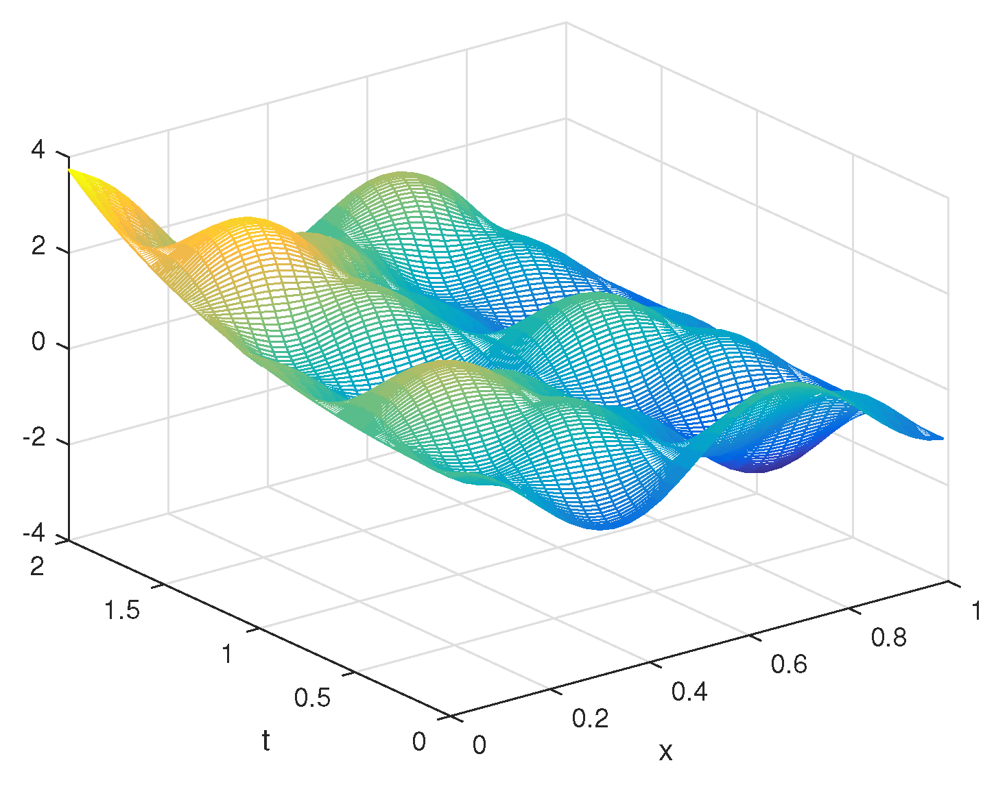
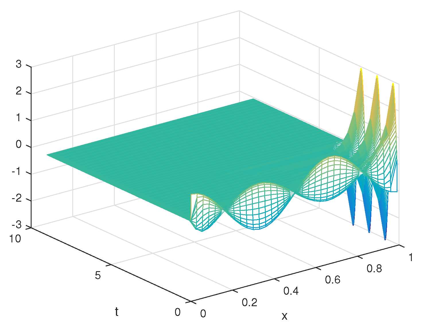
5. Numerical Results

Within this section, mathematical simulations are conducted to verify the efficacy of the proposed control law. The dynamical behavior of system (1) is simulated using the following parameters:

$$q(y,0)=q_0\left(y\right)=cos\left(3\pi y\right),q_t(y,0)=q_1\left(y\right)=sin\left(3\pi y\right),$$

$$ϵ=3,b=3,\theta =3,j\left(s\right)=sin(s-ϵ).$$

In the absence of control function, system (1) is as described below:

$$\left\{\begin{array}{ccc}{q}_{tt}(y,t)=q_{yy}(y,t),\hfill & y\in (0,1),t>0,\hfill & \hfill \\ q(0,t)=0,q(1,t)=0,\hfill & t>0,\hfill \\ q(y,0)=cos\left(3\pi y\right),q_t(y,0)=sin\left(3\pi y\right),\hfill & y\in (0,1),\hfill \\ \psi (s-3)=sin(s-3).\hfill & s\in (0,3).\hfill \end{array}\right.$$

(21)

The resulting figure is shown in Figure 1.

For the control function, system (1) is as described below:

$$\left\{\begin{array}{cc}{q}_{tt}(y,t)=q_{yy}(y,t),\hfill & y\in (0,1),t>0,\hfill \\ q(0,t)=0,q(1,t)=\psi \left(t\right)+\psi (t-3),\hfill & \hfill \\ q(y,0)=cos\left(3\pi y\right),q_t(y,0)=sin\left(3\pi y\right),\hfill & y\in (0,1),\hfill \\ \psi (s-3)=sin(s-3),\hfill & s\in (0,3).\hfill \end{array}\right.$$

(22)

The resulting figure is shown in Figure 2.

All computations are implemented in MATLAB R2016a. The implicit Euler method and central finite difference approximations are employed, with the temporal and spatial grid sizes set to $dy=0.03$ and $dt=0.01,$ respectively. In Figure 1, no controller is applied, indicating that the system is unstable. The addition of a controller in Figure 2 shows that the system becomes stable. Therefore, the results in the figure above illustrate the effectiveness of the controller developed in this study.

6. Conclusions

The stability problem of a wave equation featuring boundary difference-type delay control is investigated in this study. We conclude that under the action of the integral feedback controller (3), the original system (1) achieves exponential stability, which has been verified by numerical simulations. Therefore, the controller designed in this article is effective.

Unlike traditional dynamic controller design, our approach establishes an equivalence between the system under study and a target system. The key advantage of our controller design method lies in its ability to ensure the stability of the original system by guaranteeing the stability of the target system. The primary challenge lies in rigorously proving the equivalence between the two systems. In future work, we aim to explore the design of more sophisticated control structures.

References

1. Russell, D.L. Mathematical models for the elastic beam and their control-theoretic implications. Semigroups. Theory Appl. 1986, 2, 177–216. [Google Scholar]
2. Lions, J.L. Exact controllability, stabilization and perturbations for distributed systems. SIAM Rev. 1988, 30, 1–68. [Google Scholar]
3. Malek-Zavarei, M.; Jamshidi, M. Time-Delay Systems: Analysis, Optimization and Applications; Elsevier Science Inc.: Amsterdam, The Netherlands, 1987. [Google Scholar]
4. Michiels, W.; Niculescu, S.I. Stability and Stabilization of Time-Delay Systems: An Eigenvalue-Based Approach; SIAM: Bangkok, Thailand, 2007. [Google Scholar]
5. Datko, R.; Lagnese, J.; Polis, M. An example on the effect of time delays in boundary feedback stabilization of wave equations. SIAM J. Control Optim. 1986, 24, 152–156. [Google Scholar]
6. Datko, R. Two examples of ill-posedness with respect to small time delays in stabilized elastic systems. IEEE Trans. Autom. Control 1993, 38, 163–166. [Google Scholar]
7. Logemann, H.; Rebarber, R.; Weiss, G. Conditions for robustness and nonrobustness of the stability of feedback systems with respect to small delays in the feedback loop. SIAM J. Control Optim. 1996, 34, 572–600. [Google Scholar]
8. Brahmi, B.; Driscoll, M.; Laraki, M.H.; Brahmi, A. Adaptive high-order sliding mode control based on quasi-time delay estimation for uncertain robot manipulator. Control Theory Technol. 2020, 18, 279–292. [Google Scholar]
9. Sheng, Z.; Guo, Y.; Xue, A.; Han, W. Multi-sensor multi-target bearing-only tracking with signal time delay. Signal, Image Video Process. 2023, 17, 4495–4502. [Google Scholar] [CrossRef]
10. Xia, Y.; Zhang, X.; Xia, S.; Wu, M.; Feng, Y. Pathological basal ganglia oscillations with time delays: A memoryless feedback control strategy. Control Theory Technol. 2024, 22, 1–13. [Google Scholar]
11. Komornik, V. On the Nonlinear Boundary Stabilization of the Wave-Equation. Chin. Ann. Math. Ser. 1993, 14, 153–164. [Google Scholar]
12. Komornik, V. Rapid boundary stabilization of linear distributed systems. SIAM J. Control Optim. 1997, 35, 1591–1613. [Google Scholar]
13. Lasiecka, I.; Triggiani, R. Control Theory for Partial Differential Equations: Continuous and Approximation Theories. Encyclopedia of Mathematics and its Applications; Cambridge University Press: Cambridge, UK, 2000. [Google Scholar]
14. Kobayashi, T. Stabilization of infinite-dimensional undamped second order systems by using a parallel compensator. Ima J. Math. Control Inf. 2004, 1, 85–94. [Google Scholar]
15. Xu, G.Q. Stabilization of string system with linear boundary feedback. Nonlinear Anal. Hybrid Syst. 2007, 1, 383–397. [Google Scholar]
16. Rebarber, R.; Townley, S. Robustness with respect to delays for exponential stability of distributed parameter systems. SIAM J. Control Optim. 1998, 37, 230–244. [Google Scholar]
17. Dastan, Z.; Tavakoli-Kakhki, M. Suppression of high order disturbances and tracking for nonchaotic systems: A time-delayed state feedback approach. Control Theory Technol. 2022, 20, 54–68. [Google Scholar]
18. Guo, B.Z.; Xu, C.Z.; Hammouri, H. Output feedback stabilization of a one-dimensional wave equation with an arbitrary time delay in boundary observation. ESAIM Control Optim. Calc. Var. 2022, 18, 22–35. [Google Scholar]
19. Lhachemi, H.; Prieur, C. Boundary output feedback stabilisation of a class of reaction–diffusion PDEs with delayed boundary measurement. Int. J. Control 2023, 96, 2285–2295. [Google Scholar]
20. Xu, G.Q.; Yung, S.P.; Li, L.K. Stabilization of wave systems with input delay in the boundary control. ESAIM Control Optim. Calc. Var. 2006, 12, 770–785. [Google Scholar]
21. Nicaise, S.; Pignotti, C. Stability and instability results of the wave equation with a delay term in the boundary or internal feedbacks. SIAM J. Control Optim. 2006, 45, 1561–1585. [Google Scholar]
22. Shang, Y.F.; Xu, G.Q. Stabilization of an Euler–Bernoulli beam with input delay in the boundary control. Syst. Control Lett. 2012, 61, 1069–1078. [Google Scholar]
23. Wang, H.; Xu, G.Q. Exponential stabilization of 1-d wave equation with input delay. WSEAS Trans. Math. 2013, 12, 1001–1013. [Google Scholar]
24. Liu, X.F.; Xu, G.Q. Exponential stabilization for Timoshenko beam with distributed delay in the boundary control. Abstr. Appl. Anal. 2013, 2013, 726794. [Google Scholar] [CrossRef]
25. Han, Z.J.; Xu, G.Q. Output-based stabilization of Euler–Bernoulli beam with time-delay in boundary input. IMA J. Math. Control Inf. 2014, 31, 533–550. [Google Scholar] [CrossRef]
26. Shang, Y.F.; Xu, G.Q. Dynamic feedback control and exponential stabilization of a compound system. J. Math. Anal. Appl. 2015, 422, 858–879. [Google Scholar] [CrossRef]
27. Guo, Y.; Xu, G.; Guo, Y. Stabilization of the wave equation with interior input delay and mixed Neumann-Dirichlet boundary. Discret. Contin. Dyn. Syst.-B 2016, 21, 2491–2507. [Google Scholar] [CrossRef]
28. Liu, X.P.; Xu, G.Q. Integral-Type Feedback Controller and Application to the Stabilization of Heat Equation with Boundary Input Delay. WSEAS Trans 2018, 17, 311–318. [Google Scholar]
29. Feng, X.; Xu, G.; Chen, Y. Rapid stabilisation of an Euler–Bernoulli beam with the internal delay control. Int. J. Control 2019, 92, 42–55. [Google Scholar]
30. Chen, H.; Xie, Y.; Genqi, X. Rapid stabilisation of multi-dimensional Schrödinger equation with the internal delay control. Int. J. Control 2019, 92, 2521–2531. [Google Scholar]
31. Liu, X.P.; Xu, G.Q. Solvability of the nonlocal initial value problem and application to design of controller for heat-equation with delay. J. Math. Study 2019, 52, 127–159. [Google Scholar]
32. Zhang, L.; Xu, G.Q.; Chen, H. Uniform stabilization of 1-d wave equation with anti-damping and delayed control. J. Frankl. Inst. 2020, 357, 12473–12494. [Google Scholar] [CrossRef]
33. Xu, G.Q.; Zhang, L. Uniform stabilization of 1-D coupled wave equations with anti-dampings and joint delayed control. SIAM J. Control Optim. 2020, 58, 3161–3184. [Google Scholar] [CrossRef]
34. Zhang, L.; Xu, G.Q.; Mastorakis, N.E. A new approach for stabilization of Heat-ODE cascaded systems with boundary delayed control. IMA J. Math. Control Inf. 2022, 39, 112–131. [Google Scholar]
35. Xie, Y.; Chen, Y. Rapid Stabilization of Timoshenko Beam System with the Internal Delay Control. Acta Appl. Math. 2023, 186, 7. [Google Scholar] [CrossRef]
36. Pazy, A. Semigroups of Linear Operators and Applications to Partial Differential Equations; Springer-Verlag: Berlin/Heidelberg, Germany, 1983. [Google Scholar]
37. Smyshlyaev, A.; Cerpa, E.; Krstic, M. Boundary Stabilization of a 1-D Wave Equation with In-Domain Antidamping. SIAM J. Control Optim. 2010, 48, 4014–4031. [Google Scholar] [CrossRef]
Figure 1. q ( y , t ) without control law.
Axioms 14 00280 g001
Figure 2. q ( y , t ) with control.
Axioms 14 00280 g002
Disclaimer/Publisher’s Note: The statements, opinions and data contained in all publications are solely those of the individual author(s) and contributor(s) and not of MDPI and/or the editor(s). MDPI and/or the editor(s) disclaim responsibility for any injury to people or property resulting from any ideas, methods, instructions or products referred to in the content.