Abstract
This article investigates and analyzes the diverse patterns of Julia sets generated by new classes of generalized exponential and sine rational functions. Using a generalized viscosity approximation-type iterative method, we derive escape criteria to visualize the Julia sets of these functions. This approach enhances existing algorithms, enabling the visualization of intricate fractal patterns as Julia sets. We graphically illustrate the variations in size and shape of the images as the iteration parameters change. The new fractals obtained are visually appealing and attractive. Moreover, we observe fascinating behavior in Julia sets when certain input parameters are fixed, while the values of n and m vary. We believe the conclusions of this study will inspire and motivate researchers and enthusiasts with a strong interest in fractal geometry.
Keywords:
algorithms; escape criteria; Julia sets; iterative methods; generalized rational functions MSC:
28A80; 37F10; 39B12; 47H10
1. Introduction
Fractal geometry challenges the traditional notion that nature adheres to simple geometric forms, instead unveiling its true complexity through intricate, irregular patterns. By embracing self-similarity across scales, fractal geometry provides a powerful framework for analyzing shapes that defy classical classification. It reveals structured, yet seemingly chaotic, patterns inherent in the natural world, offering a unique perspective on its richness and complexity. This holistic approach deepens our understanding of the principles underlying various natural phenomena. Fractal analysis spans numerous disciplines, from science to art, expanding our perception of the world and highlighting the interconnectedness of diverse patterns. For further insights, see [1,2,3]. The allure of fractals, particularly Julia and Mandelbrot sets, has captivated mathematicians for decades. The foundation of Julia sets traces back to the early 20th-century work of the French mathematician Gaston Julia [4].
The construction of fractals, including Mandelbrot and Julia sets, is founded on various fixed-point iterative methods. Techniques such as Mann iteration, Picard iteration, and others (see [5,6,7,8,9,10]) have been extensively applied by mathematicians to analyze the behavior and patterns of polynomials, complex sine and cosine functions, and transcendental functions. These approaches reveal that the shape, color, and other characteristics of fractals can vary significantly depending on the iterative method applied to the same function (see [11,12]). In addition to Julia sets, iteration schemes play a key role in generating other fractals, including biomorphs, iterated function system fractals, inversion fractals, and root-finding fractals (see [13,14]).
In 2000, Moudafi [15] explored the convergence properties of the viscosity method in the framework of semi-nonexpansive mappings, providing valuable insights into iterative techniques. These advancements have greatly enriched the study and applications of fractals, enhancing our understanding of their intricate structures. More recently, Nandal et al. [16] proposed a generalized version of viscosity approximation-type iterative methods in the context of Hilbert spaces, significantly expanding both the theoretical foundation and practical applications of this approach.
The study revealed the untapped potential of the method for fractal generation. This intriguing connection suggests that the generalized viscosity approximation-type iterative method can not only solve complex problems in optimization and nonlinear analysis but also serve as a powerful tool for exploring and constructing fractals, such as Julia sets and related structures. Furthermore, the generalized viscosity approximation-type iterative method is a significant extension of classical fixed-point methods, including Halpern’s iteration and other iterative techniques.
The method allows for the more efficient and flexible exploration of fractal structures, revealing intricate, self-similar patterns that are difficult to achieve with more traditional methods, and the convergence properties of the generalized viscosity approximation method help in generating fractals with greater precision, making it possible to visualize even subtle variations in the fractal patterns as Julia sets. Julia sets are remarkable mathematical formations generated through iterative processes, showcasing intricate and mesmerizing fractal patterns. These sets arise by repeatedly applying a function to complex numbers, with each iteration determining whether a particular number stays bounded or escapes to infinity.
In recent studies, Kumari et al. [17,18] and Iqbal et al. [19] investigated the application of generalized viscosity approximation-type iterative methods in fractal generation, emphasizing their potential in producing Mandelbrot and Julia sets. In their subsequent research, these methods were applied to analyze and visualize the intricate dynamics of Julia and Mandelbrot sets, contributing to a deeper understanding of these captivating fractal structures. Building on this work, the present study adapts the existing viscosity approximation-type iterative method to establish escape criteria for the new generalized exponential rational function and the generalized sine rational function where These functions are analytic except at
The structure of the paper is organized as follows: Section 2 introduces the fundamental definitions and preliminary results necessary to achieve the goals of this study. Section 3 establishes the main theorems used to derive a general escape criterion, which is crucial for generating Julia sets through a viscosity approximation-type iterative method. Section 4 details the algorithms implemented and presents visual illustrations of Julia sets generated using MATLAB R2019a (9.6.0.1072779, 64-bit) for various parameter values, along with a comprehensive discussion of the results. Finally, Section 5 concludes the paper with a summary of the key findings.
2. Preliminaries
This section presents some fundamental definitions and essential results that are necessary to accomplish the objectives of this article.
Definition 1
(Julia set [4]). Let be a complex-valued function. The filled Julia set of W is defined as
where denotes the compositional iterate of W. The Julia set is the boundary of the filled Julia set.
Definition 2.
Let be a complex-valued function and an initial point. Define the following sequence:
The escape time for is the minimum integer p such that , where R is a predefined escape radius. If the point is said to escape to infinity under iteration. If the point does not escape within a maximum number of iterations K, it is assumed to belong to the filled Julia set.
Definition 3
([15]). Let denote the sequence of iterates, with as the initial point. The sequence is said to follow the viscosity approximation method if
where g, and W are self-mappings on , with g being a contraction mapping.
This iterative process, introduced by Moudafi [15] in combines the contraction mapping g with the operator W through a convex combination that evolves with each iteration.
A novel generalized viscosity approximation-type iterative method was studied by Nandal et al. [16]. This approach can be described in the complex plane as follows: starting from an initial point the sequence is defined by
where and for with the resolvent operators and are associated with monotone operators and respectively, with
Consider the following new class of complex functions which are analytic except at as
and
where and
The key to generating fractals and establishing escape criteria lies in running the algorithms effectively. It is well known that for certain values of . The Maclaurin series expansions for the exponential and sine functions are given by
where except the values of for which and
where except the values of for which (see the details [5]).
3. Main Results
In this section, we construct an escape time algorithm based on the iteration scheme (3) to analyze the newly introduced generalized exponential and sine rational functions.
Assume and let the sequences be constant, given by where , and Suppose that the function is a contraction mapping with and and define and where Accordingly, we have and Furthermore, let and where Q and W are defined in (4) and (5), respectively. Under these assumptions, the iterative scheme given by (3) takes the following form:
where and
3.1. Escape Criteria for
In this subsection, we derive the escape criterion for the function using (8).
Theorem 1.
Let , where , and let be a complex contraction mapping with and Then, the sequence defined by the iteration in (8), satisfies as
Proof.
From the definition of we have
For and using (6), we obtain
Our assumption yields that and and we obtain
and thus,
Thus, we have
Our assumption gives
From (10), we obtain
Now, based on the construction of we have
The assumption yields that and and therefore, we obtain
Now, based on the construction of we have
Therefore,
Further, from (8), consider
From (15), we have
From (14), we have
Our assumptions give
Thus, there exists such that
In particular, Continuing this procedure, we obtain Hence, as □
In the proof of Theorem 1, we rely solely on the fact that Therefore, this result can be refined to yield the following corollary.
Corollary 1.
Let Then, as
3.2. Escape Criteria for
In this subsection, we derive the escape criterion for using (8).
Theorem 2.
Let , , where and let be a complex contraction mapping with and Then, as where is defined in (8).
Proof.
Based on the construction of we have
For and using (7), we obtain
Our assumption yields that and and and we obtain
and thus,
Thus, we have
Our assumption gives
From (19), we obtain
Now, based on the construction of we have
The assumption yields that and and therefore, we obtain
Now, based on the construction of we have
Therefore,
Further, from (8), consider
From (24), we have
From (23), we have
Our assumptions give
Thus, there exist such that
In particular, Continuing this procedure, we obtain Hence, as □
In the proof of Theorem 2, we relied solely on the fact that So, we can refine it and obtain the following corollary.
Corollary 2.
Let Then, as
4. Graphical Examples
To visualize fractals, specific convergence conditions are crucial, serving as the foundation for effectively executing the algorithm and generating the desired fractal structures. We construct and analyze Julia sets corresponding to various parameter values, examining how these variations influence the resulting patterns. The Julia sets are computed using the generalized viscosity approximation-type iterative method given in (8), with a maximum of 70 iterations applied throughout this work. All fractal visualizations are produced using MATLAB R2019a (9.6.0.1072779, 64-bit), which enables the generation of non-classical Julia sets across distinct orbits. To carry out these visualizations, we develop two dedicated algorithms: one for the Julia set of , and another for , where and By varying the input parameters along with the values of n and m, we present the resulting Julia sets produced by Algorithms 1 and 2.
| Algorithm 1 Julia set generation for |
| Input: where -area in which we draw |
| the set; K-maximal number of iterations; ; , where |
| with colormap -color with C colors. |
| Output: Julia set for area A |
| for do |
| R = |
| k=0 |
| while do |
| , where |
| if then break end if |
| k=k+1 |
| color with colormap |
| Algorithm 2 Julia set generation for . |
| Input: where -area in which we |
| draw the set; K-maximal number of iterations; ; , where |
| with colormap -color with C colors. |
| Output: Julia set for area A |
| for do |
| R = |
| k=0 |
| while do |
| , where |
| if then break end if |
| k=k+1 |
| color with colormap |
4.1. Julia Sets for
This subsection presents the Julia sets corresponding to the generalized exponential rational function for different input values. The execution times for generating these images are also provided in seconds.
In the first example, we generate Julia sets using Algorithm 1 for the functions and . The parameter values used for this illustration are The resulting images are organized into four groups. In each group, three of the parameters from are held fixed, while the fourth is varied:
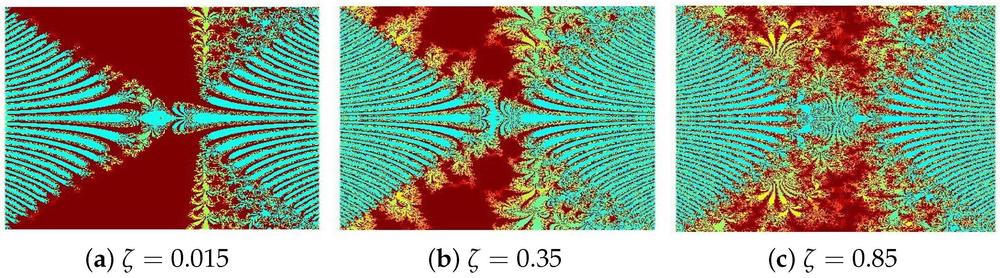
- In Figure 1, are fixed, and is varying: (a) (b) and (c)
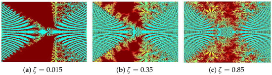 Figure 1. Julia sets generated via Algorithm 1 with fixed values of , , , and varying . Image execution times are as follows: (a) 2.14 s, (b) 2.41 s, and (c) 2.83 s.
 - In Figure 2, are fixed, and is varying: (a) (b) and (c)
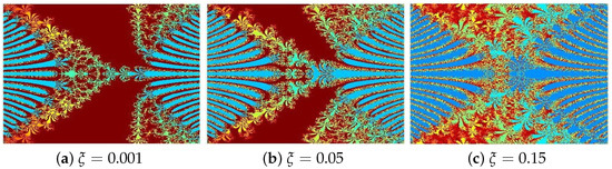 Figure 2. Julia sets generated via Algorithm 1 with fixed values of and varying . The image execution times are as follows: (a) 1.92 s, (b) 2.12 s, and (c) 2.33 s.
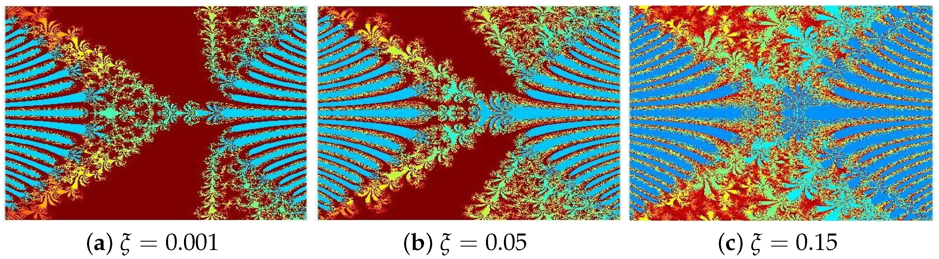
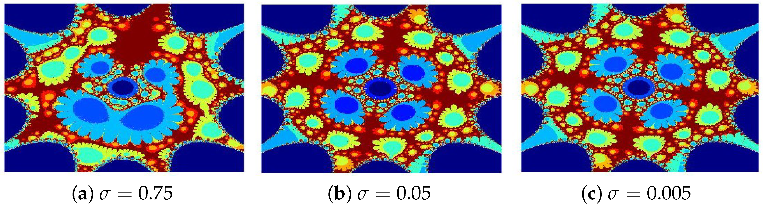
 - In Figure 3, are fixed and is varying: (a) (b) and (c)
 Figure 3. Julia sets generated via Algorithm 1 with fixed values of and varying Image execution times are as follows: (a) 2.04 s, (b) 2.26 s, and (c) 2.43 s.
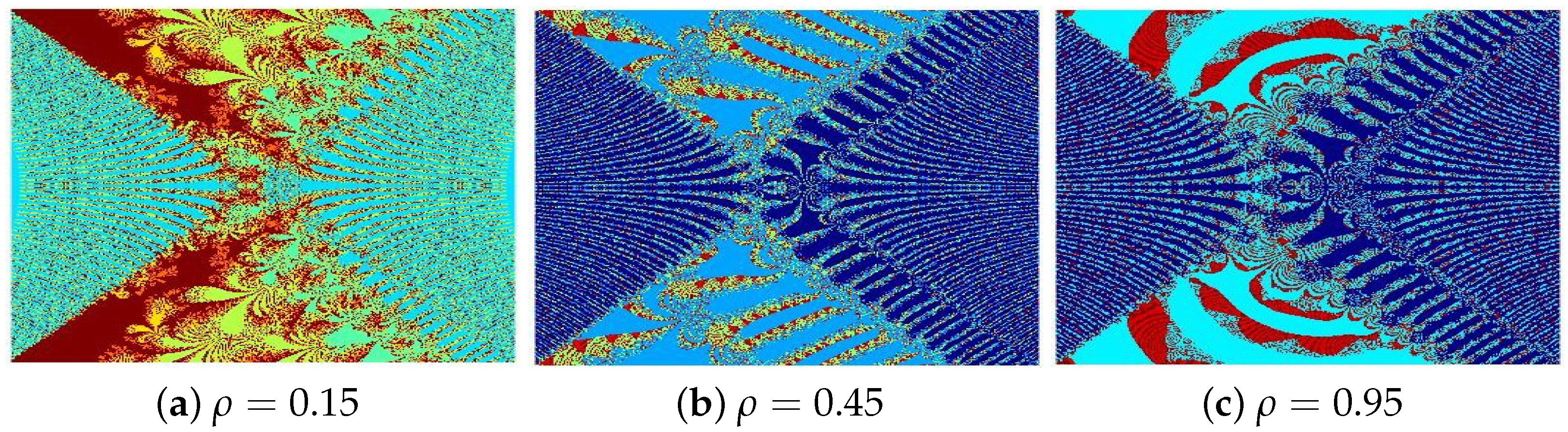
 - In Figure 4, are fixed and is varying: (a) (b) (c)
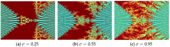 Figure 4. Julia sets generated via Algorithm 1 with fixed values of and varying Image execution times are as follows: (a) 2.21 s, (b) 2.61 s, and (c) 2.95 s.
In Figure 1, Figure 2, Figure 3 and Figure 4a–c, for and we fix the values of three parameters from and vary the remaining one. It is clear that the four parameters and play a significant role in determining the shape, size, and color of the sets. As shown in these figures, an increase in any of the parameters leads to an expansion of the set, accompanied by changes in its shape. The image generation time for each iteration is also recorded.
In the second example, we generate Julia sets using Algorithm 1 for the functions and . The parameter values used for this illustration are The resulting images are organized into three groups. In each group, two of the parameters from are held fixed, while the fourth is varied:
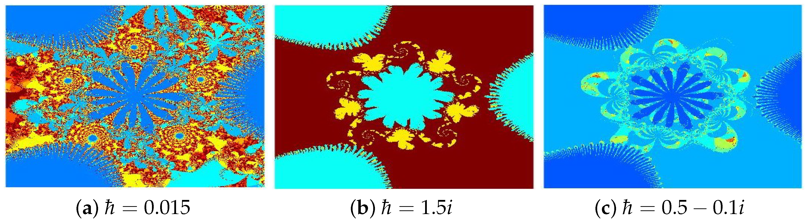
- In Figure 5, with fixed, ℏ is varied as follows: (a) (b) (c)
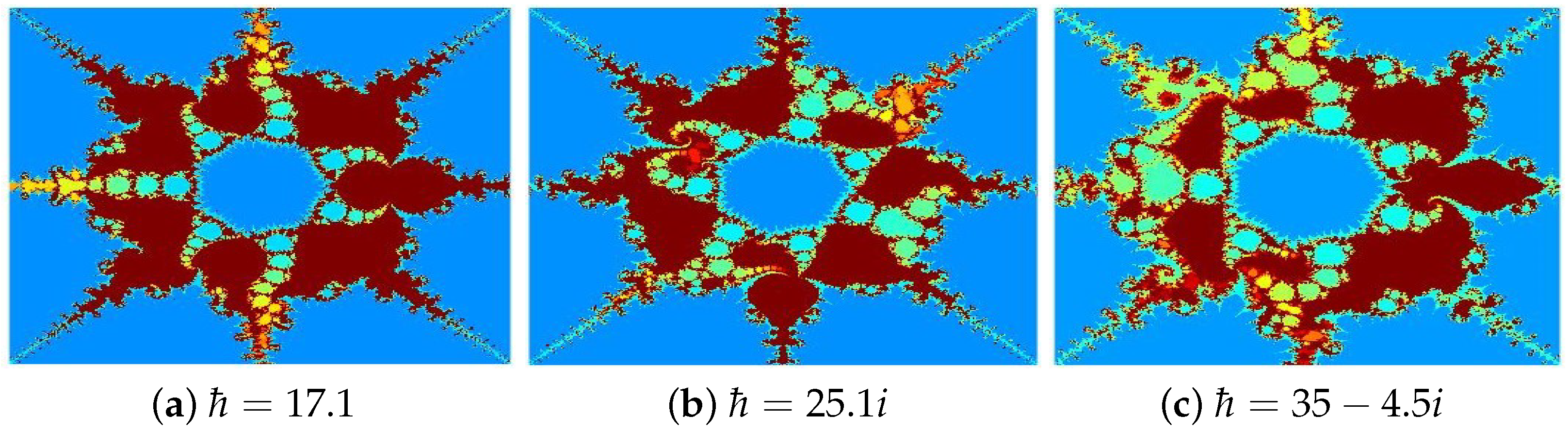
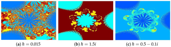 Figure 5. Julia sets generated via Algorithm 1 with fixed values of , , and varying ℏ. Image execution times are as follows: (a) 3.01 s, (b) 3.18 s, and (c) 3.32 s.
 - In Figure 6, with fixed, ℘ is varied as follows: (a) (b) (c)
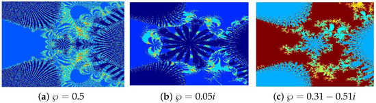 Figure 6. Julia sets generated via Algorithm 1 with fixed values of , , and varying ℘. Image execution times are as follows: (a) 3.21 s, (b) 3.54 s, and (c) 3.87 s.
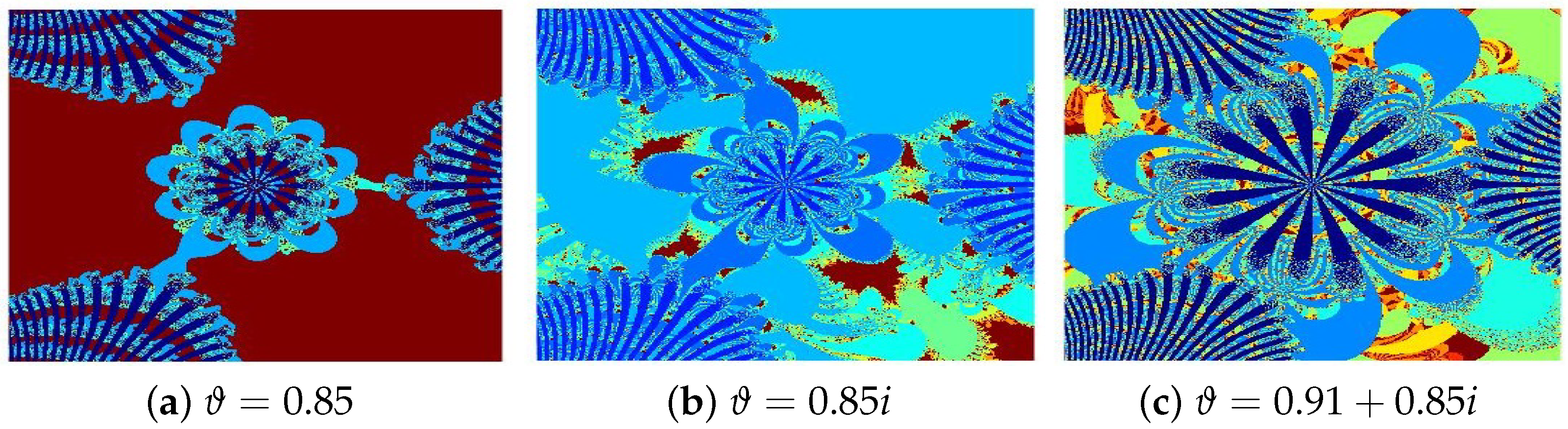
 - In Figure 7, with fixed, is varied as follows: (a) (b) and (c)
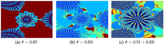 Figure 7. Julia sets generated via Algorithm 1 with fixed values of , , and varying . Image execution times are as follows: (a) 3.21 s, (b) 3.54 s, and (c) 3.87 s.
In Figure 5, Figure 6 and Figure 7a–c, with and , we present Julia sets generated by fixing two of the parameters or , while varying the third. Specifically, in subfigures (a), the parameters are set as purely real, in (b) as purely imaginary, and in (c) as complex values. These variations highlight the significant influence of , and on the geometry, scale, and coloration of the Julia sets particularly around the edges of the characteristic leaf-like structures. The resulting patterns resemble traditional Rangoli designs, floral motifs, or intricate stained glass artwork. The execution times for each image are recorded per iteration to support the detailed performance analysis.
In the third example, we generate Julia sets using Algorithm 1 for the function . The parameter values used for this illustration are The resulting images are organized into two groups. In each group, one of the parameters from r and s is held fixed, while the second is varied:
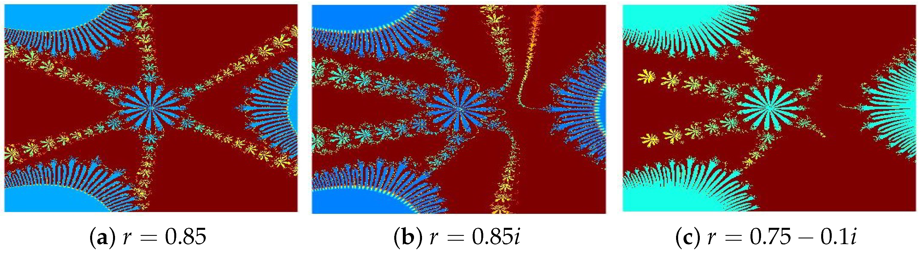
- In Figure 8, is fixed, and r is varied: (a) (b) and (c)
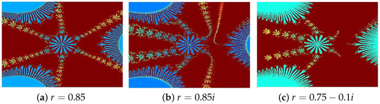 Figure 8. Julia sets generated via Algorithm 1 with fixed values of , and varying r. Image execution times are as follows: (a) 1.18 s, (b) 1.23 s, and (c) 1.29 s.
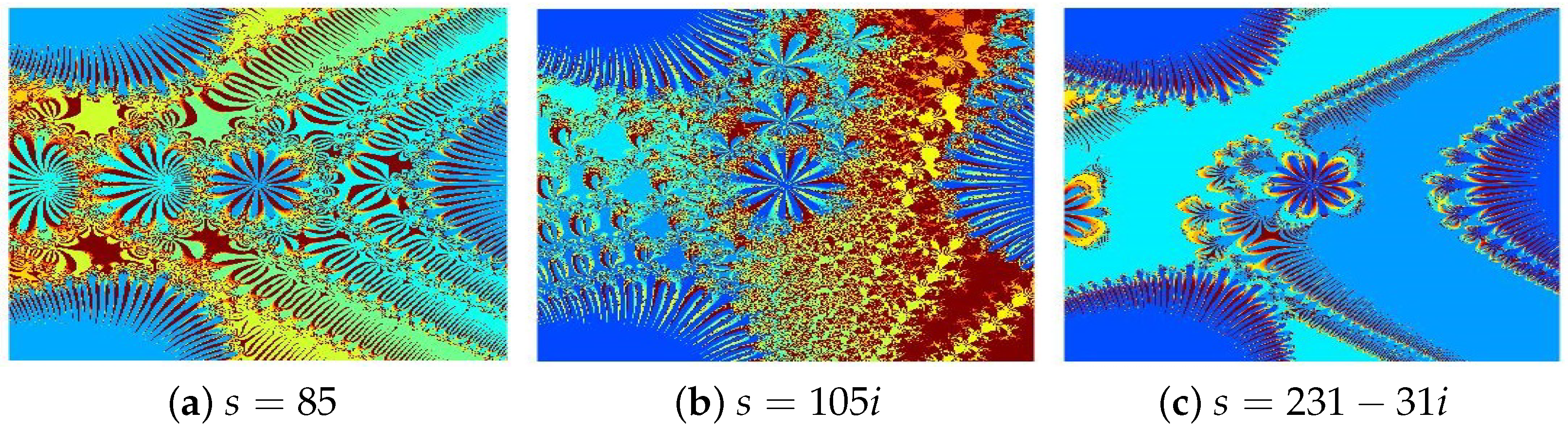
 - In Figure 9, is fixed, and s is varied: (a) (b) and (c)
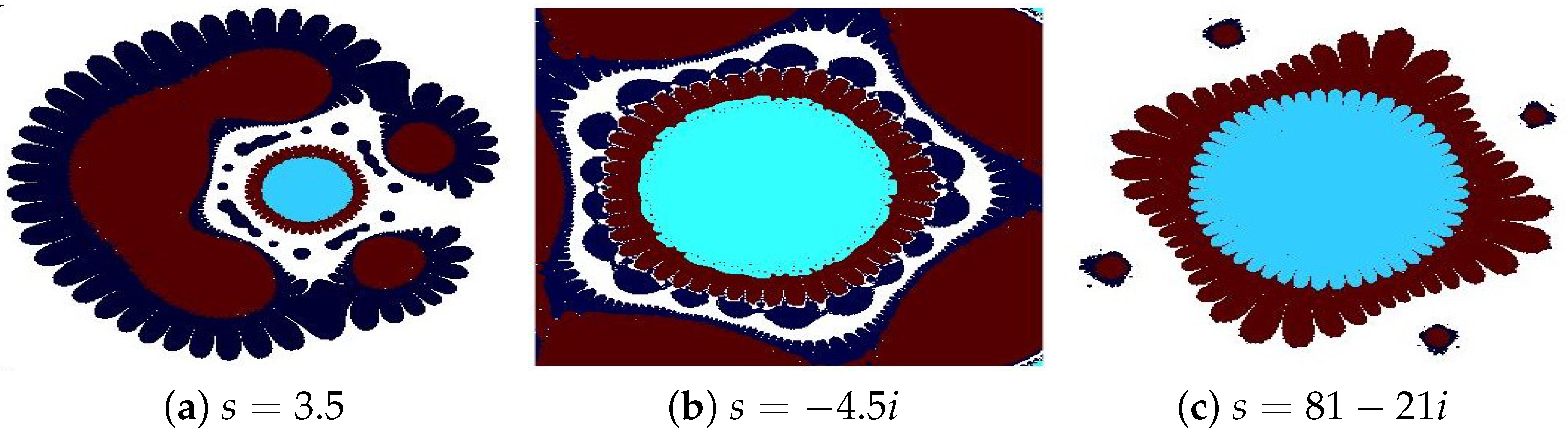
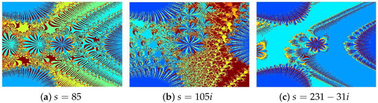 Figure 9. Julia sets generated via Algorithm 1 with fixed values of , and varying s. Image execution times are as follows: (a) 1.34 s, (b) 1.68 s, and (c) 1.76 s.
In Figure 8a–c and Figure 9a–c, with and , we display Julia sets produced by fixing one of the parameters r or s, while varying the other. In subfigures (a), both r and s are set as purely real, in (b) as purely imaginary, and in (c) as complex values. These variations clearly demonstrate that the parameters r and s significantly affect the structure, scale, and color distribution of the Julia sets, particularly along the contours of the leaf-like formations. The generated patterns resemble traditional Rangoli designs, floral arrangements, or delicate stained glass artwork.
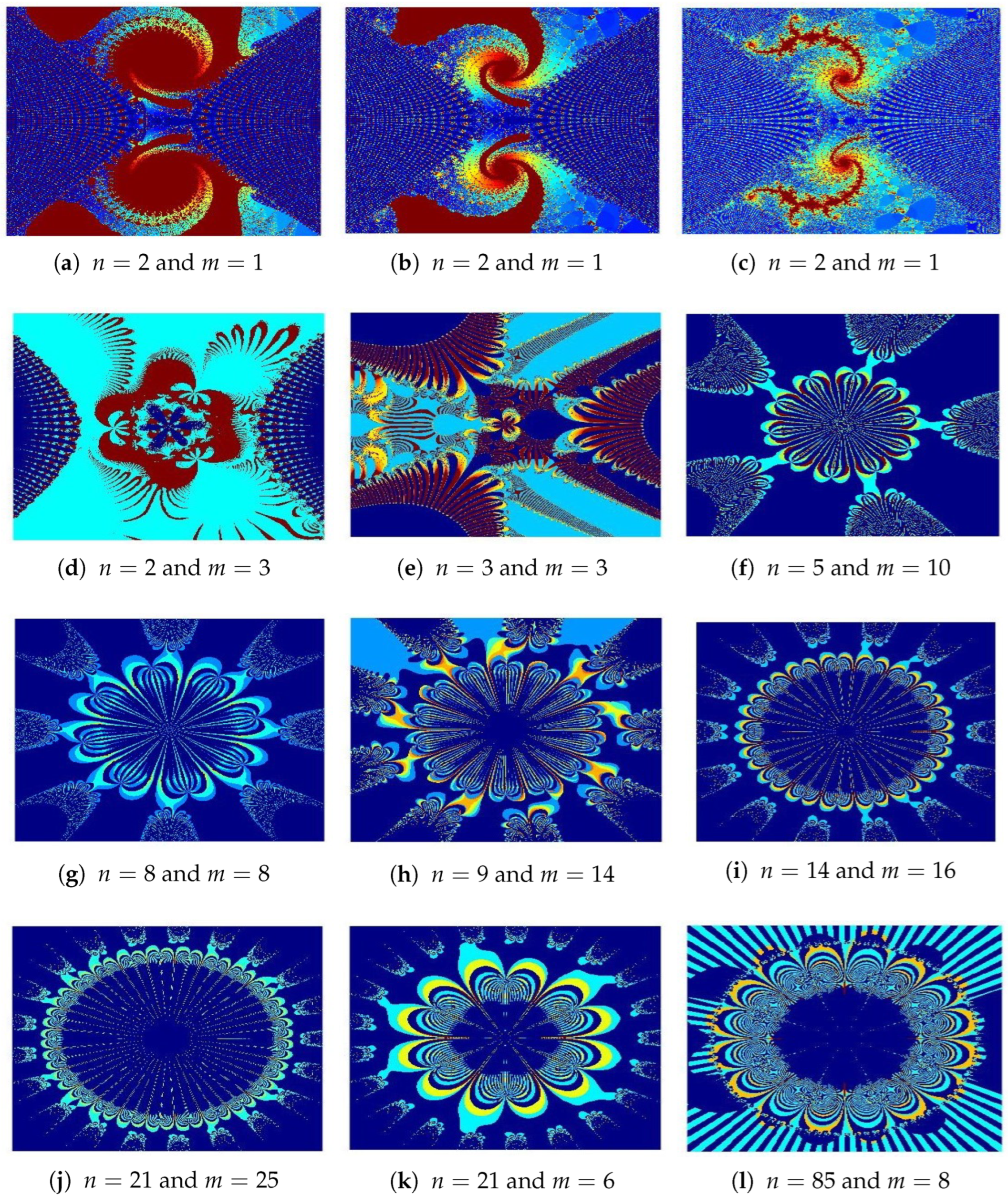
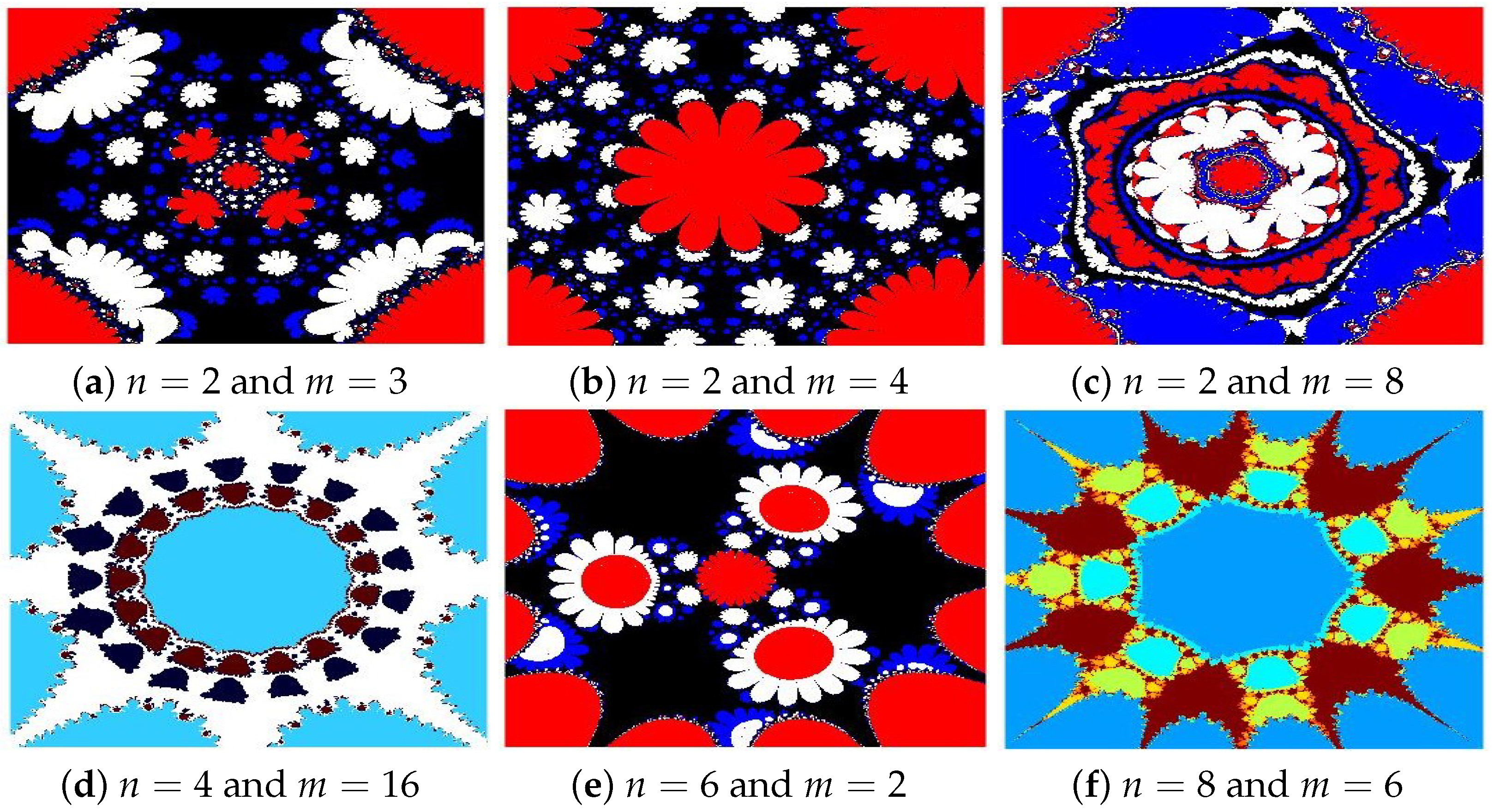
In this example, we showcase the diversity of Julia sets generated using the generalized viscosity approximation-type iterative method for and These sets are illustrated in Figure 10a–l, with the parameters used for their generation specified as follows:

Figure 10.
Julia sets generated via Algorithm 1 with varying n and m. Image execution times are as follows: (a) 2.23 s, (b) 2.58 s, (c) 2.76 s, (d) 3.02 s, (e) 3.48 s, (f) 3.87 s, (g) 4.23 s, (h) 4.58 s, (i) 5.07 s, (j) 5.17 s, (k) 5.26 s, and (l) 5.47 s.
- (a)
- (b)
- (c)
- (d)
- (e)
- (f)
- (g)
- (h)
- (i)
- (j)
- (k)
- (l)
In Figure 10a–e, we observe distinct behavioral changes in the Julia sets when varying the parameters in the generalized exponential rational function via Algorithm 1. Adjusting the values of parameter and b as purely real, purely imaginary, and complex lead to noticeable differences in the color, shape, and size of the Julia sets. The resulting images display intricate and beautiful fractal patterns. Figure 10f–l illustrate Julia sets for even/odd, while the other parameters remain fixed as described in Figure 10f–l. From these images, it is clear that as n and m increase, and the sets evolve into circular shapes, with petal counts corresponding to the values of n and m. Furthermore, the number of petals increases as n and m increase. The generated Julia sets are strikingly complex, resembling traditional Rangoli patterns, floral shapes, or intricate glass art. Additionally, the image generation time is recorded, showing an increase with each iteration.
4.2. Julia Sets for
The Julia sets corresponding to the generalized sine rational function for different input values are illustrated in this subsection.
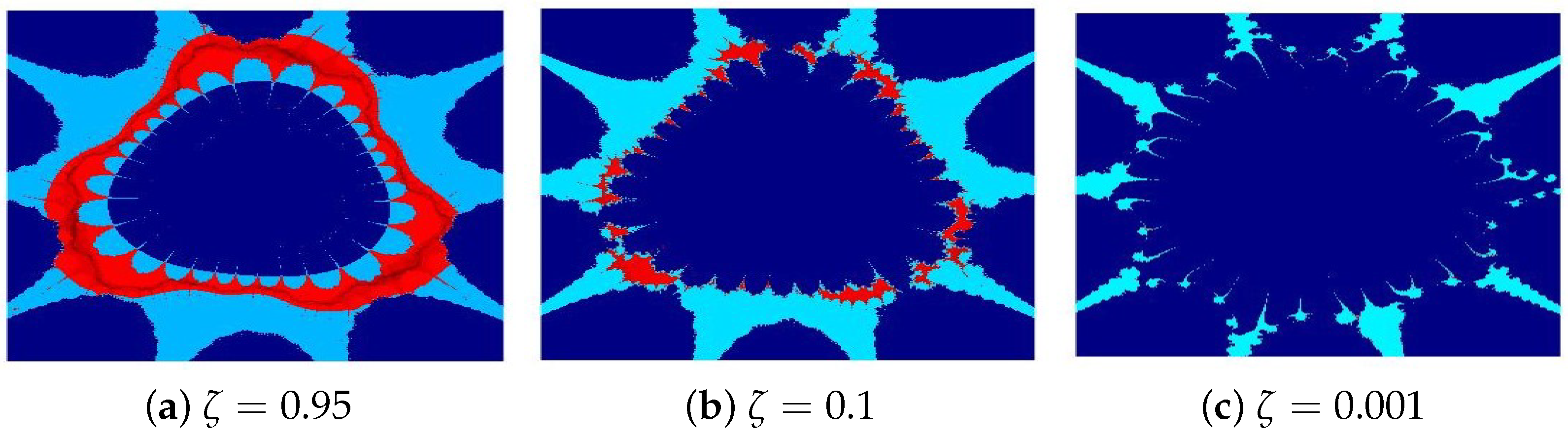
In the first example, we generate Julia sets via Algorithm 2 for the function and a complex contraction mapping . The parameter values used for this illustration are The generated images are categorized into four groups. In each group, three parameters of are held fixed, while the fourth is varied:
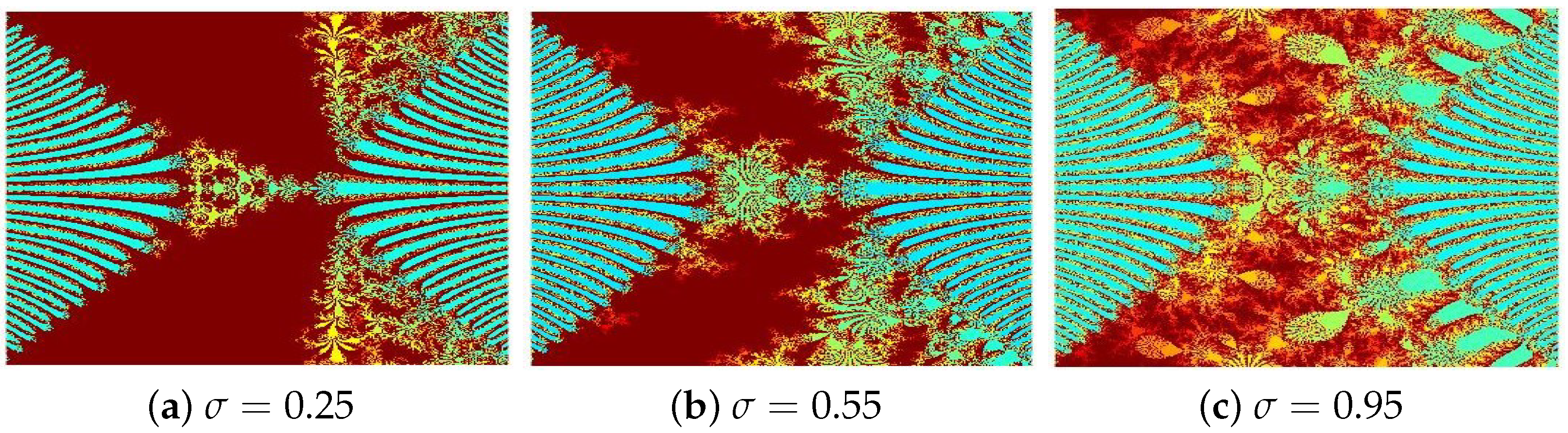
- In Figure 11, are fixed, and is varied as (a) (b) (c)
 Figure 11. Julia sets generated via Algorithm 2 with fixed values of , and varying . Image execution times are as follows: (a) 0.8 s, (b) 0.97 s, and (c) 1.18 s.
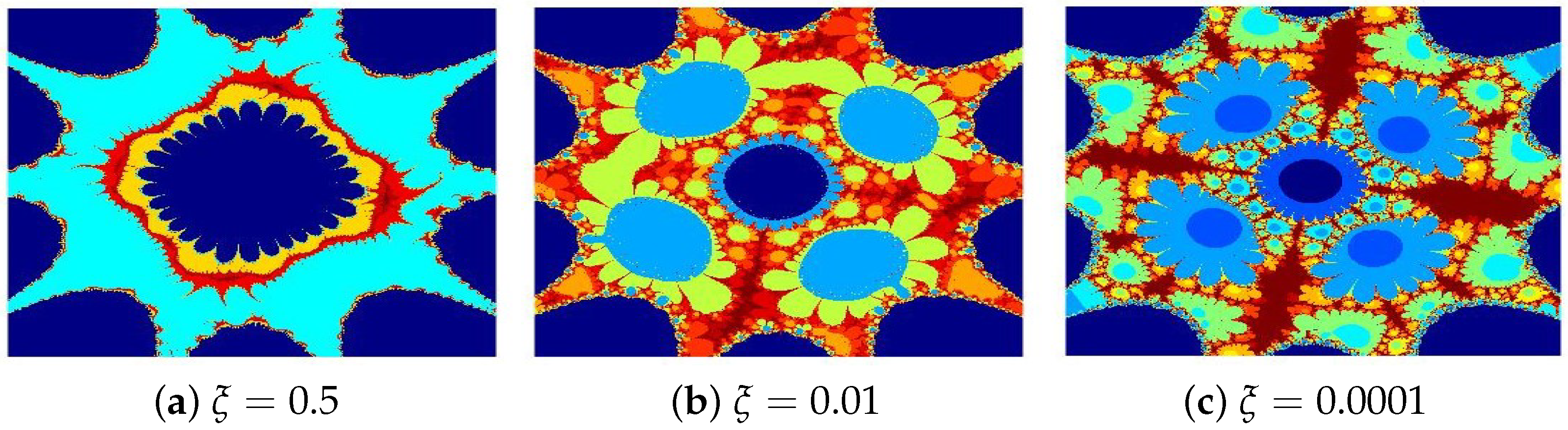
 - In Figure 12, are fixed, and is varied as (a) (b) and (c)
 Figure 12. Julia sets generated via Algorithm 2 with fixed values of and varying . Image execution times are as follows: (a) 1.12 s, (b) 1.32 s, and (c) 1.53 s.
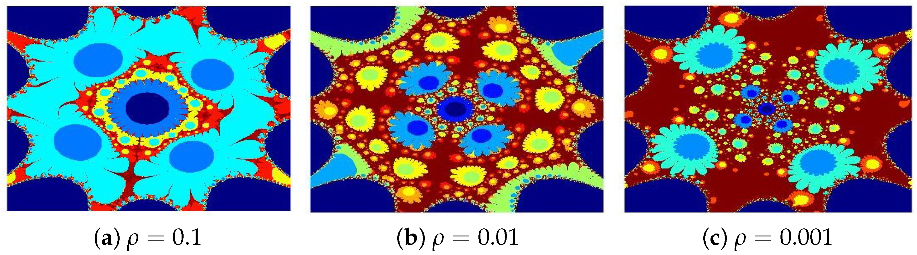
 - In Figure 13, are fixed, and is varied as (a) (b) and (c)
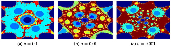 Figure 13. Julia sets generated via Algorithm 2 with fixed values of and varying Image execution times are as follows: (a) 1.52 s, (b) 1.76 s, and (c) 2.13 s.
 - In Figure 14, are fixed, and is varied as (a) (b) and (c)
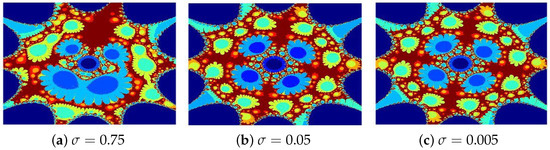 Figure 14. Julia sets generated via Algorithm 2 with fixed values of and varying Image execution times are as follows: (a) 2.01 s, (b) 2.14 s, and (c) 2.25 s.
From Figure 11, Figure 12, Figure 13 and Figure 14a–c, for the fixed values and we observe the impact of varying one parameter from the set while keeping the other three constant. It is evident that these four parameters play a crucial role in shaping the structure of the Julia sets. Specifically, as the values of increase, notable changes occur in the size and form of the fractal bulbs. As illustrated in Figure 11, Figure 12, Figure 13 and Figure 14, the bulb size enlarges with increasing parameter values, accompanied by distinct transformations in shape and visual appearance.
In the second example, the parameters selected for this illustration are as follows: , and The generated images are categorized into three groups. In each group, two parameters from are fixed, while the third is varied:
- In Figure 15, the parameters are fixed, while ℏ is varied as (a) (b) and (c)
 Figure 15. Julia sets generated via Algorithm 2 with fixed values of and varying Image execution times are as follows: (a) 1.21 s, (b) 1.54 s, and (c) 1.77 s.
 - In Figure 16, the parameters are fixed, while ℘ is varied as (a) (b) and (c)
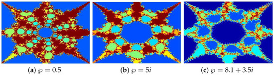 Figure 16. Julia sets generated via Algorithm 2 with fixed values of and varying Image execution times are as follows: (a) 1.61 s, (b) 1.93 s, and (c) 2.27 s.
 - In Figure 17, the parameters are fixed, while is varied as (a) (b) and (c)
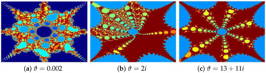 Figure 17. Julia sets generated via Algorithm 2 with fixed values of and varying Image execution times are as follows: (a) 2.41 s, (b) 2.64 s, and (c) 2.87 s.
In the third example, the parameters used to generate the Julia sets in this example are the following: , and The generated images are categorized into four groups. In each group, we fix one of the parameter from while the second is varied:
- In Figure 18, the parameter is fixed, while r is varied as (a) (b) and (c)
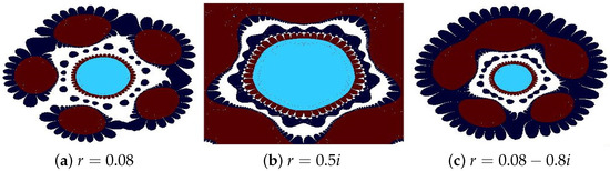 Figure 18. Julia sets generated via Algorithm 2 with fixed values of and varying Image execution times are as follows: (a) 2.61 s, (b) 2.91 s, and (c) 3.11 s.
 - In Figure 19, the parameter is fixed, while s is varied as (a)(b) and (c)
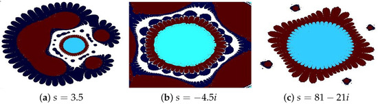 Figure 19. Julia sets generated via Algorithm 2 with fixed values of and varying Image execution times are as follows: (a) 2.89 s, (b) 3.21 s, and (c) 3.31 s.
In Figure 18a–c and Figure 19a–c, Julia sets are displayed for varying parameter configurations: (a) where r, and s are fixed as purely real, (b) as purely imaginary, and (c) as complex values. The central circular region of the Julia sets undergoes noticeable changes, with the surrounding area also transforming in shape and size. These changes often lead to portions detaching from the central structure, forming new, smaller circular regions that bear a resemblance to the original central part.
In this example, we demonstrate the diversity of Julia sets produced using the generalized viscosity approximation-type iterative method for The resulting sets are displayed in Figure 20a–f, generated using the following parameter values:
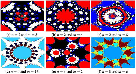
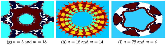
Figure 20.
Julia sets generated via Algorithm 2 with varying n and m. Image execution times are as follows: (a) 2.23 s, (b) 2.58 s, (c) 2.76 s, (d) 3.02 s, (e) 3.48 s, (f) 3.87 s, (g) 4.23 s, (h) 4.58 s, and (i) 5.07 s.
- (a)
- (b)
- (c)
- (d)
- (e)
- (f)
- (g)
- (h)
- (i)
In Figure 15, Figure 16, Figure 17, Figure 18 and Figure 19a–c, we examine Julia sets generated under different parameter conditions: in (a), the parameters ℏ, , and s are fixed as purely real values; in (b), they are set as purely imaginary; and in (c), they take complex values. These variations demonstrate that ℏ, , and s play a crucial role in shaping the structure, scale, and coloration of the Julia sets. Further analysis reveals that adjusting the values of n and m also has a profound effect on the geometry and intricacy of the fractals. As n and m increase, the Julia sets exhibit greater complexity, undergoing significant transformations in their overall form (see Figure 20a–f). The resulting patterns display mesmerizing fractal designs, reminiscent of traditional Rangoli art, floral motifs, or delicate stained glass. The computational time for generating each image is recorded, highlighting the balance between algorithmic efficiency and visual richness. Each parameter adjustment not only deepens the fractal’s complexity but also enhances its artistic beauty, producing images that are both mathematically profound and aesthetically stunning. Key observations from this study include the following:
- The parameters and s are critical in determining the fractals’ structure, scale, and visual properties.
- The convergence criteria used in the iterative schemes significantly influence the image resolution and pixel quality.
- All presented fractals exhibit remarkable innovation and visual appeal, stemming from the sophisticated interplay of the functions and . The resulting designs are not only mathematically significant but also artistically captivating, showcasing the harmonious fusion of computation and creativity.
5. Conclusions
We have established an escape criterion based on a generalized viscosity approximation-type iterative method, specifically designed for generalized exponential and sine rational functions. Leveraging this framework, we constructed and visualized intricate Julia sets as fractals. These visualizations were implemented through Algorithms 1 and 2, using MATLAB to explore and analyze the dynamic behavior of Julia sets under varying parameter configurations. The resulting non-classical fractals revealed complex and aesthetically rich structures. The results demonstrate that the parameters , along with the exponents n and m play a pivotal role in determining the size, intricacy, and visual characteristics of these fractals. Notably, even minor adjustments to these parameters can lead to substantial transformations in the fractal’s morphology, coloration, and scale. Looking ahead, we plan to expand this study by generating corresponding Mandelbrot sets, incorporating transformations such as replacing c by within the generalized functions. Additionally, we intend to enhance our analytical approach by incorporating performance metrics such as generation time and ANI (Average Number of Iterations). Beyond the theoretical implications, this work holds significant practical value, particularly in the textile industry, where the generated fractal patterns can be applied to innovative design and printing techniques, offering new possibilities for artistic and commercial applications.
Author Contributions
Methodology, I.A. and A.A.; Validation, A.A.; Writing—original draft, I.A.; Visualization, I.A.; Supervision, A.A.; Funding acquisition, A.A. All authors have read and agreed to the published version of the manuscript.
Funding
The Researchers would like to thank the Deanship of Graduate Studies and Scientific Research at Qassim University for financial support (QU-APC-2025).
Data Availability Statement
The original contributions presented in the study are included in the article; further inquiries can be directed to the corresponding author.
Conflicts of Interest
The authors declare no conflicts of interest.
References
- Muthukumar, P.; Balasubramaniam, P. Feedback synchronization of the fractional order reverse butterfly-shaped chaotic system and its application to digital cryptography. Nonlinear Dyn. 2013, 74, 1169–1181. [Google Scholar] [CrossRef]
- Nakamura, K. Iterated inversion system: An algorithm for efficiently visualizing Kleinian groups and extending the possibilities of fractal art. J. Math. Arts 2021, 15, 106–136. [Google Scholar] [CrossRef]
- Ouyang, P.C.; Chung, K.W.; Nicolas, A.; Gdawiec, K. Self-similar fractal drawings inspired by M. C. Escher’s print square limit. ACM Trans. Graphic. 2021, 40, 31. [Google Scholar] [CrossRef]
- Julia, G. Memoire sur l’iteration des fonctions rationnelles. J. Math. Pures Appl. 1918, 8, 47–245. [Google Scholar]
- Antal, S.; Tomar, A.; Parjapati, D.J.; Sajid, M. Fractals as Julia sets of complex sine function via fixed point iterations. Fractal Fract. 2021, 5, 272. [Google Scholar] [CrossRef]
- Gdawiec, K.; Kotarski, W. On the Robust Newton’s method with the Mann iteration and the artistic patterns from its dynamics. Nonlinear Dynam. 2021, 104, 297–331. [Google Scholar] [CrossRef]
- Kwun, Y.C.; Tanveer, M.; Nazeer, W.; Gdawiec, K.; Kang, S.M. Mandelbrot and Julia sets via Jungck-CR iteration with s-convexity. IEEE Access 2019, 7, 12167–12176. [Google Scholar] [CrossRef]
- Phuengrattana, W.; Suantai, S. On the rate of convergence of Mann, Ishikawa, Noor and SP-iterations for continuous functions on an arbitrary interval. J. Comput. Appl. Math. 2011, 235, 3006–3014. [Google Scholar] [CrossRef]
- Rawat, S.; Prajapati, D.J.; Tomar, A.; Gdawiec, K. Generation of Mandelbrot and Julia sets for generalized rational maps using SP-iteration process equipped with s-convexity. Math. Comput. Simul. 2024, 220, 148–169. [Google Scholar] [CrossRef]
- Shahid, A.A.; Nazeer, W.; Gdawiec, K. The Picard-Mann iteration with s-convexity in the generation of Mandelbrot and Julia sets. Monatsh. Math. 2021, 195, 565–584. [Google Scholar] [CrossRef]
- Tanveer, M.; Nazeer, W.; Gdawiec, K. On the Mandelbrot set of zp+logct via the Mann and Picard-Mann iterations. Math. Comput. Simul. 2023, 209, 184–204. [Google Scholar] [CrossRef]
- Usurelu, G.I.; Bejenaru, A.; Postolache, M. Newton-like methods and polynomiographic visualization of modified Thakur processes. Int. J. Comput. Math. 2021, 98, 1049–1068. [Google Scholar] [CrossRef]
- Jolaoso, L.; Khan, S.; Aremu, K. Dynamics of RK iteration and basic family of iterations for polynomiography. Mathematics 2022, 18, 3324. [Google Scholar] [CrossRef]
- Zhang, H.X.; Tanveer, M.; Li, Y.X.; Peng, Q.X.; Shah, N.A. Fixed point results of an implicit iterative scheme for fractal generations. AIMS Math. 2021, 6, 13170–13186. [Google Scholar] [CrossRef]
- Maudafi, A. Viscosity approximation methods for fixed-points problems. J. Math. Anal. Appl. 2000, 241, 46–55. [Google Scholar] [CrossRef]
- Nandal, A.; Chugh, R.; Postolache, M. Iteration process for fixed point problems and zero of maximal monotone operators. Symmetry 2019, 11, 655. [Google Scholar] [CrossRef]
- Kumari, S.; Gdawiec, K.; Nandal, A.; Postolache, M.; Chugh, R. A novel approach to generate Mandelbrot sets, Julia sets and biomorphs via viscosity approximation method. Chaos Solitons Fractals 2022, 163, 112–140. [Google Scholar] [CrossRef]
- Kumari, S.; Gdawiec, K.; Nandal, A.; Kumar, N.; Chugh, R. An Application of Viscosity Approximation Type Iterative Method in the Generation of Mandelbrot and Julia Fractals. Aequat. Math. 2023, 97, 257–278. [Google Scholar] [CrossRef]
- Almutlg, A.; Ahmad, I. Fractals as Julia sets for a new complex function via a viscosity approximation type iterative methods. Axioms 2024, 13, 850. [Google Scholar] [CrossRef]


Disclaimer/Publisher’s Note: The statements, opinions and data contained in all publications are solely those of the individual author(s) and contributor(s) and not of MDPI and/or the editor(s). MDPI and/or the editor(s) disclaim responsibility for any injury to people or property resulting from any ideas, methods, instructions or products referred to in the content. |
© 2025 by the authors. Licensee MDPI, Basel, Switzerland. This article is an open access article distributed under the terms and conditions of the Creative Commons Attribution (CC BY) license (https://creativecommons.org/licenses/by/4.0/).