Iterative Learning Control with Adaptive Kalman Filtering for Trajectory Tracking in Non-Repetitive Time-Varying Systems

Abstract

This paper presents an adaptive Kalman filter (AKF)-enhanced iterative learning control (ILC) scheme to improve trajectory tracking in non-repetitive time-varying systems (NTVSs), particularly in industrial applications. Unlike traditional ILC methods that assume fixed system dynamics, gradual parameter variations in NTVSs require adaptive approaches to address factors such as tool wear and sensor drift, which significantly affect tracking accuracy. By integrating AKF, the proposed method continuously estimates time-varying parameters and uncertainties in real time, thus improving the robustness and adaptability of trajectory tracking. Theoretical analysis is conducted to confirm the robust convergence and stability of the AKF-enhanced ILC scheme under uncertain and time-varying conditions. Experimental results demonstrate that the proposed approach significantly outperforms conventional ILC methods, ensuring precise and reliable tracking performance in dynamic industrial scenarios.

1. Introduction

Iterative learning control (ILC) improves the operational accuracy of dynamic systems by iteratively refining control inputs based on historical control data and system tracking errors [1]. In various systems that perform repetitive tasks within a finite time horizon, ILC demonstrates remarkable advantages [2], particularly in areas such as path tracking, robot systems [3,4], high-speed trains [5], autonomous vehicle navigation [6], manufacturing process optimization [7,8], and even hierarchical multi-agent network control [9].

In industrial production tasks, the actual system model is typically unknown. Any nominal model derived through system identification methods inherently contains some degree of error. In practical engineering applications and realistic scenarios, such as the flutter problem of aircraft wings [10] and the dynamic buckling of structures [11], systems with variable parameters face insurmountable challenges. The study in [12] introduced a decentralized discontinuous control method. Agents followed the mean value of several time-varying reference signals while maintaining restricted rate variations. The study in [13] presented a decentralized approach for estimating structural system parameters online using asynchronous data. The proposed approach established a simple and reliable framework for estimating structural system parameters online through the direct use of asynchronous data. The literature [14] proposed a finite-horizon adaptive Kalman filter, which was used for the state estimation of linear time-varying systems with multimodal uncertainties and unknown disturbance inputs.

However, analyzing time-varying systems presented greater complexity, especially in control systems performing repetitive tasks. When handling repetitive trajectory tracking tasks, ILC demonstrated significant advantages over other control methods. The paper [15] introduced a quantized data-driven adaptive ILC for nonlinear non-affine systems, which improved control with quantized tracking errors and past input data and enhanced robustness through adaptive gain adjustment. The paper [16] investigated the ILC problem for tracking at discrete time points, proposed a norm-optimal ILC framework, provided convergence analysis and design guidelines, and applied it to precision motion control in multi-axis systems. The study in [17] investigated the ILC problem in non-repetitive time-varying systems and proposed a parameter estimation-based ILC method. This approach utilized a backpropagation neural network to estimate system parameters and incorporated a Bayesian regularization training mechanism to improve estimation accuracy. The proposed solution demonstrated significant improvements in handling model uncertainties and effectively addressed the issue of insufficient robust convergence.

The study in [18] applied ILC to point-to-point tracking in networked systems. It used logarithmic quantization and an encoding–decoding process to reduce quantization errors in data sent through restricted channels. New design algorithms improved performance, and the authors provided conditions for tracking error convergence. The method also enhanced fault tolerance when actuator failures occurred.

Reference [19] studied ILC for trajectory tracking. In most cases, trial lengths in different iterations must be the same. However, in practice, this is hard to achieve. A PD-type ILC method with feedback was used for systems with changing trial lengths. The update sequences kept signals complete and made better use of valid iterative data. This method worked better than compensation approaches that relied on assumed values like zero. In addition, recursive generation lowered storage needs more than search strategies. Compared to open-loop methods, the feedback error signal improved system performance. In deterministic systems, the key convergence conclusions depended on the $\lambda$-norm approach and inductive reasoning.

However, traditional ILC [20] methods typically assume that the system dynamics remain consistent across iterations. In NTVSs [21], system parameters may change gradually due to factors such as tool wear, sensor drift, and environmental variations, which significantly impact tracking accuracy and convergence performance. Since conventional ILC relies on past iterations to refine control inputs [22], it struggles to adapt to these variations, leading to degraded performance or even instability.

To address these motivations, this paper presents an ILC [23] approach enhanced with AKF [24], specifically designed to meet the demands of NTVSs [25]. By integrating Kalman filtering [26], the proposed method enables real-time estimation of time-varying parameters, significantly improving the system of adaptability to dynamic changes. This combination enhances state estimation accuracy, refines control inputs, and ultimately boosts system performance in complex, time-varying environments [27]. Moreover, the robustness and convergence of the AKF-based ILC algorithm are both theoretically established and experimentally validated [28]. Compared to conventional methods, this approach demonstrates remarkable improvements in tracking accuracy and convergence speed [29], delivering consistently high performance even in the presence of substantial system uncertainties. The main contributions of this paper are listed as follows:

• To address trajectory tracking in NTVSs, a discrete-time model incorporating system uncertainties and disturbances is formulated. This serves as the foundation for the proposed ILC [30] strategy, which integrates an AKF to enhance state estimation in dynamic environments;
• An ILC algorithm integrated with an AKF is proposed for trajectory tracking in NTVSs, where the AKF estimates system parameters [31] in real time to enhance robustness to variations and disturbances;
• Theoretical analysis confirms the robust convergence and stability of the proposed algorithm under uncertainty, thereby demonstrating its effectiveness in handling varying model parameters and external disturbances;
• Experimental validation on a precision machining platform confirms superior tracking accuracy, faster convergence, and improved disturbance rejection over conventional methods, demonstrating the effectiveness of the proposed approach in engineering applications.

2. Problem Formulation

This section first introduces the notation applied in this paper and then specifies the preliminary knowledge and the control objective for ILC [32].

2.1. Notation

The nomenclature used in this paper is listed in

Table 1. The notation used in this paper.

	Content	Parameter
1	${\mathbb{R}}^n$	Space of n-dimensional real vectors
2	${\mathbb{R}}^{m\times n}$	Space of $m\times n$ real matrices
3	$\langle a,b\rangle$	The inner product in Hilbert space
4	$∥·∥$	The induced norm in Hilbert space
5	$\mathit{Q}$	Process noise covariance matrix
6	$\mathit{R}$	Measurement noise covariance matrix
7	$\mathit{P}$	State estimation error covariance matrix
8	$\alpha ,\beta$	Adaptive weights for covariance matrix update

.

2.2. System Dynamics

Consider a discrete time-varying system as follows:

$$\left\{\begin{array}{c}{x}_i(t+1)=A_i{x}_i\left(t\right)+B_i{u}_i\left(t\right),\hfill \\ y_i\left(t\right)=C_i{x}_i\left(t\right),t\in [0,N]\hfill \end{array}\right.$$

(1)

where $x_i\left(t\right)$∈${\mathbb{R}}^n$, $u_i\left(t\right)$∈${\mathbb{R}}^{\ell }$, and $y_i\left(t\right)$∈${\mathbb{R}}^m$ represent the states, inputs, and outputs, respectively, on the ith trial. $A_i$, ${\mathit{B}}_i$, and $C_i$ are the system dynamic matrices, input matrices, and output matrices at the ith iteration, respectively.

In compliance with the stringent requirements of classical ILC [33], the initial trial state is set as $x_i\left(0\right)=x_0$ after each trial. The work shows that the above system dynamics exist equivalently as

$$y_i=G_i{u}_i+d_i.$$

(2)

Since the system is a time-varying system, the matrix operators $G_i$ and $d_i$ vary along both the temporal and iterative dimensions. The expressions for these matrix operators are presented as follows:

$$G_i=\left[\begin{array}{cccc}{C}_1{B}_0& 0& \cdots & 0\\ C_2{A}_1{B}_0& C_2{B}_1& \cdots & 0\\ ⋮& ⋮& \ddots & ⋮\\ C_N{\displaystyle \prod _{j=1}^{N-1}}{A}_j{B}_0& C_N{\displaystyle \prod _{j=2}^{N-1}}{A}_j{B}_1& \cdots & C_N{B}_{N-1}\end{array}\right],$$

$$d_i={\left[{\left(C_1{A}_0\right)}^T,{\left(C_2{A}_1{A}_0\right)}^T,\dots ,{\left(C_N\prod _{j=0}^{N-1}{A}_j\right)}^T\right]}^T{x}_0,$$

(3)

where $C_N{A}_{N-1}\ne 0$ is met to ensure the controllability. Meanwhile, $u_i$ and $y_i$ denote the input and output of the system, respectively, denoted as

$$u_i={\left[u_i\left(0\right),u_i\left(1\right),\dots ,u_i(N-1)\right]}^T\in {\mathbb{R}}^{\ell N},$$

(4)

$$y_i={[y_i\left(1\right),y_i\left(2\right),\dots ,y_i\left(N\right)]}^T\in {\mathbb{R}}^{mN},$$

(5)

and associated induced norms are

$${\parallel u\parallel }_R^2={\langle u,u\rangle }_R=u^{T}Ru,{\parallel y\parallel }_Q^2={\langle y,y\rangle }_Q=y^{T}Qy,$$

(6)

where $R\in {\mathbb{R}}^{\ell N\times \ell N}\mathrm{and}Q\in {\mathbb{R}}^{mN\times mN}$ are real positive definite weight matrices. The goal of traditional ILC in [34] is to design the following updated law:

$$u_{i+1}=F(u_i,e_i),$$

(7)

which continuously moderates the next input signal using previous control input signals and tracking errors. The reference trajectory is $r,$ and the tracking error of the ith trial is as follows:

$$e_i=r-y_i,$$

(8)

Based on the system dynamics described in Equation (1), the ILC update law [35] at the $(i+1)$th  iteration is formulated as

$$u_{i+1}=\arg \underset{u}{\min }\left\{\parallel r-y_{i+1}{\parallel }_Q^2+{\parallel u-u_i\parallel }_R^2\right\},$$

(9)

where $\mathit{r}$ is the desired reference trajectory, $G_i$ represents the system operator at the ith iteration, and $d_i$ accounts for initial conditions or other offsets in the system output. This formulation generates the input sequence ${\left\{u_i\right\}}_{k\ge 0}$ and the corresponding tracking error ${\left\{e_i\right\}}_{k\ge 0}$. Furthermore, the tracking error $e_i$ converges, i.e.,

$$\underset{i\to \infty }{lim}{e}_i=0,$$

(10)

Definition 1.

Tracking error $e_i$ is considered asymptotically convergent if, for a given predefined error tolerance ϵ and a minimum iteration threshold $i_{\tau }$, the following condition holds:

$$\parallel e_i\parallel \le ϵ,\forall i>i_{\tau },$$

(11)

where $e_i$ represents the tracking error at iteration $\mathrm{i}$. The parameter ϵ defines allowable error, ensuring that the system output remains within an acceptable range. The iteration threshold $i_{\tau }$ specifies the minimum number of iterations required to reach a steady-state condition, guaranteeing that the error remains below the predefined bound for all $i>i_{\tau }$. This criterion confirms the convergence of the system output to the desired reference trajectory.

3. The Proposed Method

The objective is to develop an estimation approach combined with the compliant ILC framework proposed in Section 4, and the estimation process is outlined in this section.

3.1. Knowledge for Estimation Mechanism

Consider the following state and observation equations as follows:

$$\left\{\begin{array}{c}{x}_i(k+1)=A_i{x}_i\left(k\right)+B_i{u}_i\left(k\right)+w_i\left(k\right),\hfill \\ y_i\left(k\right)=C_i{x}_i\left(k\right)+v_i\left(k\right),\hfill \end{array}\right.$$

(12)

where $x_i\left(k\right)\in {\mathbb{R}}^n$, $u_i\left(k\right)\in {\mathbb{R}}^{\ell }$, and $y_i\left(k\right)\in {\mathbb{R}}^m$ represent the state, input, and output vectors, respectively, at time step $k$ of the ith iteration. The process noise $w_i\left(k\right)$ and the measurement noise $v_i\left(k\right)$ are assumed to follow zero-mean Gaussian distributions, i.e., $w_i\left(k\right)\sim \mathcal{N}(0,Q_i)$ and $v_i\left(k\right)\sim \mathcal{N}(0,R_i)$. These two equations form the basis for subsequent Kalman filtering and define the structure of the state-update and observation equations.

3.2. Algorithm Implementation

Unlike conventional Kalman filtering [36], which assumes fixed noise characteristics, the AKF dynamically updates the process noise covariance matrix $Q_i$ in real time [37]. This adaptation enables the filter to accommodate system variations and enhance the robustness of state estimation. Additionally, the error covariance matrix $P_i$ is updated in the prediction step to quantify the uncertainty introduced by state propagation. The prediction process is governed by the following equations:

$$\left\{\begin{array}{c}{\widehat{X}}_i(k+1|k)=A_i\left(k\right){\widehat{X}}_i\left(k\right|k)+B_i\left(k\right)u_i\left(k\right),\hfill \\ P_i(k+1|k)=A_i\left(k\right)P_i\left(k\right|k)A_i{\left(k\right)}^T+Q_i\left(k\right).\hfill \end{array}\right.$$

(13)

To enhance state estimation robustness in dynamic environments, the AKF dynamically updates the process noise covariance $Q_i$. The prediction step, as formulated in (13), computes the a priori state estimate ${\widehat{X}}_i(k+1|k)$ and the corresponding error covariance matrix $P_i(k+1|k)$. Subsequently, to refine the estimates, the Kalman gain $K_i\left(k\right)$ is introduced, as defined in (14):

$$K_i\left(k\right)=P_i(k+1|k)C_i{\left(k\right)}^T{\left[C_i\left(k\right)P_i(k+1|k)C_i{\left(k\right)}^T+R_i\left(k\right)\right]}^{-1}.$$

(14)

According to Equation (14), the controller gain $K_i(k+1)$ is derived from the measurement update step of the discrete Kalman filter by minimizing the posterior error covariance involving $P_i(k+1|k+1)$ and $R_i\left(k\right)$. After the gain is obtained, the posterior state estimate ${\widehat{X}}_i(k+1|k+1)$ and the associated error covariance matrix $P_i(k+1|k+1)$ are subsequently updated according to Equation (15):

$$\left\{\begin{array}{c}{\widehat{X}}_i(k+1|k+1)={\widehat{X}}_i(k+1|k)+K_i(k+1)\left[y_i(k+1)-C_i(k+1){\widehat{X}}_i(k+1|k)\right],\hfill \\ P_i(k+1|k+1)=\left[I-K_i(k+1)C_i(k+1)\right]P_i(k+1|k).\hfill \end{array}\right.$$

(15)

To enhance the adaptive capability in addressing system noise uncertainty, the algorithm dynamically adjusts the process and measurement noise covariances by leveraging the tracking error $e_i$ and observation residual $y_i-C_i{\widehat{X}}_i$ at each iteration. These residuals are incorporated into (16):

$$\left\{\begin{array}{c}{Q}_{i+1}=\alpha Q_i+(1-\alpha )e_i{e}_i^T,\hfill \\ R_{i+1}=\beta R_i+(1-\beta )(y_i-C_i{\widehat{x}}_i){(y_i-C_i{\widehat{x}}_i)}^T,\hfill \end{array}\right.$$

(16)

to update the noise covariance matrices $Q_{i+1}$ and $R_{i+1}$, thereby improving the ability of the filtering process to characterize noise properties in subsequent iterations. The adaptive weight parameters $\alpha$ and $\beta$ regulate the covariance update rate, constrained within $0<\alpha$, $\beta <1$, ensuring a more responsive adaptation to system noise variations.

The AKF enhances traditional Kalman filtering by dynamically updating process and measurement noise covariances [38], thereby improving state estimation accuracy. The prediction step, formulated in (13), estimates the a priori state estimate and updates the associated error covariance. Subsequently, observation data are incorporated to refine the state estimate through (14)–(16), where the Kalman gain optimally adjusts the predicted state [39].

By following the aforementioned steps, the proposed algorithm enables real-time state estimation at each discrete-time instant while adaptively adjusting the noise covariance during the iterative process. Consequently, it maintains accurate system state tracking even in the presence of time-varying uncertainties.

4. Iterative Learning Algorithm

This section integrates the ILC objective with the estimation method depicted in Section 3 and formulates the corresponding ILC scheme. Subsequently, the description of the proposed algorithm is provided, which is followed by robust convergence [40].

4.1. ILC Problem for NTVSs

The goal of traditional ILC in [41] is to design the following updated law:

$$u_{i+1}=F(u_i,e_i),$$

(17)

which continuously moderates the next input signal using previous control input signals and tracking errors. We design an ILC update law given the system dynamics

$$u_{i+1}=\arg \underset{u}{\min }\left\{\parallel r-G_{i+1}u-d_{i+1}{\parallel }_Q^2+\parallel u-u_i{\parallel }_R^2+{\parallel {\widehat{X}}_{k+1}-X_{k+1}\parallel }_P^2\right\},$$

(18)

which generates the input sequence ${\left\{u_i\right\}}_{k\ge 0}$ and corresponding tracking error ${\left\{e_i\right\}}_{k\ge 0}$.

4.2. Implementation of Proposed Framework

We define the performance index function J convenient for acquiring the solution:

$$J=\parallel e_{i+1}{\parallel }_Q^2+\parallel u_{i+1}-u_i{\parallel }_R^2+{\parallel {\widehat{X}}_{k+1}-X_{k+1}\parallel }_P^2,$$

(19)

where $\left(8\right)$ is substituted to compute $e_{i+1}$. Here, the objective function $\mathit{J}$ consists of three terms, each representing a different control objective:

• Tracking error term $\parallel e_{i+1}{\parallel }_Q^2$: this term penalizes the difference between the system output and the reference trajectory, ensuring that the system follows the desired reference trajectory;
• Control effort term $\parallel u_{i+1}-u_i{\parallel }_R^2:$ this term regularizes the control input updates, preventing excessive changes in control efforts and improving system smoothness;
• State estimation error term $\parallel {\widehat{X}}_{k+1}-X_{k+1}{\parallel }_P^2$: this term ensures that the estimated state from the AKF remains close to the true system state, improving robustness against modeling uncertainties.

Theorem 1.

Consider the system dynamics (1) with time-varying parameters and the updated law derived from the solution obtained from (19):

$$u_{i+1}=L_u{u}_i+L_e{E}_{(d,\epsilon )}+K_2({\widehat{X}}_{k+1}-X_{k+1}),$$

(20)

in which operators $L_u$, $L_e$ and the coefficient $E_{(d,\epsilon )}$ are denoted as

$$\begin{array}{cc}& L_u={\left[R+{\left(G_{i+1}\right)}^{T}Q{G}_{i+1}\right]}^{-1}\left[R+{\left(G_i\right)}^{T}Q{G}_i\right],\hfill \\ & L_e={\left[R+{\left(G_{i+1}\right)}^{T}Q{G}_{i+1}\right]}^{-1}{\left(G_{i+1}\right)}^{T}Q,\hfill \\ & E_{(d,e)}=e_i-\Delta d_i,\hfill \end{array}$$

(21)

with $\Delta d_i=d_{i+1}-d_i$.

Proof. 

According to the inner product in Hilbert space and the correlation induction norm (6), the solution to (18) involves selecting $u_{i+1}$ to satisfy the tracking requirements. The derivative of $\mathit{J}$ with respect to $u_{i+1}$ is computed and set to zero to obtain the optimal solution. Substituting (2) and (8) into (19) produces the performance function (22):

$$J\left(u\right)={∥r-G_{i+1}u-d_{i+1}∥}_Q^2+{∥u_{i+1}-u_i∥}_R^2+{∥{\widehat{X}}_{k+1}-X_{k+1}∥}_P^2.$$

(22)

The aforementioned formula can be decomposed into three distinct components, which are the error term, the control-input variation term, and the state estimation error term. Each of these terms is to be differentiated with respect to the variable $u$. For the purpose of clarity and consistency, let $u$ be designated as ${\mathit{u}}_{i+1}$. By differentiating the error term with respect to $u$, (23) is derived:

$${\nabla }_u{∥r-G_{i+1}u-d_{i+1}∥}_Q^2=-2{\left(G_{i+1}\right)}^{T}Q\left[r-G_{i+1}u-d_{i+1}\right],$$

(23)

The control-input variation term is differentiated with respect to $\mathit{u}$, resulting in Equation (24):

$${\nabla }_u{∥u-u_i∥}_R^2=2R\left(u-u_i\right),$$

(24)

When computing the partial derivative of the state estimation error term with respect to $u$, ${\widehat{X}}_{k+1}$ and $X_{k+1}$ are generally dependent on the Kalman filter update procedure and are not explicitly formulated as functions of $u$.

In practical systems, including the state estimation error term is essential for correcting estimation inaccuracies. Furthermore, the interaction between state estimation and control input can be fine-tuned by appropriately adjusting the weighting matrix $\mathit{P}$. To mitigate the associated influences, an auxiliary correction term, $K_2({\widehat{X}}_{k+1}-X_{k+1})$, is introduced. Consequently, when performing differentiation with respect to $\mathit{u}$, the resulting partial derivative term can be reasonably considered negligible.

From (24) and (25), it follows that:

$$2R\left(u-u_i\right)-2{\left(G_{i+1}\right)}^{T}Q\left(r-G_{i+1}u-d_{i+1}\right)=0,$$

(25)

Simplifying yields

$$R(u-u_i)={\left(G_{i+1}\right)}^{T}Q(r-G_{i+1}u-d_{i+1}),$$

(26)

We move all terms containing u to the left side of the equation:

$$u={\left[R+{\left(G_{i+1}\right)}^{T}Q{G}_{i+1}\right]}^{-1}\left[R{u}_i+{\left(G_{i+1}\right)}^{T}Q\left(r-d_{i+1}\right)\right],$$

(27)

Since both $\mathit{Q}$ and $\mathit{R}$ are symmetric positive definite, $R+{\left(G_{i+1}\right)}^{T}Q{G}_{i+1}$ is a non-singular matrix. Thus, the form of the ILC update law is derived, which completes the proof.    □

4.3. Algorithm Description

The ILC approach enhanced with the AKF is designed to handle NTVSs. Initially, an input signal $u_0$ is carefully selected to generate the initial output $y_0$ and compute the corresponding tracking error $e_0$. Subsequently, the estimation methodology described in Section 3 is applied to obtain the state estimate ${\widehat{X}}_{t+1|t+1}$, which refines the iterative learning process of the system. To accommodate the time-varying characteristics of the system, the AKF dynamically updates the process noise covariance and measurement noise covariance using (16), thereby improving the accuracy of state estimation. The state and observation values are determined using (13), ensuring a reliable foundation for the subsequent control update. Based on the refined state estimation, the control input $u_{i+1}$ is updated through the ILC update law (20), which integrates the tracking error and system dynamics adjustments [42]. The updated control signal is then applied to the system to generate the next output $y_{i+1}$, iteratively enhancing the tracking performance.

This iterative procedure continues until the predefined maximum number of iterations $i_{\max }$ is reached, ensuring the convergence of the system output to the desired reference trajectory. The final optimized control input $u_i$ is then obtained. The entire iterative learning and estimation process is systematically represented in Algorithm 1, which outlines the procedural steps for implementation.

Algorithm 1 ILC coupled with adaptive Kalman filter strategy for NTVSs
Input: Initial input $u_0$, reference trajectory $\mathit{r}$, sample time $T_s$, total samples $\mathit{N}$, maximum   iteration $i_{max}$, initial parameter estimate $d_0$, weighting matrices $Q,R,P.$
Output: Error sequence $e_i$ and output sequence $y_i.$
1:	Initialization: Set $\mathrm{i}$ = 0.
2:	Run $u_0$ to (1), and then record the output $y_0$ and tracking error $e_0$.
3:	Compute $u_1$ based on ILC update law (20).
4:	for $\mathrm{i}$ = 1, 2, ⋯, $i_{\max }$ do
5:	for k = 1, 2, …, $\mathit{N}$ do
6:	Update process noise covariance $Q_{i+1}$ and measurement noise covariance $R_{i+1}$ using (16)
7:	Compute the predicted state estimate ${\widehat{X}}_i(k+1|k)$ and error covariance $P_i(k+1|k)$ using (13)
8:	Obtain system state and observation values using (15).
9:	end for
10:	Compute $u_{i+1}$ based on the tracking error $e_i$ and the ILC update law (20), then apply $u_{i+1}$ to system (1), and record $y_{i+1}$ and $e_{i+1}$.
11:	end for
12:	return $u_i$.

4.4. Robust Convergence Analysis

In this section, the actual model uncertainty $\zeta$ is considered; operators have the following forms:

$${\tilde{G}}_{i+1}=(1+\zeta )G_{i+1},{\tilde{d}}_{i+1}=(1+\zeta )d_{i+1},{\tilde{k}}_{i+1}=(1+\zeta )k_{i+1},$$

(28)

in which actual model uncertainty $∥\zeta ∥\le 1$. Based on the premise of model uncertainty $\zeta$, the robust performance is analyzed through Theorem 2.

Theorem 2.

If the following inequality holds

$$\parallel I-{\tilde{G}}_{i+1}{L}_e\parallel <1,$$

(29)

and meanwhile,

$$(1-∥I-{\tilde{G}}_{i+1}{L}_e∥)∥e_i∥>∥I-{\tilde{G}}_{i+1}{L}_e∥∥\zeta ∥+(∥\Delta d_i∥+∥\Delta {\kappa }_i∥)+∥{\tilde{G}}_i-{\tilde{G}}_{i+1}{L}_u∥∥u_i∥,$$

(30)

then convergence of error with the robustness of Algorithm 1 is satisfied.

Proof. 

Take model uncertainty $\zeta$ into account, derived from (2), and the output at $(i+1)$ trial has the form

$${\tilde{y}}_{i+1}={\tilde{G}}_{i+1}{u}_{i+1}+{\tilde{d}}_{i+1}+{\tilde{\kappa }}_{i+1},$$

(31)

Substitute (26) into the upper equation; the error of the $(\mathit{i}+1)$ trial is as follows:

$$e_{i+1}=y_d-{\tilde{G}}_{i+1}{u}_{i+1}-{\tilde{d}}_{i+1}-{\tilde{\kappa }}_{i+1},$$

(32)

Based on (8) and update law (20), the error for the $(i+1)$ trial yields the following expression:

$$e_{i+1}=(I-{\overline{G}}_{i+1}{L}_e)(e_i-\Delta d_i-\Delta {\sigma }_i)+({\overline{G}}_i-{\overline{G}}_{i+1}{L}_u)u_i-\zeta (\Delta d_i+\Delta {\sigma }_i),$$

(33)

Take the norm on both sides; the norm of error is rewritten as

$$∥e_{i+1}∥=∥\left(I-{\tilde{G}}_{i+1}{L}_e\right)\left(e_i-\Delta d_i-\Delta {\sigma }_i\right)+\left({\tilde{G}}_i-{\tilde{G}}_{i+1}{L}_u\right)u_i-\zeta (\Delta d_i+\Delta {\sigma }_i)∥,$$

(34)

According to the properties of the norm inequality, the inequality is gained:

$$\parallel e_{i+1}\parallel \le ∥(I-{\tilde{G}}_{i+1}{L}_e)∥(\parallel e_i\parallel +\parallel \Delta d_i\parallel +\parallel \Delta {\sigma }_i\parallel )+∥{\tilde{G}}_i-{\tilde{G}}_{i+1}{L}_u∥\parallel u_i\parallel +\parallel \zeta \parallel (\parallel \Delta d_i\parallel +\parallel \Delta {\sigma }_i\parallel ),$$

(35)

If (29) and (30) are simultaneously satisfied, the error converges, i.e.,

$$\left|\right|e^{i+1}\left|\right|<\left|\right|e^i\left|\right|,$$

(36)

from which the robust convergence is proven. □

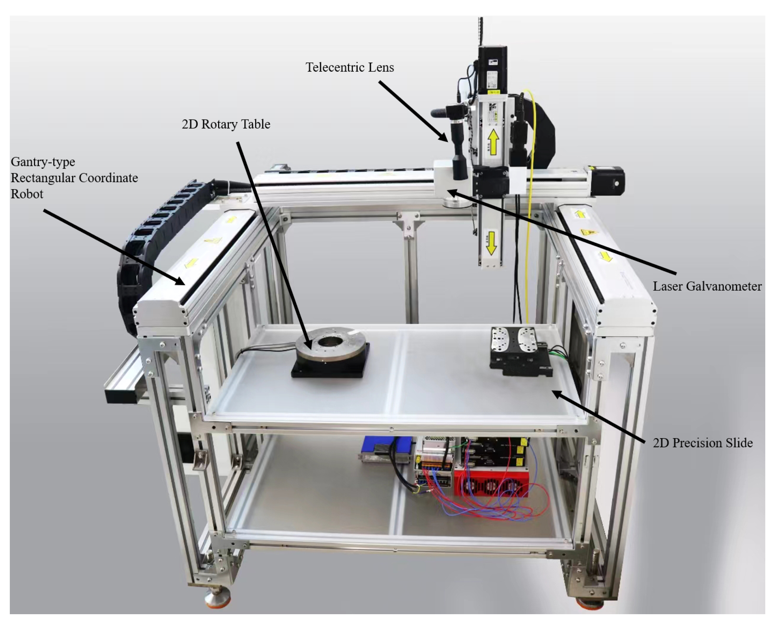
5. Experimental Validation

This section describes the tracking task and analyzes the performance of the parameter estimation method. Algorithm 1 is tested on an experimental precision-machining platform. Comparisons with other methods show its effectiveness and feasibility.

5.1. Tracking Task Description

The precision processing experimental platform shown in Figure 1 includes a gantry-type rectangular coordinate robot, an industrial camera with a telecentric lens, a laser galvanometer, a 2D rotary table, and a 2D precision slide. This system operates along the X, Y, and Z axes. The theoretical motion resolution of about 10 microns is achieved in the shaft and is suitable for processing large workpieces with accurate initial alignment. By integrating an industrial camera with a telecentric lens, stable amplification multiple can be secured at a working distance of about 25 cm, enabling high-precision measurement of the machining path plan. The laser galvanometer supports high-speed scanning and precise laser marking using a high-speed deflection mirror. The 2D rotary table provides angular positioning for polar coordinate manipulation, while the 2D precision slide enables linear motion with sub-micron precision, meeting the requirements of precision machining and accurate positioning.

The control design objective is to perform trajectory tracking; these transfer functions are described as follows:

$$G_x\left(z\right)={\displaystyle \frac{0.000691}{z-0.9324}},G_y\left(z\right)={\displaystyle \frac{0.000980}{z-0.9608}}.$$

(37)

A zero-order hold creates a discrete-time system model for analysis. The system is discretized with $T_s=0.01$ $\mathrm{s}$. Following this scheme, the continuous-time transfer function converts into a discrete-time model. The desired reference trajectory is defined as

$$r=\left\{\begin{array}{c}0.2sin(-2\pi h+\pi ),\\ 0.01h+0.02sin(-3\pi h+0.5\pi ),h\in [0,1].\end{array}\right.$$

(38)

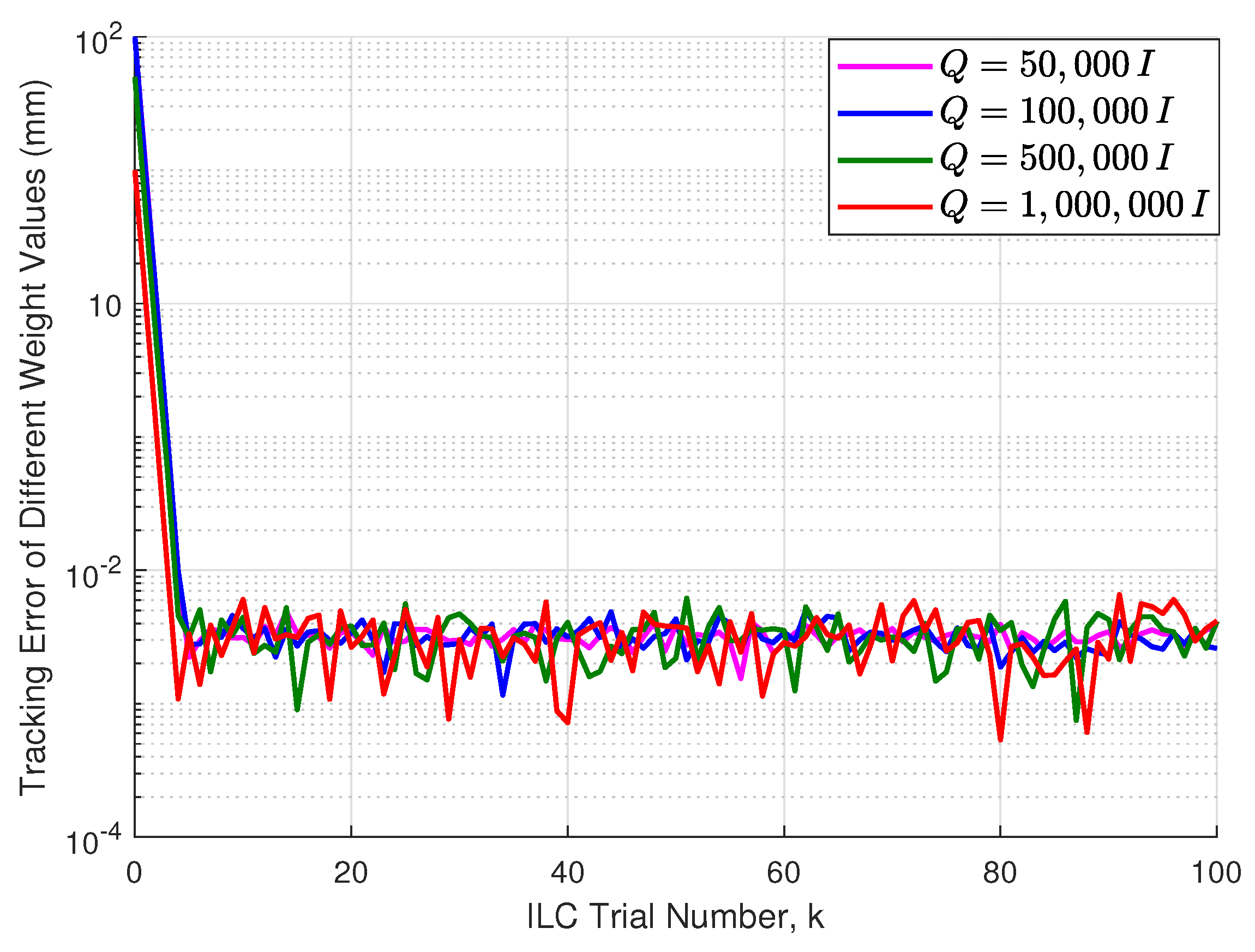
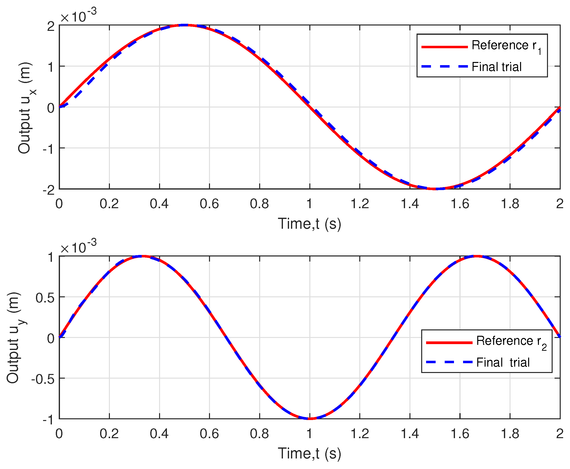
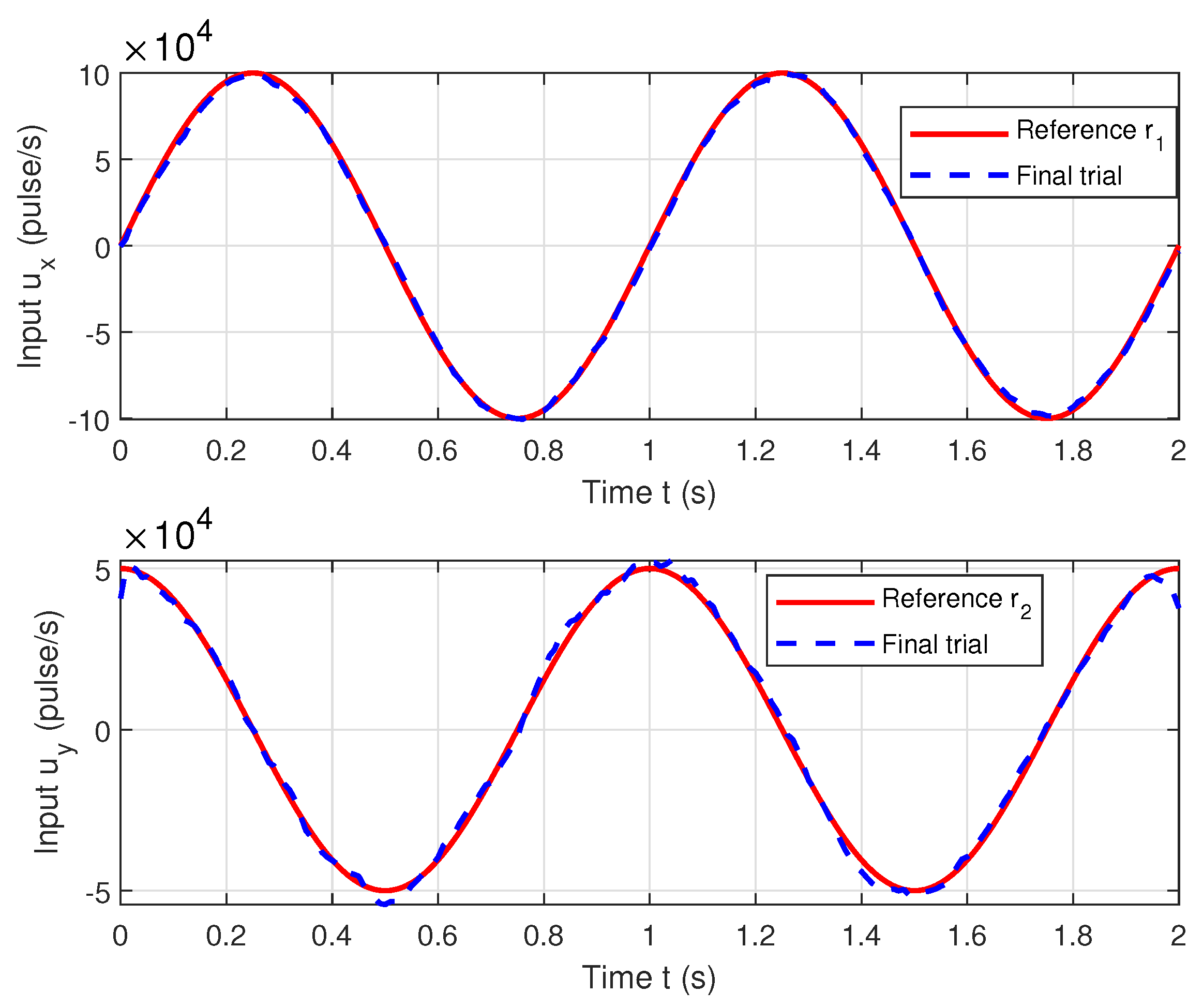
5.2. Experimental Analysis

The results presented in Figure 2 illustrate the iterative refinement of output trajectories under the proposed AKF-ILC strategy. As the number of ILC iterations increases, the tracking error exhibits a consistent reduction, demonstrating the learning capability of the algorithm. The figure depicts the output trajectories of the system across multiple trials, where the reference trajectory is represented by a red solid line, while the tracking performance at each iteration is shown by the corresponding curves. In the final trial, the output trajectory closely aligns with the reference trajectory, confirming the high tracking accuracy of the proposed approach. This outcome validates the effectiveness of the AKF-enhanced ILC strategy in dynamically adjusting to variations in system parameters and mitigating the adverse effects of uncertainties. More importantly, the results highlight the ability of the method to handle NTVSs, where the dynamics of the system evolve unpredictably over time. Such adaptability makes the proposed control framework particularly suitable for industrial applications involving complex, time-dependent uncertainties.

The selection of the weight matrix $\mathit{Q}$ plays a crucial role in determining the convergence characteristics of the ILC framework. A comparative analysis of different weight values demonstrates that increasing the magnitude of $\mathit{Q}$ significantly accelerates the reduction in the tracking error. The results indicate that a larger $\mathit{Q}$ value leads to a more rapid decline in the mean absolute error over successive iterations, thereby enhancing the learning efficiency of the iterative process. This observation underscores the importance of properly tuning the weight matrix to optimize control performance, improve convergence speed, and enhance overall system stability. The detailed comparison of these effects is depicted in Figure 3, where the influence of different $\mathit{Q}$ values on the error decay is systematically analyzed.

The variation of the mean absolute error of different control methods with respect to the number of ILC iterations $\mathrm{k}$ is shown in Figure 4. The vertical axis represents the error on a logarithmic scale, while the horizontal axis represents the ILC trial number $\mathrm{k}$. The PID control maintains a high error level, showing no significant reduction and exhibiting poor tracking accuracy. The Norm ILC method experiences a rapid error decrease in the initial stage but eventually stabilizes at the ${10}^{-2}$ magnitude, indicating moderate convergence with a relatively large residual error. The AKF-ILC method demonstrates a rapid error reduction within the first few iterations, ultimately stabilizing within the range of ${10}^{-3}$ to ${10}^{-4}$ magnitude, which is one to two orders of magnitude lower than Norm ILC. The results indicate that AKF-ILC is well suited for trajectory tracking in NTVSs, effectively reducing errors and improving tracking accuracy.

The results shown in Figure 5 demonstrate the output tracking performance of the system against the reference trajectory in the final experiment. The upper subplot illustrates the tracking accuracy of the x-axis output $u_x$ with respect to the reference trajectory $r_1$, while the lower subplot displays the y-axis output $u_y$ relative to $r_2$. The red solid line indicates the reference trajectory, and the blue dashed line represents the final output. The strong overlap between these curves within the interval of 0 to 2 s confirms the effectiveness of the proposed control strategy in accurately tracking the target trajectory. This interval corresponds to a complete trial duration in the simulation, based on a sampling time of 0.01 s.

The input signals for the system are shown in Figure 6. The upper plot presents the x-axis input $u_x$ with its reference $r_1$, while the lower plot shows the y-axis input $u_y$ with its reference $r_2$. The red solid lines denote the reference inputs, and the blue dashed lines represent the final inputs after learning. Both inputs exhibit a high degree of alignment with their references throughout the trial. This close match confirms the effectiveness of the proposed control strategy in accurately learning the required input profiles. The time interval from 0 to 2 s corresponds to one complete trial duration, defined in the simulation with a sampling time of 0.01 s.

6. Conclusions and Future Work

This paper has addressed the trajectory tracking control problem for NTVSs by developing an advanced algorithm integrating AKF with ILC. The state and observation equations of the system have been employed for mathematical modeling. Through online estimation of system parameters and real-time adaptive adjustments of noise covariance, the Kalman gain has been optimized effectively to accommodate dynamic parameter variations. Additionally, the ILC-based iterative learning law has compensated for tracking errors from preceding iterations, thereby significantly accelerating convergence and enhancing robustness to time-varying system dynamics. Experimental validations conducted on a precision machining platform have demonstrated that the proposed algorithm has achieved superior tracking accuracy and disturbance rejection compared with traditional PID and norm-optimal ILC methods. Furthermore, the low computational complexity of the algorithm and its real-time applicability have underscored the suitability of the algorithm for precision motion control systems subject to model uncertainties and parameter variations.

Future research will focus on validating the robustness of the proposed algorithm on actual precision machining systems or robotic platforms and will explore its potential extensions to systems with input–output constraints, multi-objective and cooperative control, and large-scale distributed systems. The goal will be to provide higher-performing solutions for complex industrial automation and intelligent control fields.

References

1. Zhang, G.; Zhao, X.; Wang, Q.; Ding, D.; Li, B.; Wang, G.; Xu, D. PR internal mode extended state observer-based iterative learning control for thrust ripple suppression of PMLSM drives. IEEE Trans. Power Electron. 2024, 39, 10095–10105. [Google Scholar] [CrossRef]
2. Chen, Y.; Chu, B.; Freeman, C.T. A coordinate descent approach to optimal tracking time allocation in point-to-point ILC. Mechatronics 2019, 59, 25–34. [Google Scholar] [CrossRef]
3. Chen, Y.; Freeman, C.T. Iterative learning control for piecewise arc path tracking with validation on a gantry robot manufacturing platform. ISA Trans. 2023, 139, 650–659. [Google Scholar] [CrossRef] [PubMed]
4. Ye, X.; Wen, B.; Zhang, H.; Xue, F. Leader-following consensus control of multiple nonholomomic mobile robots: An iterative learning adaptive control scheme. J. Frankl. Inst. 2022, 359, 1018–1040. [Google Scholar] [CrossRef]
5. Liu, J.; Dong, X.; Huang, D.; Yu, M. Composite Energy Function-Based Spatial Iterative Learning Control in Motion Systems. IEEE Trans. Control Syst. Technol. 2017, 26, 1834–1841. [Google Scholar] [CrossRef]
6. Hou, Z. Modified Iterative-Learning-Control-Based Ramp Metering Strategies for Freeway Traffic Control With Iteration-Dependent Factors. IEEE Trans. Intell. Transp. Syst. 2012, 13, 606–618. [Google Scholar] [CrossRef]
7. Yang, L.; Li, Y.; Huang, D.; Xia, J.; Zhou, X. Spatial iterative learning control for robotic path learning. IEEE Trans. Cybern. 2022, 52, 5789–5798. [Google Scholar] [CrossRef]
8. Liu, G.; Hou, Z. Adaptive Iterative Learning Control for Subway Trains Using Multiple-Point-Mass Dynamic Model Under Speed Constraint. IEEE Trans. Intell. Transp. Syst. 2020, 22, 1388–1400. [Google Scholar] [CrossRef]
9. Luo, D.; Wang, J.; Shen, D.; Fečkan, M. Iterative learning control for fractional-order multi-agent systems. J. Frankl. Inst. 2019, 356, 6328–6351. [Google Scholar] [CrossRef]
10. Duan, J.B.; Zhang, Z.Y. Aeroelastic Stability Analysis of Aircraft Wings with High Aspect Ratios by Transfer Function Method. Int. J. Struct. Stab. Dyn. 2018, 18, 1850150. [Google Scholar] [CrossRef]
11. Foroutan, K.; Shaterzadeh, A.; Ahmadi, H. Nonlinear static and dynamic hygrothermal buckling analysis of imperfect functionally graded porous cylindrical shells. Appl. Math. Model. 2020, 77, 539–553. [Google Scholar] [CrossRef]
12. Chen, F.; Cao, Y.; Ren, W. Distributed Average Tracking of Multiple Time-Varying Reference Signals with Bounded Derivatives. IEEE Trans. Autom. Control 2012, 57, 3169–3174. [Google Scholar] [CrossRef]
13. Huang, K.; Yuen, K.V. Online decentralized parameter estimation of structural systems using asynchronous data. Mech. Syst. Signal Process. 2020, 145, 106933. [Google Scholar] [CrossRef]
14. Chen, Y.; Li, W.; Du, Y. A novel robust adaptive Kalman filter with application to urban vehicle integrated navigation systems. Measurement 2024, 236, 114844. [Google Scholar] [CrossRef]
15. Chi, R.; Zhang, H.; Huang, B.; Hou, Z. Quantitative Data-Driven Adaptive Iterative Learning Control: From Trajectory Tracking to Point-to-Point Tracking. IEEE Trans. Cybern. 2020, 52, 4859–4873. [Google Scholar] [CrossRef]
16. Owens, D.H.; Freeman, C.T.; Van Dinh, T. Norm-Optimal Iterative Learning Control with Intermediate Point Weighting: Theory, Algorithms, and Experimental Evaluation. IEEE Trans. Control Syst. Technol. 2013, 21, 999–1007. [Google Scholar] [CrossRef]
17. Wang, L.; Huangfu, Z.; Li, R.; Wen, X.; Sun, Y.; Chen, Y. Iterative learning control with parameter estimation for non-repetitive time-varying systems. J. Frankl. Inst. 2024, 361, 1455–1466. [Google Scholar] [CrossRef]
18. Huang, Y.; Tao, H.; Chen, Y.; Rogers, E.; Paszke, W. Point-to-point iterative learning control with quantised input signal and actuator faults. Int. J. Control 2024, 97, 1361–1376. [Google Scholar] [CrossRef]
19. Guan, S.; Zhuang, Z.; Tao, H.; Chen, Y.; Stojanovic, V.; Paszke, W. Feedback-aided PD-type iterative learning control for time-varying systems with non-uniform trial lengths. Trans. Inst. Meas. Control 2023, 45, 2015–2026. [Google Scholar] [CrossRef]
20. Tao, Y.; Tao, H.; Zhuang, Z.; Stojanovic, V.; Paszke, W. Quantized iterative learning control of communication-constrained systems with encoding and decoding mechanism. Trans. Inst. Meas. Control 2024, 46, 1943–1954. [Google Scholar] [CrossRef]
21. Kim, H.; Lee, J.; Kim, J. Electromyography-signal-based muscle fatigue assessment for knee rehabilitation monitoring systems. Biomed. Eng. Lett. 2018, 8, 345–353. [Google Scholar] [CrossRef] [PubMed]
22. Jha, S.; Singh, B.; Mishra, S. Control of ILC in an autonomous AC–DC hybrid microgrid with unbalanced nonlinear AC loads. IEEE Trans. Ind. Electron. 2022, 70, 544–554. [Google Scholar] [CrossRef]
23. Chen, Y.; Chu, B.; Freeman, C.T. Iterative learning control for path-following tasks with performance optimization. IEEE Trans. Control Syst. Technol. 2021, 30, 234–246. [Google Scholar] [CrossRef]
24. Tang, Y.; Jiang, J.; Liu, J.; Yan, P.; Tao, Y.; Liu, J. A GRU and AKF-based hybrid algorithm for improving INS/GNSS navigation accuracy during GNSS outage. Remote Sens. 2022, 14, 752. [Google Scholar] [CrossRef]
25. Huangfu, Z.; Li, W.; Chen, Y.; Wang, L. ILC Coupled with Unscented Kalman Filter Strategy for Trajectory Tracking. In Proceedings of the 2024 7th International Conference on Robotics, Control and Automation Engineering (RCAE), Wuhu, China, 25–27 October 2024; pp. 598–602. [Google Scholar]
26. Cai, J.; Liu, G.; Jia, H.; Zhang, B.; Wu, R.; Fu, Y.; Xiang, W.; Mao, W.; Wang, X.; Zhang, R. A new algorithm for landslide dynamic monitoring with high temporal resolution by Kalman filter integration of multiplatform time-series InSAR processing. Int. J. Appl. Earth Obs. Geoinf. 2022, 110, 102812. [Google Scholar] [CrossRef]
27. Casey, J.A.; Kioumourtzoglou, M.A.; Padula, A.; González, D.J.; Elser, H.; Aguilera, R.; Northrop, A.J.; Tartof, S.Y.; Mayeda, E.R.; Braun, D.; et al. Measuring long-term exposure to wildfire PM2.5 in California: Time-varying inequities in environmental burden. Proc. Natl. Acad. Sci. USA 2024, 121, e2306729121. [Google Scholar] [CrossRef]
28. Ge, Q.; Hu, X.; Li, Y.; He, H.; Song, Z. A novel adaptive Kalman filter based on credibility measure. IEEE/CAA J. Autom. Sin. 2023, 10, 103–120. [Google Scholar] [CrossRef]
29. Nguyen, H.T.; Al-Sumaiti, A.S.; Vu, V.P.; Al-Durra, A.; Do, T.D. Optimal power tracking of PMSG based wind energy conversion systems by constrained direct control with fast convergence rates. Int. J. Electr. Power Energy Syst. 2020, 118, 105807. [Google Scholar] [CrossRef]
30. Chen, Y.; Chu, B.; Freeman, C.T. Iterative learning control for robotic path following with trial-varying motion profiles. IEEE/ASME Trans. Mechatron. 2022, 27, 4697–4706. [Google Scholar] [CrossRef]
31. Zhai, M.; Yang, T.; Wu, Q.; Guo, S.; Pang, R.; Sun, N. Extended Kalman Filtering-Based Nonlinear Model Predictive Control for Underactuated Systems With Multiple Constraints and Obstacle Avoidance. IEEE Trans. Cybern. 2024, 55, 369–382. [Google Scholar] [CrossRef]
32. Hoelzle, D.J.; Barton, K.L. On Spatial Iterative Learning Control via 2-D Convolution: Stability Analysis and Computational Efficiency. IEEE Trans. Control Syst. Technol. 2016, 24, 1504–1512. [Google Scholar] [CrossRef]
33. Shen, D.; Wang, Y. Survey on stochastic iterative learning control. J. Process Control 2014, 24, 64–77. [Google Scholar] [CrossRef]
34. Liang, M.; Li, J. Data-Driven Iterative Learning Security Consensus for Nonlinear Multi-Agent Systems with Fading Channels and Deception Attacks. IEEE Internet Things J. 2025. [Google Scholar] [CrossRef]
35. Li, S.; Li, X. Finite-time extended state observer-based iterative learning control for nonrepeatable nonlinear systems. Nonlinear Dyn. 2025, 1–13. [Google Scholar] [CrossRef]
36. Khodarahmi, M.; Maihami, V. A review on Kalman filter models. Arch. Comput. Methods Eng. 2023, 30, 727–747. [Google Scholar] [CrossRef]
37. Ni, X.; Revach, G.; Shlezinger, N. Adaptive KalmanNet: Data-driven Kalman filter with fast adaptation. In Proceedings of the ICASSP 2024-2024 IEEE International Conference on Acoustics, Speech and Signal Processing (ICASSP), Seoul, Republic of Korea, 14–19 April 2024; pp. 5970–5974. [Google Scholar]
38. Liu, S.; Deng, D.; Wang, S.; Luo, W.; Takyi-Aninakwa, P.; Qiao, J.; Li, S.; Jin, S.; Hu, C. Dynamic adaptive square-root unscented Kalman filter and rectangular window recursive least square method for the accurate state of charge estimation of lithium-ion batteries. J. Energy Storage 2023, 67, 107603. [Google Scholar] [CrossRef]
39. Takyi-Aninakwa, P.; Wang, S.; Zhang, H.; Xiao, Y.; Fernandez, C. A NARX network optimized with an adaptive weighted square-root cubature Kalman filter for the dynamic state of charge estimation of lithium-ion batteries. J. Energy Storage 2023, 68, 107728. [Google Scholar] [CrossRef]
40. Lavretsky, E.; Wise, K.A. Robust adaptive control. In Robust and Adaptive Control: With Aerospace Applications; Springer: London, UK, 2024; pp. 469–506. [Google Scholar]
41. Bristow, D.A.; Tharayil, M.; Alleyne, A.G. A survey of iterative learning control. IEEE Control Syst. Mag. 2006, 26, 96–114. [Google Scholar]
42. Hashemizadeh, A.; Ju, Y.; Abadi, F.Z.B. Policy design for renewable energy development based on government support: A system dynamics model. Appl. Energy 2024, 376, 124331. [Google Scholar] [CrossRef]
Figure 1. Precision machining experimental platform.
Axioms 14 00324 g001
Figure 2. The output trajectories generated by the proposed Algorithm 1 during each ILC trial.
Axioms 14 00324 g002
Figure 3. The tracking mean absolute errors of different weight values.
Axioms 14 00324 g003
Figure 4. The tracking mean absolute error comparison of PID control, normal optimal ILC, and the proposed algorithm.
Axioms 14 00324 g004
Figure 5. Comparison of final trial output and reference trajectories.
Axioms 14 00324 g005
Figure 6. Comparison of final trial input and reference trajectories.
Axioms 14 00324 g006