Article

Parameter Estimation of the Lomax Lifetime Distribution Based on Middle-Censored Data: Methodology, Applications, and Comparative Analysis

School of Mathematics and Statistics, Beijing Jiaotong University, Beijing 100044, China
*
Author to whom correspondence should be addressed.
Axioms 2025, 14(5), 330; https://doi.org/10.3390/axioms14050330 (registering DOI)
Submission received: 14 March 2025 / Revised: 11 April 2025 / Accepted: 22 April 2025 / Published: 26 April 2025
(This article belongs to the Special Issue Computational Statistics and Its Applications)

Abstract

:
The Lomax distribution has important applications in survival analysis, reliability engineering, insurance, finance, and other fields. Middle-censoring is an important censoring scheme, and data with middle-censoring will produce censoring in random intervals. This paper studies the parameter estimation of the Lomax distribution based on middle-censored data. The expectation–maximization algorithm is employed to compute the maximum likelihood estimates of the two unknown parameters of the Lomax distribution. After processing the data using the midpoint approach estimation, the parameter estimates are obtained by two computational methods: the Newton–Raphson iteration method and the fixed-point method. Moreover, the calculation methods for the asymptotic confidence intervals of the two parameters are provided, with the confidence interval coverage rate serving as one of the criteria for evaluating the estimation performance. In the Bayesian estimation aspect, the shape parameter is estimated using a Gamma prior distribution, and the Gibbs sampling method is employed for the solution. Finally, both simulation data and real data are used to compare the accuracy of the various estimation methods.

1. Introduction

The Lomax distribution, due to its flexibility in describing extreme events, is widely applied in the fields of survival analysis, reliability engineering, insurance, and finance. Middle-censoring is an important mechanism for data censoring and has extensive applications in various fields, including medical research, public health and epidemiology, economics and finance, and more. Although there is a substantial amount of literature on the parameter estimation of the Lomax distribution and middle-censored data separately, their combination has not yet been sufficiently explored. The following is a detailed elaboration on the relevant content.
In lifetime testing, data censoring often occurs, where the exact lifetime data of observed samples may only be partially available. Depending on the different types of censoring that occur in the samples, censoring types can be categorized into right censoring, left censoring, double censoring, and so on. In a study by Leiderman et al. [1], there was a double deletion model of how long it took infants to learn to complete specific tasks in the first year. Groeneboom and Wellner [2] proposed the interval-censorship model, and Schick and Yu [3] proposed the mixed case IC model.
The type of censoring we focus on in this paper is middle-censoring. Middle-censoring is a type of phenomenon in survival analysis, and this type of data was successively proposed by Huang [4] and Jammalamadaka [5] from two different perspectives. It refers to situations in practical research where continuous observation is not possible. If an event occurs in an interval not observed by researchers, only the fact that the subject experienced the event within that interval is known, but not the exact time of occurrence. In the middle-censoring scheme, for n sample units, the lifetimes of the sample units are denoted as T 1 , T 2 , , T n . For the i-th unit (i = 1, 2, …, n), there exists a random censoring interval [ L i , R i ] , which follows an unknown bivariate distribution and is independent of the lifetime. The exact failure time T i of the i-th unit can only be observed if T i [ L i , R i ] . Otherwise, only the censored interval [ L i , R i ] is observed.
Many studies have been conducted on middle-censoring for parametric models. Jammalamadaka and Iyer [6] considered the approximate self-consistency of middle-censored data. Yu, Wong and Li [7] established strong consistency, asymptotic normality, and asymptotic efficiency of the self-consistent estimator and the generalized MLE with middle-censored data. Srikanth K. Iyer [8] studied the maximum likelihood estimation of exponential distributions with middle-censored data and investigated its consistency and asymptotic normality properties. Bennett et al. [9] provided a proof that the EM algorithm converges in such cases. Wang et al. [10] studied the bivariate Weibull distribution and considered the statistical analysis of related competing risks models, obtaining the maximum likelihood estimation (MLE), midpoint approximation (MPA) estimation, and approximate confidence intervals (ACI) for the unknown parameters. Jammalamadaka et al. [11] analyzed discrete lifetime data that follow a geometric distribution that is subject to middle-censoring.
The Lomax distribution, often referred to as the second type of Pareto distribution, was first proposed by K.S. Lomax [12] in 1954. It plays an important role in the analysis of lifetime data in medicine, biological sciences, and engineering. In recent years, many articles have studied the extensions of this distribution and its related statistical properties. For example, Lun [13] conducted research and pointed out the connection between the Lomax lifetime distribution and the exponential distribution under specific conditions. Aljohani et al. [14] investigated the statistical inference of the stress–strength reliability R = P ( X > Y ) of the Lomax distribution under accelerated life testing, using both classical and Bayesian methods for point estimation of R. Alsuhabi et al. [15] extended the Lomax lifetime distribution by proposing a new continuous lifetime model with four parameters, estimating the model parameters using classical methods (e.g., maximum likelihood estimation (MLE) and maximum product of spacings) and non-classical methods (e.g., Bayesian analysis).
Many researchers have studied the estimation methods for the parameters of the Lomax distribution under censoring. Cramer et al. [16] discussed the competing risks model of the Lomax distribution under progressive Type-II censoring, establishing the maximum likelihood estimation of the distribution parameters. Alfaer et al. [17] studied the Lomax lifetime distribution under a balanced joint progressive Type-I censoring scheme, providing point estimates and asymptotic confidence intervals for the model parameters using maximum likelihood estimation. Bayesian estimates and related credible intervals were obtained using MCMC techniques under independent Gamma priors. El-Sherpieny [18] studied the Power Lomax distribution under progressive Type-II hybrid censoring. The authors discussed parameter estimation for this distribution using maximum likelihood estimation (MLE) and the maximum product spacing method. Hasaballah et al. [19] conducted research on parameter estimation for the Lomax lifetime distribution under censored data, employing both Bayesian and non-Bayesian methods to estimate the parameters.
There is an extensive body of research on the Lomax distribution and middle-censoring, and the existing research results are shown in Figure 1.
However, there has been no research to date that establishes a connection between these two concepts. Therefore, this paper aims to address this issue by studying parameter estimation of the Lomax distribution based on middle-censored data and by comparing and analyzing different estimation methods.
In Section 2 of our paper, we introduce the Lomax distribution as a continuous probability distribution and conduct modeling for middle-censored data. We provide a detailed expression for the maximum likelihood estimation under middle-censoring for the Lomax distribution and discuss its properties, which are crucial for the subsequent estimation methods.
In Section 3, we delve into frequentist methods for parameter estimation. We propose the EM algorithm to address the maximum likelihood estimation (MLE) problem for the two unknown parameters of the Lomax distribution. We also provide two alternative solutions for midpoint approach estimation (MPA). Additionally, we calculate the approximate confidence intervals for these parameters, which are necessary for statistical inference.
In Section 4, we explore Bayesian estimation methods, which offer a different perspective on parameter estimation compared to frequentist methods. We use a Gamma distribution as the prior for the shape parameter of the Lomax distribution and apply Bayesian techniques to estimate the parameters. This approach allows us to incorporate prior knowledge and provides a complete posterior distribution for the parameters.
In Section 5, we present the results of simulation experiments and experiments with real datasets. These experiments are designed to assess the accuracy of the various parameter estimation methods developed in the previous sections and to demonstrate their practical utility in real-life scenarios.
Finally, we summarize the main findings of this paper and discuss the significance of this research. In addition, we propose directions for future research and potential solutions.

2. Model Description

2.1. Lomax Distribution

The exponential distribution, commonly encountered in daily life, has a thin tail and is suitable for describing memoryless random events. In contrast, the Lomax distribution is a heavy-tailed distribution, making it more appropriate for modeling data with heavy-tailed characteristics and for describing extreme events. Additionally, compared with the Weibull distribution, whose shape parameter can control the thickness of the tail, the Lomax distribution may be more suitable for describing certain specific types of heavy-tailed data. In practical applications, the Lomax distribution is widely used in areas such as survival analysis (e.g., the lifetime of power transformers), wealth distribution, and queuing service times. Suppose the random variable T follows Lomax distribution, then its probability density function (PDF) and cumulative distribution function (CDF) are given by the Functions (1) and (2).
f t = θ λ 1 + t λ θ + 1 , t > 0 ,
F t = 1 1 + t λ θ , t > 0 .
where λ is called the scale parameter, θ is called the shape parameter, λ > 0, θ > 0.
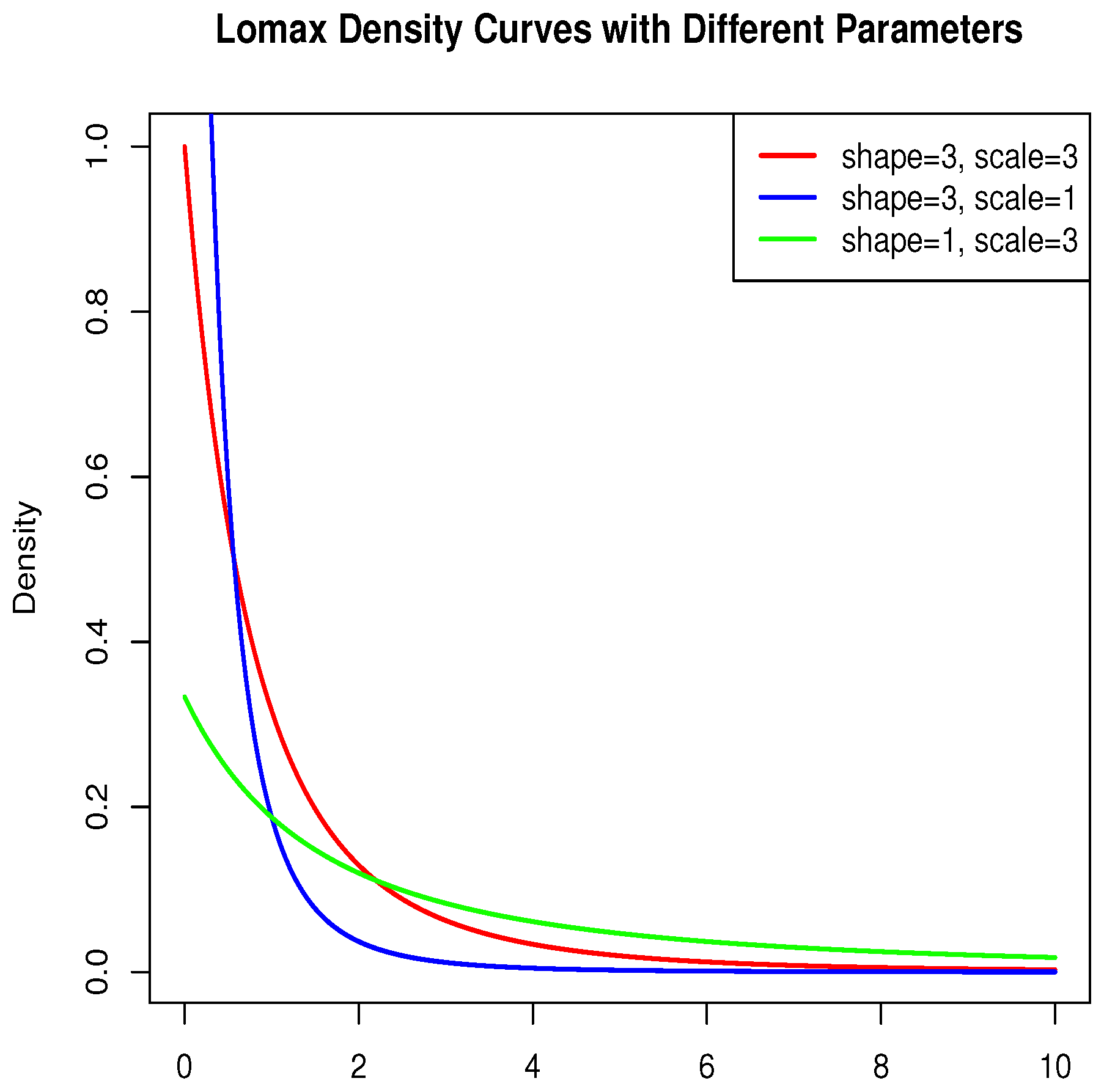
The probability density functions of the Lomax distribution with different parameters are shown in Figure 2.
The Lomax distribution can be regarded as a heavy-tailed version of the exponential distribution. While the tail of the exponential distribution decays exponentially, the tail of the Lomax distribution decays according to a power law, specifically ( x + λ ) ( θ + 1 ) . When θ is small, the Lomax distribution has a heavier tail, making it more suitable for describing extreme events. Compared to the exponential distribution, the shape parameter θ and the scale parameter λ of the Lomax distribution provide sufficient flexibility to adapt to different types of data distributions. Therefore, the Lomax distribution has broader applications than the exponential distribution in some cases.

2.2. The Middle-Censoring Model of Lomax

The type of censoring we focus on in this paper is middle-censoring. If a data point falls within a random interval and is not observable, middle-censoring occurs. The middle-censoring scheme can be described as follows.
From the Figure 3, we can see the schematic diagram of the middle-censored data type. For some data, we can only observe the interval form and cannot observe the exact values.
For middle-censored data, there are two modeling approaches. One, proposed by Huang [4], specifically describes that observers selectively observe at certain times. When the lifetime data ends at the observation point, the data is observed; when the end occurs between two observation times, the data can only be recorded as an interval with the two observation times as its endpoints. The other, proposed by Jammalamadaka [5], specifically describes that during the continuous observation of data, there will be intervals that are not observed. When the lifetime data ends within this interval, the data will not be observable. The two think from different angles but the final effect is the same, both are descriptions of middle-censored data. This paper adopts the second modeling approach for middle-censored data.
Assume that n items are tested, and the lifetimes of these items are T 1 , …, T n . For item i, there exists a random censored interval [ L i , R i ] , which follows some unknown bivariate distribution. T i can be observed only when T i [ L i , R i ] , otherwise it cannot be observed. Suppose δ i = I ( T i [ L i , R i ] ) , where I (·) denotes the indicator function. Therefore, when δ i = 1 , the observed results are not censored, and we observe the actual value t i = T i . In this case, we did not observe [ L i , R i ] . On the other hand, when δ i = 0 , we only observe the truncated interval [ L i , R i ] . For item i, we observe the following Formula (3):
t i , 1 i f T i L i , R i L i , R i , 0 o t h e r w i s e .
In this section, the distribution of the two ends of the censored interval is unknown. In the subsequent parameter estimation test, the exponential distribution with different mean values is used to generate the two ends of the censored data to manually censor the data.

3. Frequentist Estimation

In this section, we use the traditional frequency method and the approximation method to represent the point and interval estimation of the unknown parameters.

3.1. Maximum Likelihood Estimation

Assuming that the number of actual observed data size is n 1 , the number of middle-censored sample is n 2 , and the total number of sample is n. Let t i be the observed data point, and L i and R i be the endpoints of the observed middle-censoring interval.
t 1 , 1 , t 2 , 1 , , t n 1 , 1 , L n 1 + 1 , R n 1 + 1 , 0 , L n 1 + 2 , R n 1 + 2 , 0 , , L n 1 + n 2 , R n 1 + n 2 , 0 .
The likelihood function of the shape parameter θ and the scale parameter λ based on middle-censored data of the Lomax life distribution [20] is
L θ , λ = i = 1 n 1 f t i i = n 1 + 1 n 1 + n 2 F R i F L i .
Substituting into Functions (1) and (2), we can obtain Function (6).
L θ , λ = θ n 1 λ n 1 i = 1 n 1 1 + t i λ θ + 1 i = n 1 + 1 n 1 + n 2 1 + t i λ θ 1 + t i λ θ .
Taking the logarithm of Function (6), we obtain the log-likelihood function.
ln L θ , λ = n 1 ln θ n 1 ln λ θ + 1 i = 1 n 1 ln 1 + t i λ + i = n 1 + 1 n 1 + n 2 ln 1 + L i λ θ 1 + R i λ θ .
By differentiating Function (7) with respect to the two parameters, we obtain Functions (8) and (9).
ln L θ , λ θ = n 1 θ i = 1 n 1 ln 1 + t i λ + i = n 1 + 1 n 1 + n 2 λ + L i θ ln 1 + R i λ λ + R i θ ln 1 + L i λ λ + R i θ λ + L i θ .
ln L θ , λ λ = n 1 λ + θ + 1 i = 1 n 1 t i λ 2 + λ t i + i = n 1 + 1 n 1 + n 2 θ λ R i λ + L i θ + 1 L i λ + R i θ + 1 λ + R i θ + 1 λ + L i λ + L i θ + 1 λ + R i .
Equation (10) is obtained by setting the two functions to zero and joining them.
n 1 θ i = 1 n 1 ln 1 + t i λ + i = n 1 + 1 n 1 + n 2 λ + L i θ ln 1 + R i λ λ + R i θ ln 1 + L i λ λ + R i θ λ + L i θ = 0 n 1 λ + 1 + θ i = 1 n 1 t i λ 2 + λ t i + i = n 1 + 1 n 1 + n 2 θ λ R i λ + L i θ + 1 L i λ + R i θ + 1 λ + R i θ + 1 λ + L i λ + L i θ + 1 λ + R i = 0 .
The strong consistency, asymptotic normality, and asymptotic efficiency of the maximum likelihood estimation under middle-censoring have been proven [7]. When the data are complete, we can directly solve for the shape parameter θ and the scale parameter λ using this expression, and the existence and uniqueness of the solution can be proven [21]. MLE with middle-censored data also possesses similar properties, but due to the presence of middle-censoring data, it is not feasible to directly derive the maximum likelihood estimates of the parameters. To solve this problem, we will use the EM algorithm to process the missing data.

3.2. Expectation–Maximization Algorithm

The expectation–maximization (EM) algorithm [22] is an iterative optimization algorithm commonly used for models with latent variables or missing data. In the parameter estimation of middle-censored data, the EM algorithm has significant advantages, as it can effectively handle missing data issues and gradually improve the accuracy of parameter estimation through iterative optimization. In most cases, the algorithm converges to a local optimal solution [23]. For many practical problems, the local optimal solution is sufficiently good. Its simplicity, flexibility, and numerical stability make it the preferred method for many practical problems. In particular, for exponential family distributions (such as the Lomax distribution) [22], the E-step and M-step calculations usually have closed-form solutions.
The core idea of the EM algorithm is to gradually improve the estimation of parameters by constructing an expectation step (E-step) and a maximization step (M-step). At the same time, let t i * ( i = n 1 + 1 , n 1 + 2 , , n ) be the failure time in the interval [ L i , R i ] at iteration step k, then the complete data can be obtained.
t 1 , 1 , t 2 , 1 , , t n 1 , 1 , t n 1 + 1 * , 0 , , t n 1 + n 2 * , 0 .
By completing the complete data, the likelihood function can be obtained as Function (12).
L c θ , λ = i = 1 n 1 f t i i = n 1 + 1 n 1 + n 2 f t i * .
The log-likelihood function is
ln L c θ , λ = n ln θ n ln λ θ + 1 i = 1 n 1 ln 1 + t i λ θ + 1 i = n 1 + 1 n 1 + n 2 ln 1 + t i * λ .
The expected values of the shape parameter and scale parameter are expressed as Equation (14) and Equation (15), respectively, where f ( t ; θ , λ ) and F ( t ; θ , λ ) represent the probability density function and cumulative distribution function of the Lomax distribution under specific parameters.
E θ , λ ln 1 + T i λ T i L i , R i = L i R i ln 1 + t λ f t ; θ , λ d t F R i ; θ , λ F L i ; θ , λ ,
E θ , λ T i λ 2 + λ T i T i L i , R i = L i R i t λ 2 + λ T i f t ; θ , λ d t F R i ; θ , λ F L i ; θ , λ .
The EM algorithm is frequently used to handle parameter estimation problems under middle-censored data [24], and the corresponding algorithm steps are as follows (Algorithm 1):
Algorithm 1: EM Algorithm for parameter estimation.
1:
Initialize the parameter values λ ( 0 ) and θ ( 0 ) using an exponential distribution, and set the tolerance threshold ε = 0.05 .
2:
E-step: During the k-th iteration, calculate the expected values.
E 1 i ( k ) = E θ ( k 1 ) , λ ( k 1 ) ln 1 + T i λ T i ( L i , R i ) E 2 i ( k ) = E θ ( k 1 ) , λ ( k 1 ) ln 1 + T i λ T i = t i E 3 i ( k ) = E θ ( k 1 ) , λ ( k 1 ) T i λ 2 + λ T i T i ( L i , R i ) E 4 i ( k ) = E θ ( k 1 ) , λ ( k 1 ) T i λ 2 + λ T i T i = t i
3:
M-step: Update the parameter estimates by maximizing the likelihood function L c ( θ , λ ) based on the complete data.
θ ( k ) = n i = 1 n 1 E 1 i ( k ) + i = n 1 + 1 n 1 + n 2 E 2 i ( k ) λ ( k ) = n ( θ ( k ) + 1 ) i = 1 n 1 E 3 i ( k ) + i = n 1 + 1 n 1 + n 2 E 4 i ( k )
4:
Convergence Check: If the following conditions are met, stop the iteration; otherwise, return to Step 2.
| θ ( k ) θ ( k 1 ) | < ε | λ ( k ) λ ( k 1 ) | < ε
The value of ε in the algorithm needs to be adjusted according to the actual situation. When higher precision for estimation is required, a smaller ε can be chosen. When higher computational efficiency is desired, a smaller ε can also be chosen.
By iterating through the above EM algorithm, the estimated values of λ and θ can be obtained.

3.3. Midpoint Approach Estimation

Besides the EM estimation, the midpoint approach estimation (MPA) is also a method used for handling censored data [25], which is especially common in survival analysis and reliability engineering. This method replaces the censored data with the midpoint of the censored interval, thereby performing parameter estimation.
For censored data, we use the average of the two endpoints of the censored interval to replace the censored data.
t i ^ = L i + R i 2 .
t 1 , 1 , t 2 , 1 , , t n 1 , 1 , t n 1 + 1 ^ , 0 , , t n 1 + n 2 ^ , 0 .
After obtaining the complete data using the midpoint estimation method, the estimates of the shape and scale parameters can be obtained by solving the equations using the Newton–Raphson iteration method and the fixed-point method. For the complete data, the likelihood function is given by Function (18).
L M θ , λ = i = 1 n 1 f t i i = n 1 + 1 n 1 + n 2 f t i ^ = i = 1 n 1 θ λ θ t i + λ θ + 1 i = n 1 + 1 n 1 + n 2 θ λ θ t i ^ + λ θ + 1 .

3.3.1. The Newton–Raphson Iteration Method for Solving Under the MPA Estimation

Since the censored interval data have been imputed by the midpoint values of the intervals, the statistical software can directly compute the solutions for the two parameters. Therefore, the Newton–Raphson iteration method can be employed to obtain the estimates of the scale parameter and the shape parameter.
The negative log-likelihood function is given by Function (19).
n e g _ l o g _ l i k e l i h o o d = ln L M θ , λ = i = 1 n 1 ln θ λ θ t i + λ θ + 1 + i = n 1 + 1 n 1 + n 2 ln θ λ θ t i ^ + λ θ + 1 .
Using R program (version 4.3.2) (All the codes in the text are run with this device. The device models are as follows: LAPTOP-90NAADHP, equipped with an Intel(R) Core(TM) i7-10510U CPU running at 1.80 GHz with a boost speed of 2.30 GHz. It has 16.0 GB of RAM, with 15.8 GB available. The device ID is B0B39209-7A3F-4006-81CE-AB49F27A02E1, and the product ID is 00342-35692-61862-AAOEM. The system is a 64-bit operating system based on an x64 processor.) for calculation: Select appropriate initial values λ 0 and θ 0 , we can utilize the general optimization function optim to find the minimum of the negative log-likelihood function, thereby obtaining the estimates of the shape and scale parameters.

3.3.2. The Fixed-Point Method for Solving Under the MPA Estimation

After taking the logarithm of the likelihood Function (18) for the complete data and differentiating with respect to the two parameters, the resulting system of equations, where the derivatives are set to zero, is given as Equation (20).
n θ i = 1 n 1 ln 1 + t i λ + i = n 1 + 1 n 1 + n 2 ln 1 + t i λ = 0 n λ + 1 + θ i = 1 n 1 t i λ 2 + λ t i + i = n 1 + 1 n 1 + n 2 t i ^ λ 2 + λ t i ^ = 0 .
The expression for the shape parameter θ in terms of the scale parameter λ is obtained through transformation by Equation (20).
θ λ = n i = 1 n 1 ln 1 + t i λ + i = n 1 + 1 n 1 + n 2 ln 1 + t i ^ λ .
Substituting Function (21) into Equation (20) results in
n λ 1 + θ λ i = 1 n 1 t i λ 2 + λ t i + i = n 1 + 1 n 1 + n 2 t i ^ λ 2 + λ t i ^ = 0 .
To solve Equation (22), we use the fixed-point method. First, we define the function g ( λ ) as
g λ = 1 n 1 + n i = 1 n 1 Q i + i = n 1 + 1 n 1 + n 2 Q ^ i i = 1 n 1 P i + i = n 1 + 1 n 1 + n 2 P ^ i .
The symbols in this equation are defined as
Q i = ln 1 + t i λ , Q ^ i = ln 1 + t i ^ λ , P i = t i 1 + t i λ , P i ^ = t i ^ 1 + t i ^ λ .
Select an appropriate initial value λ 0 , and use the fixed-point iteration method in the R program (version 4.3.2) to solve the equation iteratively. This will yield a proper solution λ . Substituting λ into Function (21) allows us to obtain the estimate of θ .

3.4. The Estimation of Asymptotic Confidence Interval

Censored data, such as the introduction of missing data in the middle, may lead to biased parameter estimates. The censoring mechanism can affect the sample distribution, making it impossible to directly use standard asymptotic theory because the sample distribution is no longer a simple known distribution. Meanwhile, with censored data, increasing the sample size does not necessarily result in more reliable estimates, especially when the degree of censoring is high, as the sample may fail to reflect the true characteristics of the population.
The asymptotic confidence interval (ACI) is a statistical method used for estimating the confidence interval of a parameter. Unlike the classical confidence interval, the ACI is derived based on the properties when the sample size approaches infinity.
For the parameters θ and λ , it is impossible to obtain an exact confidence interval. Therefore, we use the asymptotic properties of maximum likelihood estimators to construct the ACI [26].
The observed Fisher information matrix for parameters θ and λ is represented as
I λ , θ = I 11 I 12 I 21 I 22 ,
I 11 = 2 ln L θ , λ λ 2 , I 22 = 2 ln L θ , λ θ 2 ,
I 12 = I 21 = 2 ln L θ , λ λ θ .
The logarithm of the likelihood is ln L ( θ , λ ) . We calculate I 11 , I 12 , I 21 , and I 22 , and substitute the estimated values of λ ^ and θ ^ into the calculation formula for the Fisher matrix. The inverse of the matrix yields Function (28).
W λ , θ = I 11 I 12 I 21 I 22 1 | λ = λ ^ , θ = θ ^ = W 11 ^ W 12 ^ W 21 ^ W 22 ^ .
Through the asymptotic distribution properties of the likelihood function, we know that λ λ ^ / W 11 ^ , θ θ ^ W 22 ^ both follow a standard normal distribution. Under a confidence level of γ , the asymptotic confidence intervals for the parameters θ and λ can be obtained.
λ ^ Z γ 2 W 11 ^ , λ ^ + Z γ 2 W 11 ^ ,
θ ^ Z γ 2 W 22 ^ , θ ^ + Z γ 2 W 22 ^ .

4. Bayes Estimation

4.1. The Posterior Distribution of the Parameters of the Lomax Distribution Under Middle-Censoring

When the scale parameter λ is known, we choose the Gamma distribution with parameters a and b as the prior distribution for the shape parameter θ  [27], and denote it as  π ( θ ) .
π ( θ ) = b a Γ ( a ) θ a 1 e b θ .
Since the Gamma distribution is the conjugate prior for the shape parameter of the Lomax distribution, it has desirable properties when selected as the prior distribution. The proof that the Gamma distribution is the conjugate prior for the shape parameter of the Lomax distribution has been included in the Appendix A to ensure the rigor of the paper.
Suppose the experimental data with middle-censoring are denoted as data; then, the likelihood function of data can be represented as p ( data θ ) , and the joint distribution of data and θ is h ( data , θ ) . By integrating h ( data , θ ) over the parameter space Θ , we can obtain the marginal density of data, denoted as m ( data ) .
data = t 1 , 1 , t 2 , 1 , , t n 1 , 1 , L n 1 + 1 , R n 1 + 1 , 0 , L n 1 + 2 , R n 1 + 2 , 0 , , L n 1 + n 2 , R n 1 + n 2 , 0 .
p ( d a t a | θ ) = L ( θ , λ ) = θ n 1 λ n 1 i = 1 n 1 1 + t i λ θ + 1 i = n 1 + 1 n 1 + n 2 1 + t i λ θ 1 + t i λ θ .
h ( d a t a , θ ) = p ( d a t a | θ ) π ( θ ) = θ n 1 λ n 1 i = 1 n 1 1 + t i λ θ + 1 i = n 1 + 1 n 1 + n 2 1 + t i λ θ 1 + t i λ θ b a Γ ( a ) θ a 1 e b θ .
m d a t a = Θ h d a t a , θ d θ = Θ p d a t a | θ π θ d θ .
From Functions (34) and (35), we can derive the posterior distribution of the parameter θ given data.
π θ | d a t a = h d a t a , θ m d a t a θ n i = 1 n 1 1 + t i λ θ θ a 1 e b θ i = n 1 + 1 n 1 + n 2 1 + t i λ θ 1 + t i λ θ .
Using the absolute error loss function, we can obtain the Bayesian estimate of the shape parameter θ .
MSE = 1 M i = 1 M ( θ θ ^ i ) 2 .

4.2. The Bayesian Estimation of the Shape Parameter Based on Gibbs Sampling When the Scale Parameter Is Known

Directly solving the posterior distribution by integration poses some difficulties. Therefore, we resort to Gibbs sampling for the relevant computations of the posterior distribution. Gibbs sampling is a sampling technique within the Markov Chain Monte Carlo methods and is widely used in Bayesian inference. It generates approximate samples from a target distribution by iteratively sampling from conditional distributions [28].
To utilize Gibbs sampling, we first need to establish the condition that, when the data are complete and the scale parameter is known, the conditional posterior density of the shape parameter follows a Gamma distribution. Let the complete data be denoted as data * .
Theorem 1. 
When the data are complete and the scale parameters are known, the posterior condition density of the shape parameters is Gamma distribution.
Proof. 
Through the likelihood function of the Lomax distribution, we can obtain the conditional posterior density of the shape parameter when the data are complete.    □
π θ | d a t a * θ n i = 1 n 1 + t i λ θ θ a 1 e b θ .
Thus, when the scale parameter is known, the conditional posterior distribution of the shape parameter is
G a m m a n + a , b + i = 1 n ln 1 + t i λ .
Therefore, the conclusion is proved. The steps to obtain the shape parameter using Gibbs sampling when the scale parameter is known are shown in Algorithm 2.
Algorithm 2: Gibbs sampling method for estimating shape parameter θ .
1:
Determine the initial value of the shape parameter θ 0 . Define the number of Gibbs sampling iterations as M and the number of initial samples to be discarded as Q.
2:
In the k-th iteration, the missing data in the interval are replaced by conditional expectations, and the replaced values are denoted as t i k # , for i = n 1 + 1 , n 1 + 2 , , n 1 + n 2 .
t i k # = E ( T | T ( L i , R i ) ; λ , θ k 1 ) = L i R i T f ( T ; λ , θ k 1 ) d T F ( R i ; λ , θ k 1 ) F ( L i ; λ , θ k 1 )
3:
Substitute the imputed data into the distribution, and then randomly draw a sample from the distribution to obtain θ k .
G a m m a n + a , b + i = 1 n 1 ln 1 + t i λ + i = n 1 + 1 n 1 + n 2 ln 1 + t i k # λ .
4:
Repeat Steps 2 and 3 M times to obtain M posterior conditional distribution-related sample data θ k . The estimate of the shape parameter θ based on the sum of squared loss function is
θ ^ bayes = k = Q + 1 M Q θ k M Q .
By following the above Gibbs sampling steps, the Bayesian estimate of the shape parameter can be obtained through programming when the scale parameter is known.

5. Simulation Experiments and Real Data Analysis

5.1. Analysis of Simulation Experiments

5.1.1. Analysis of the Solution Methods for MPA Estimation

Using the R program (version 4.3.2), we generate data with three different sets of parameters, where λ is the scale parameter and θ is the shape parameter. For each data point, censoring intervals are randomly generated using an exponential distribution with different parameters to determine whether the data point is censored. We then perform parameter estimation using the aforementioned methods on the middle-censored data.
The estimated parameters are compared with the true parameters used for data generation. The accuracy of the parameter estimates is evaluated using bias and mean absolute error (MAE). The relevant formulas are as follows:
L M A E = 1 M i = 1 M λ λ i ^ , L B i a s = 1 M i = 1 M λ λ i ^ , T M A E = 1 M i = 1 M θ θ i ^ , T B i a s = 1 M i = 1 M θ θ i ^ .
We also calculate the coverage probability of the asymptotic confidence intervals for the parameter estimates to assess the reliability of these intervals in containing the true parameters. The coverage probability is defined as the proportion of intervals that include the true parameter value.
I A C I λ = 1 , λ λ ^ Z γ 2 W 11 ^ , λ ^ + Z γ 2 W 11 ^ 0 , λ λ ^ Z γ 2 W 11 ^ , λ ^ + Z γ 2 W 11 ^ ,
I A C I θ = 1 , θ θ ^ Z γ 2 W 22 ^ , θ ^ + Z γ 2 W 22 ^ 0 , θ θ ^ Z γ 2 W 22 ^ , θ ^ + Z γ 2 W 22 ^ .
A C θ = E I A C I θ , A C λ = E I A C I λ .
In subsequent simulations and experiments with real data, the significance level γ of the confidence interval was set to 0.05.
We test the selection of initial values for the simulation experiments and find that the choice of initial values does not affect the convergence of these three estimation methods, which still provide good estimation results. For the fixed-point estimation method, the iterative initial values of the scale parameters are generated using an exponential distribution with an average of 1. For Newton–Raphson algorithm, the iterative initial values of shape parameters are generated using an exponential distribution with a mean of 1, and the iterative initial values of scale parameters are generated using an exponential distribution with a mean of 1.
During the estimation process, the nature of randomly generated middle-censored data may be poor, leading to a compromise in the convergence of the algorithm, resulting in a significant discrepancy between the simulated estimated parameters and the actual set parameters. This can affect the assessment of the accuracy of the estimation method. Therefore, for the parameter estimation results in the looped simulation process, the following outlier removal scheme is adopted: If a data point exceeds the range of P 1 1.5 × I Q R or P 2 + 1.5 × I Q R , it is considered an outlier and is removed before assessing the accuracy of the estimation results. P 1 represents the first quartile of the estimated parameter results from all iterations, P 2 represents the third quartile of the estimated parameter results from all iterations, and IQR = P 2 P 1 . In the simulation results table, we use OR to denote Outlier Ratio, which means the proportion of simulation experiments where the estimation results are outliers out of the total number of experiments during the iterative simulation process.
By comparing the Newton–Raphson iterative method and the fixed-point estimation method, we obtain the accuracy and efficiency of the two methods under different parameter combinations. The results are shown in the following Table 1 and Table 2.
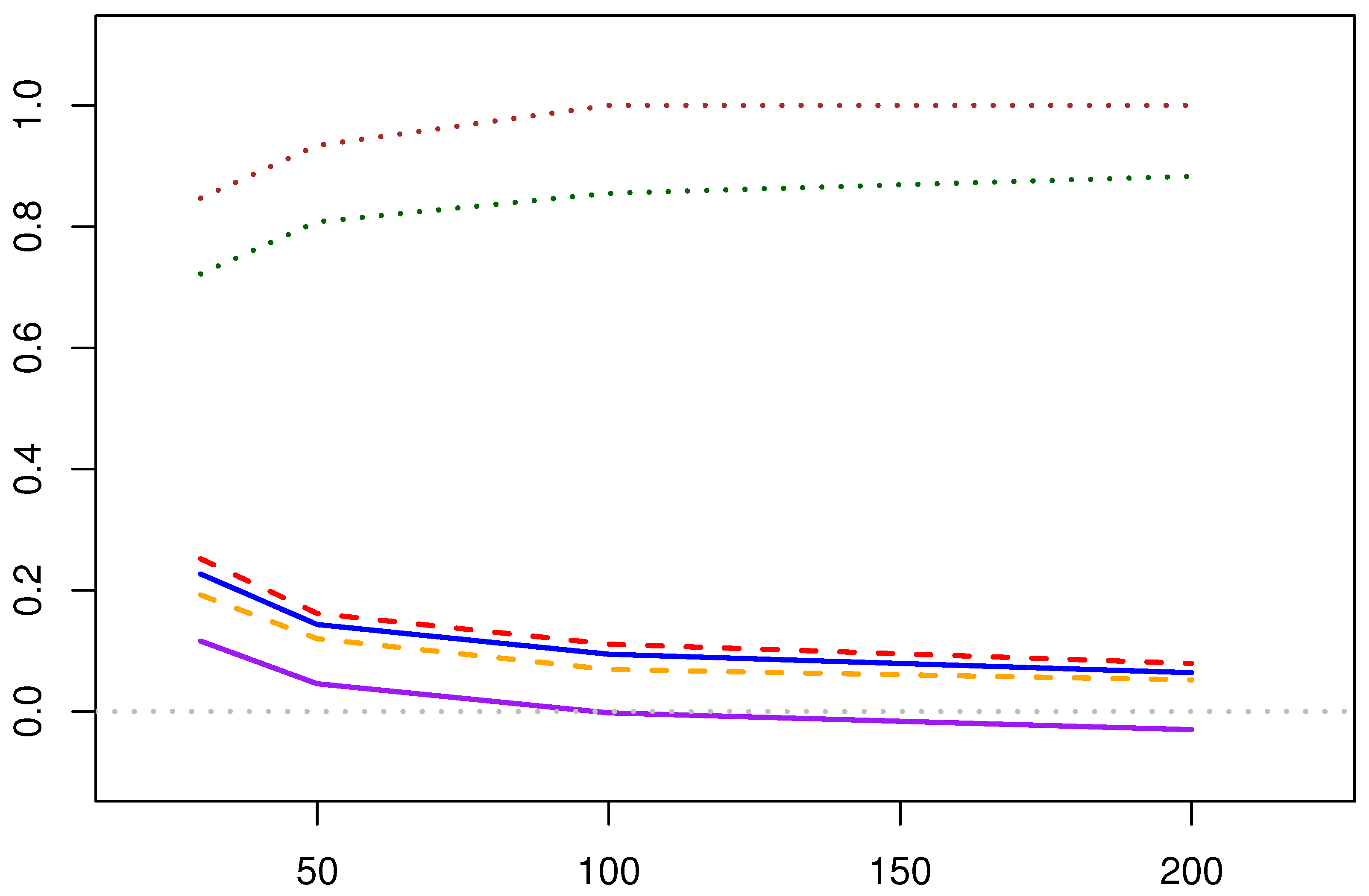
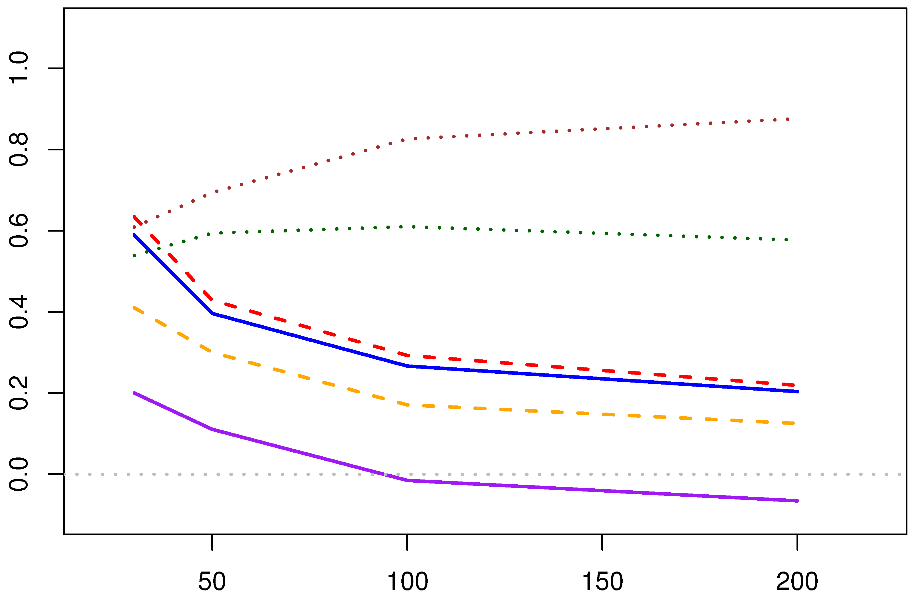
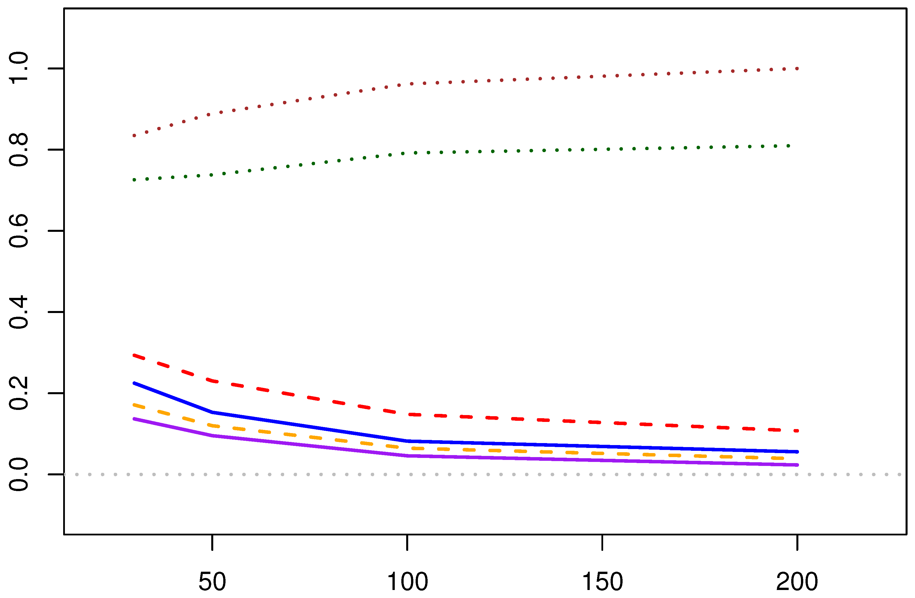
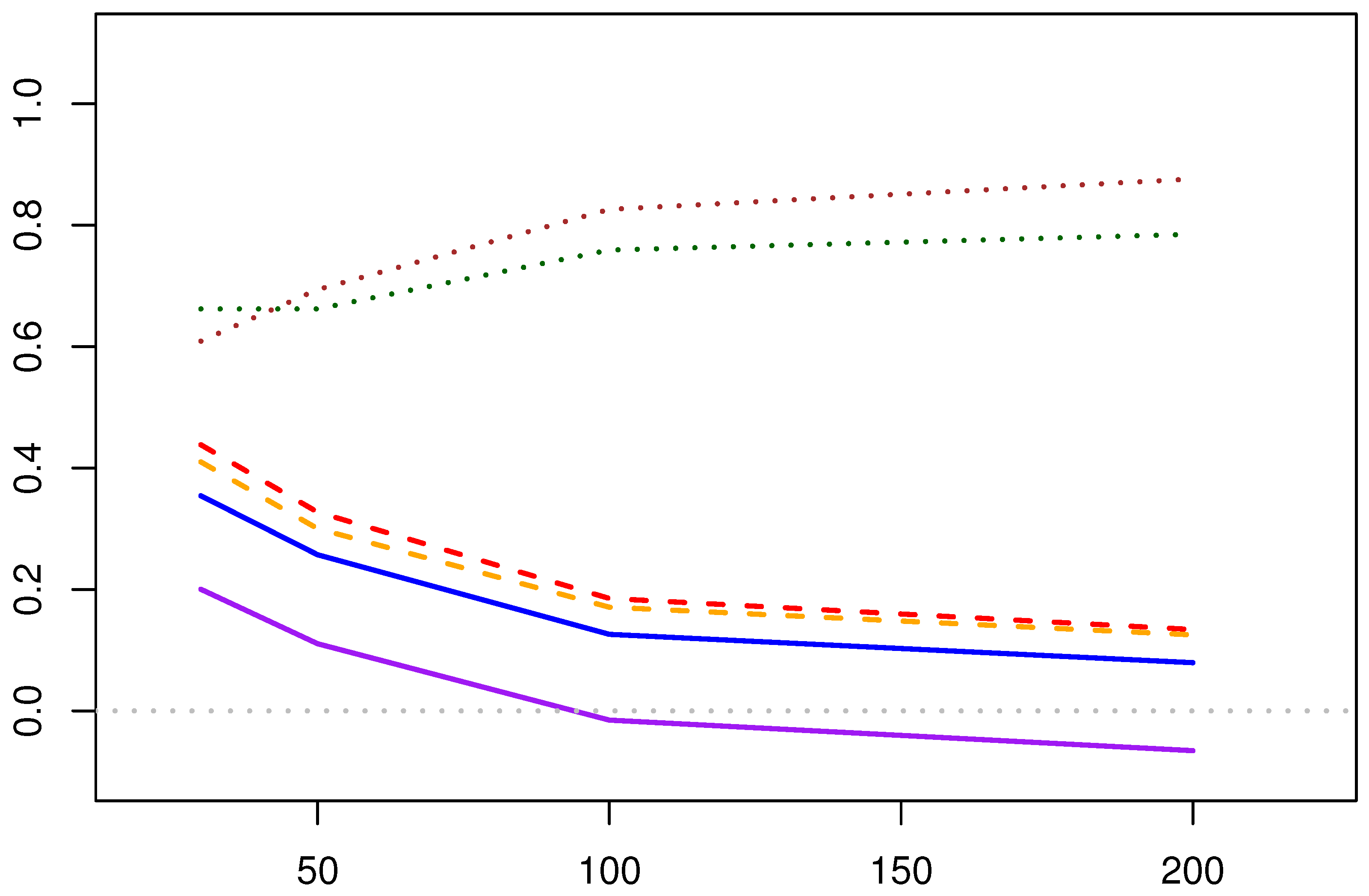
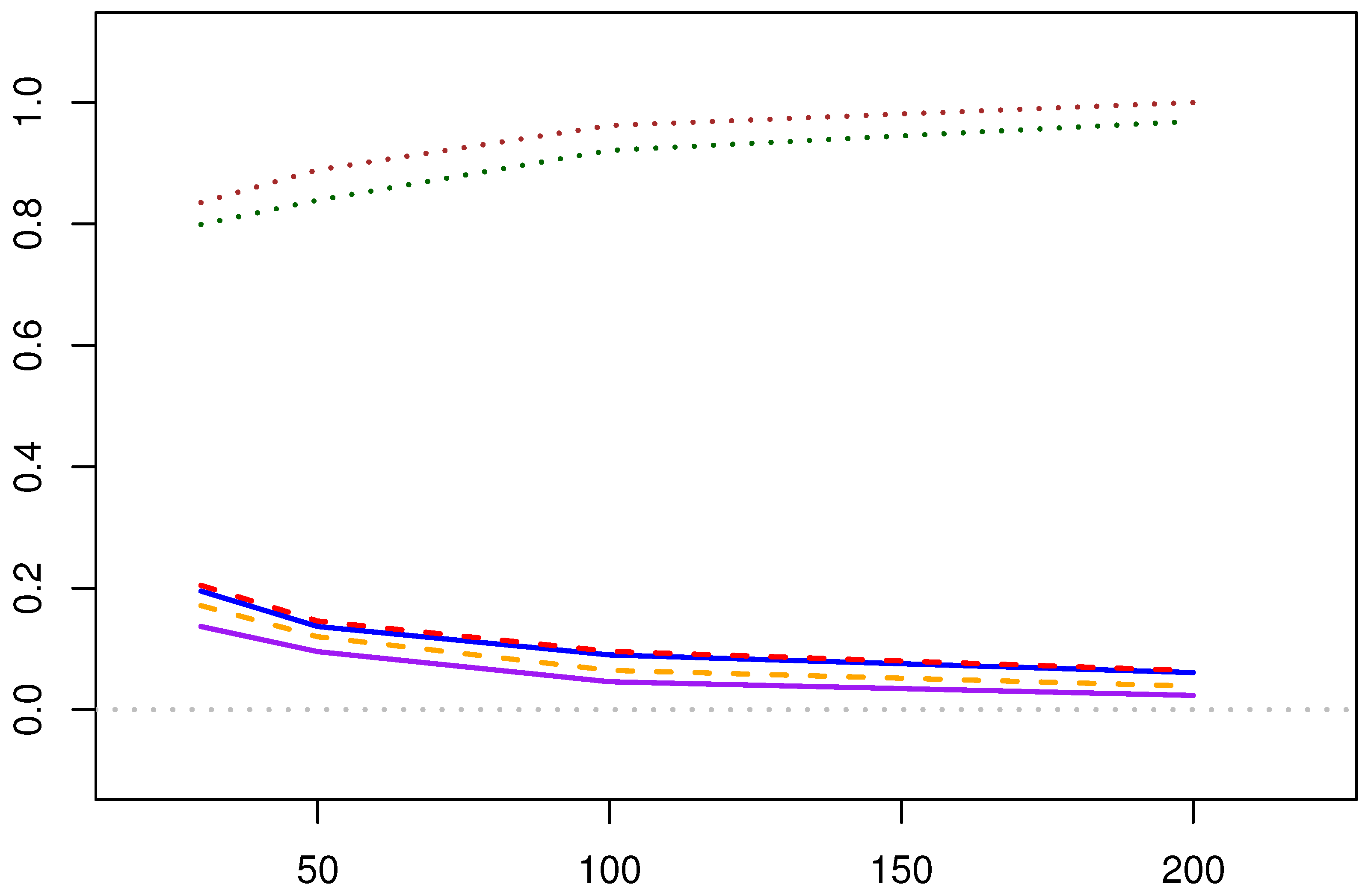
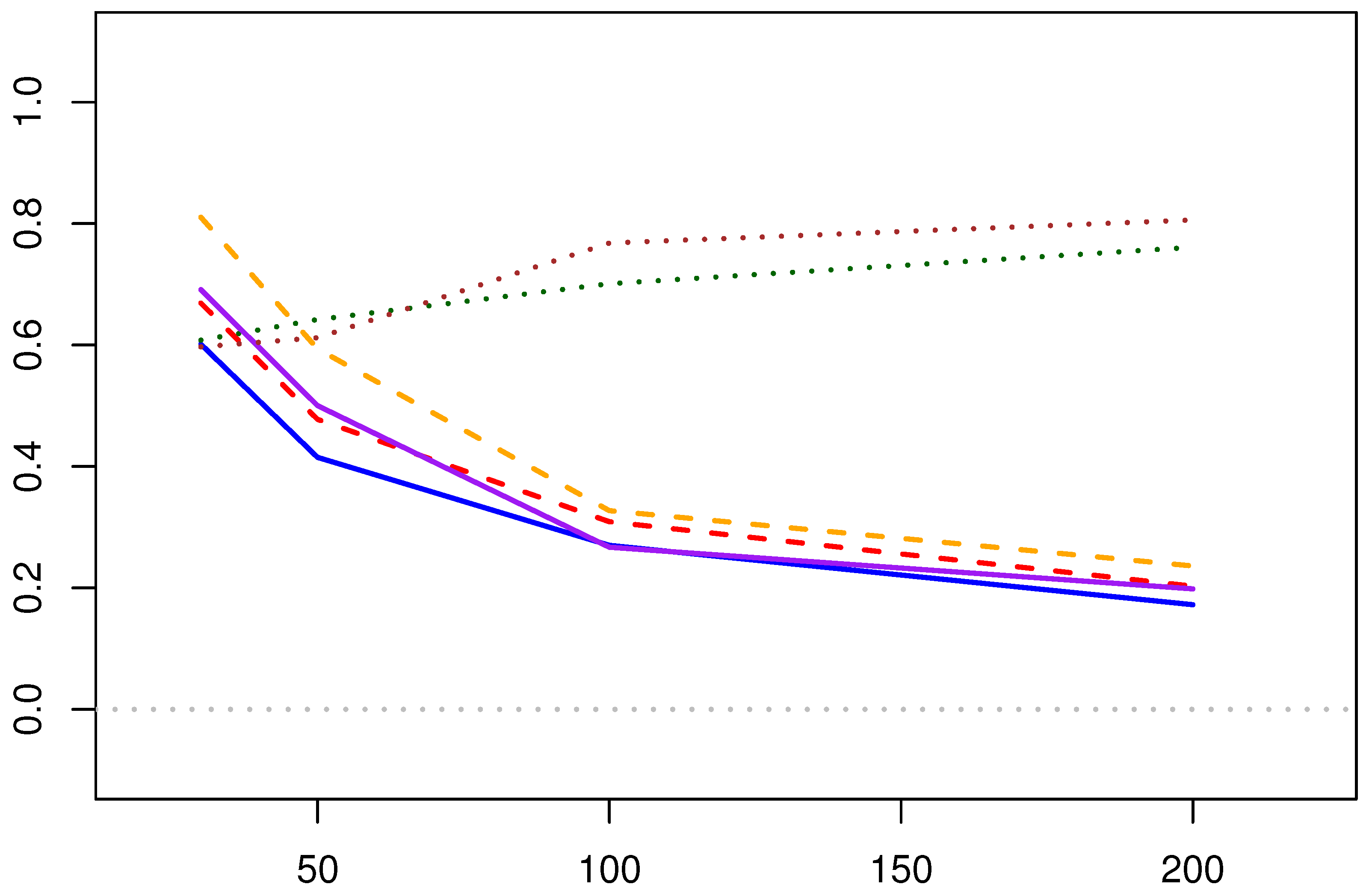
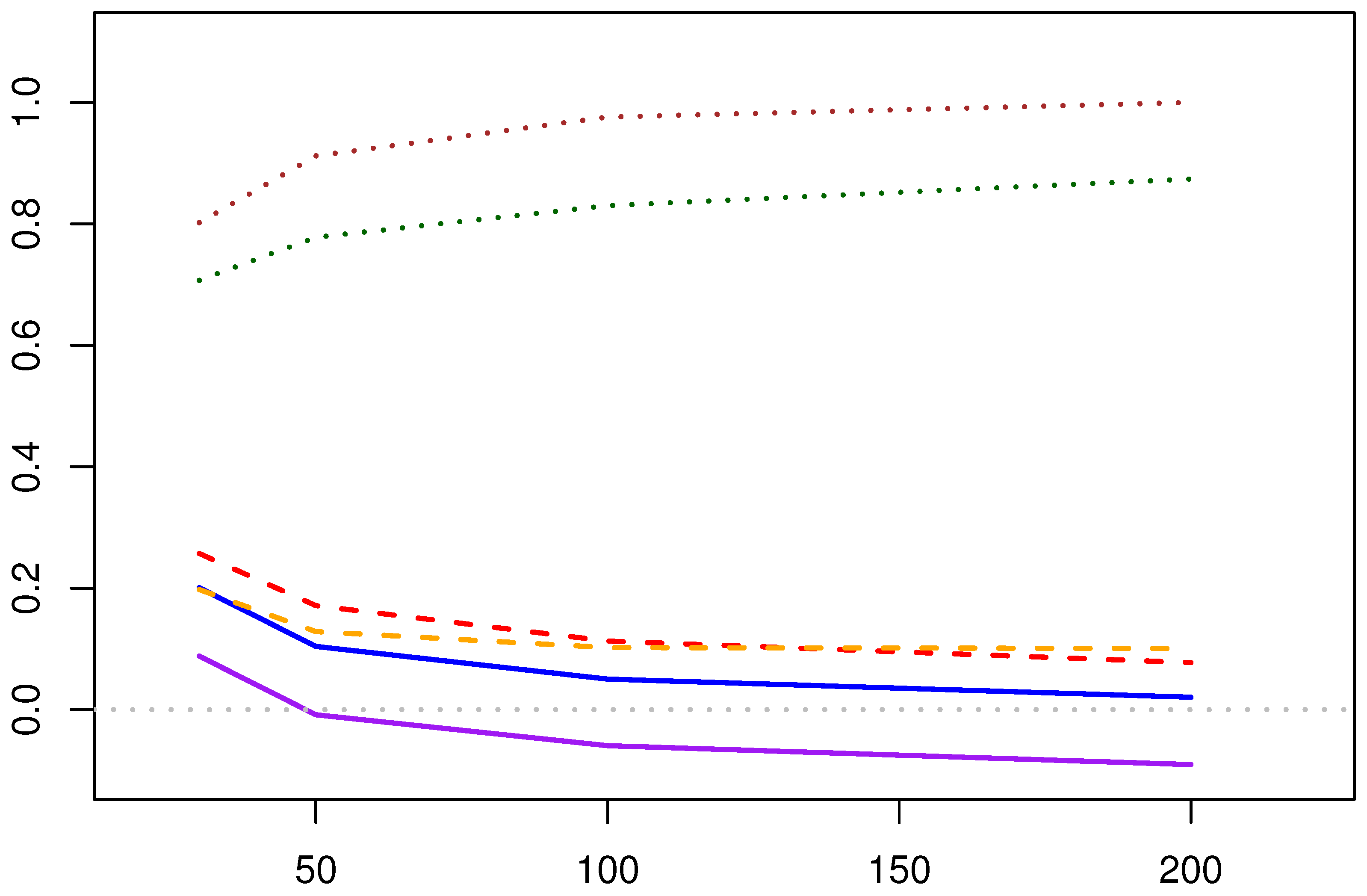
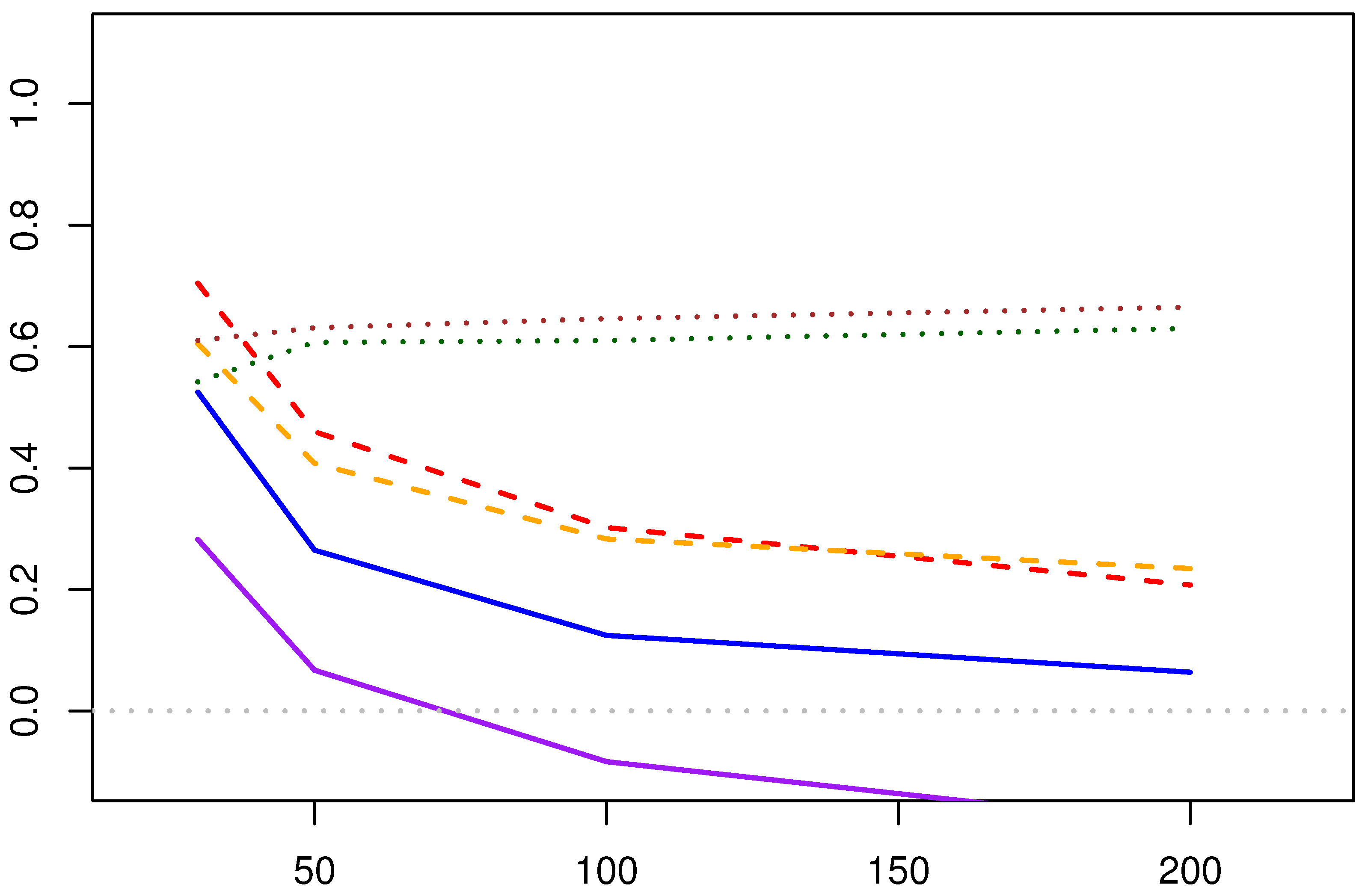
The figure below presents the line charts of the Newton–Raphson iteration method and the fixed-point estimation method in MPA estimation. With the legend given in Figure 4, Figure 5, Figure 6, Figure 7, Figure 8, Figure 9 and Figure 10 present line graphs drawn based on Table 1 and Table 2. Through these line charts, we can more intuitively make horizontal comparisons of the linear loss, mean absolute error, and confidence interval coverage rate of the parameter estimation results between the two methods, as well as vertical comparisons of the changes in estimation accuracy under different sample sizes. This intuitive comparison allows us to comprehensively evaluate the strengths and weaknesses of the two methods.
Considering that parameter estimation in real scenarios requires not only the accuracy of computational results but also computational efficiency, we introduce a new metric: computation time per cycle. The computation time per cycle is obtained by dividing the total calculation time by the total number of simulation cycles H. This metric is used to compare the computational efficiency of different methods, and the corresponding formula is Formula (44).
Computation time per cycle = Total cycle time H .
The computational efficiency of the two estimation methods under different parameter combinations and data scales is shown in Table 3. Here, FP represents the computation time per cycle of the fixed-point estimation method, and NR represents the computation time per cycle of the Newton–Raphson iteration method.
In this simulation data estimation, after generating the data, we performed censoring on it. The endpoints of the censoring intervals follow exponential distributions with parameters 0.5 and 1, respectively. Censoring was applied to each data point; if the data fell within the censoring interval, it was replaced by the interval; otherwise, no censoring occurred. The number of estimation repetitions, H, was set to 1000. The initial shape and scale parameters for the first iteration followed exponential distributions with parameters 0.5 and 1, respectively.
Comparing the results of the MPA parameter estimation using the fixed-point estimation method and the Newton–Raphson iteration method, we can draw the following conclusions:
  • Computational Efficiency: The Newton–Raphson iteration method optimizes the two parameters by iterating the negative log-likelihood function, yielding the estimation results. The fixed-point estimation method, by incorporating the relationship between the two parameters of the Lomax distribution, simplifies the optimization process. In terms of computational efficiency, the fixed-point method is relatively more efficient.
  • Point Estimation Results:
    (1)
    As the sample size increases, the linear and absolute errors of both estimation methods decrease correspondingly (applicable to both the shape and scale parameters). When the sample size reaches a certain level, the trend of error reduction slows down. Therefore, it can be seen that in practical applications, a moderate number of sample points can yield satisfactory estimation results. Sampling too many points increases the workload while providing limited improvement in the accuracy of the estimation results.
    (2)
    Compared with the results of the three sets of parameters, the Newton–Raphson iteration method of the MPA estimation methods overall outperforms the fixed-point solution, especially in the estimation of the shape parameter θ , where its advantage is more pronounced.
    (3)
    The estimation of scale parameter λ is not as good as that of shape parameter θ .
  • Interval Estimation Results:
    (1)
    The coverage rate of the confidence intervals for the two parameters in the Newton–Raphson iteration method increases with the increase of the initial sample size. The coverage rate of the confidence interval for the shape parameter is particularly satisfactory. However, for the fixed-point estimation method, there is a situation where the confidence interval coverage rate decreases as the amount of data increases, which is speculated to be due to the interval estimation itself not being suitable for application to the fixed-point estimation method.
    (2)
    The Newton–Raphson iteration method of the MPA estimation methods generally yields better coverage rates for the confidence intervals compared to the fixed-point estimation method.
In addition, we also notice that the proportion of outliers decreases when the data volume is large. This indicates that increasing the data volume can enhance the convergence of the estimation results in the simulation experiments and reduce the occurrence of outliers.
Considering the comparison results of the two MPA estimation methods mentioned above, the method with better overall performance, namely the Newton–Raphson solution, is selected for further comparison with the EM algorithm in the following text.

5.1.2. Comparison of the EM Algorithm and MPA Estimation

In this simulation data estimation, the same data generation and censoring schemes are employed, and the same outlier removal method is applied to the results, thus obtaining the relevant results in Table 4 and Table 5.
In the EM algorithm experiment above, we use the exponential distribution with the mean of 2 to generate the iterative initial values of the shape parameters, and the exponential distribution with the mean of 1 to generate the iterative initial values of the scale parameters.
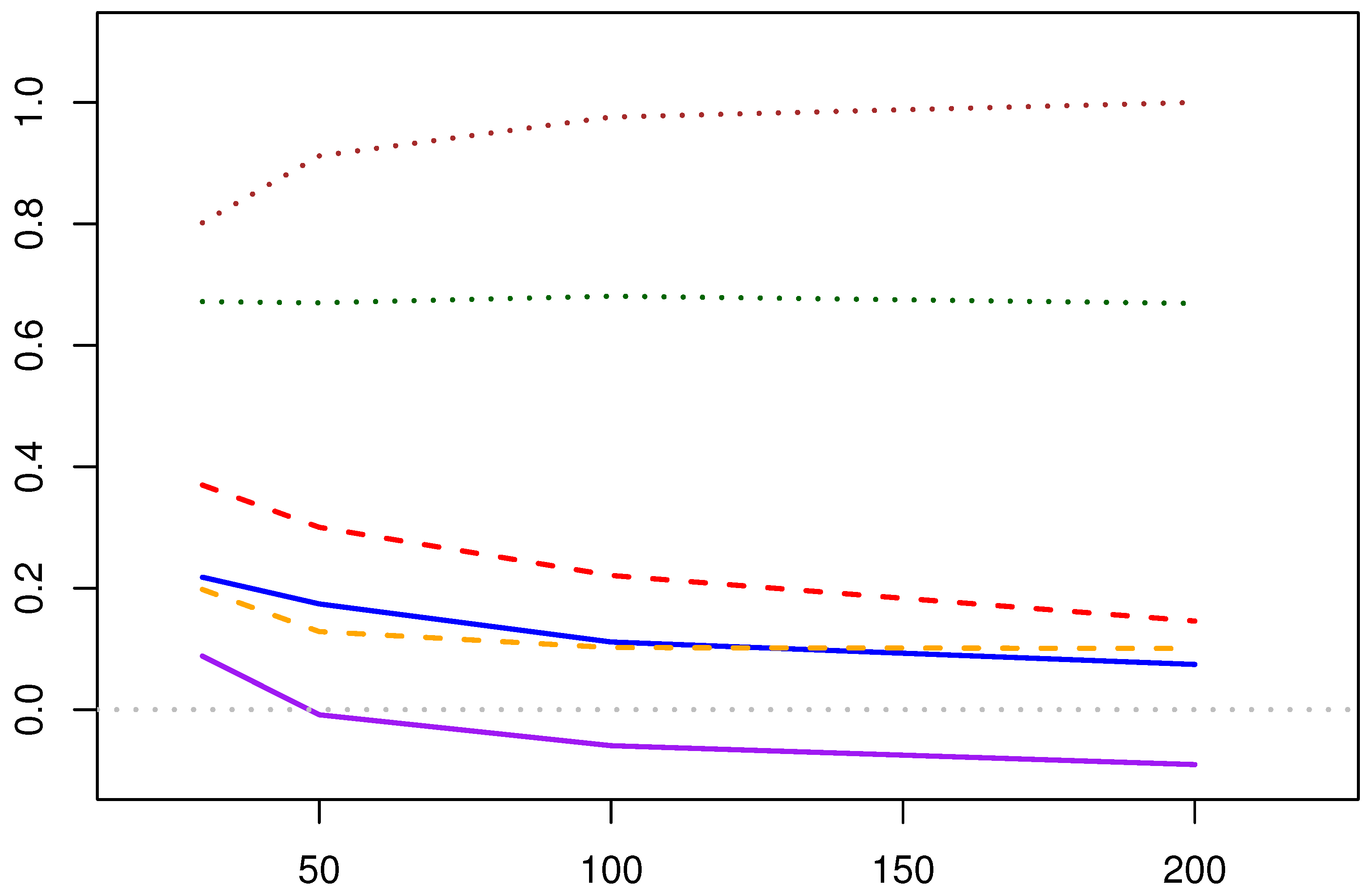
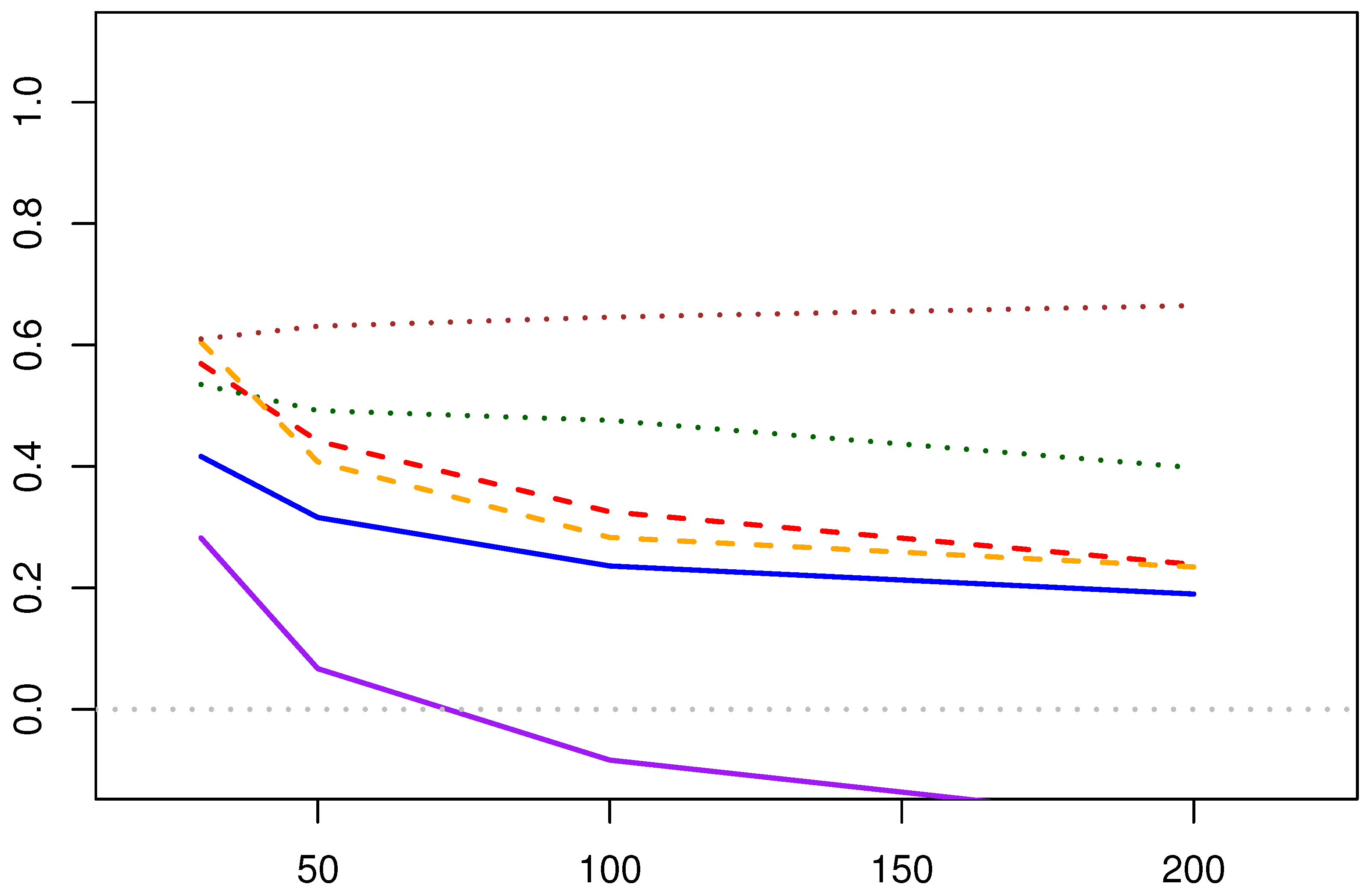
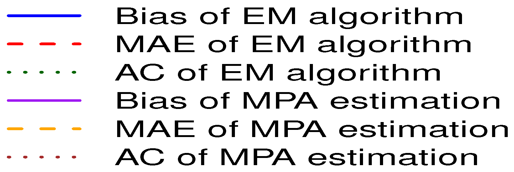
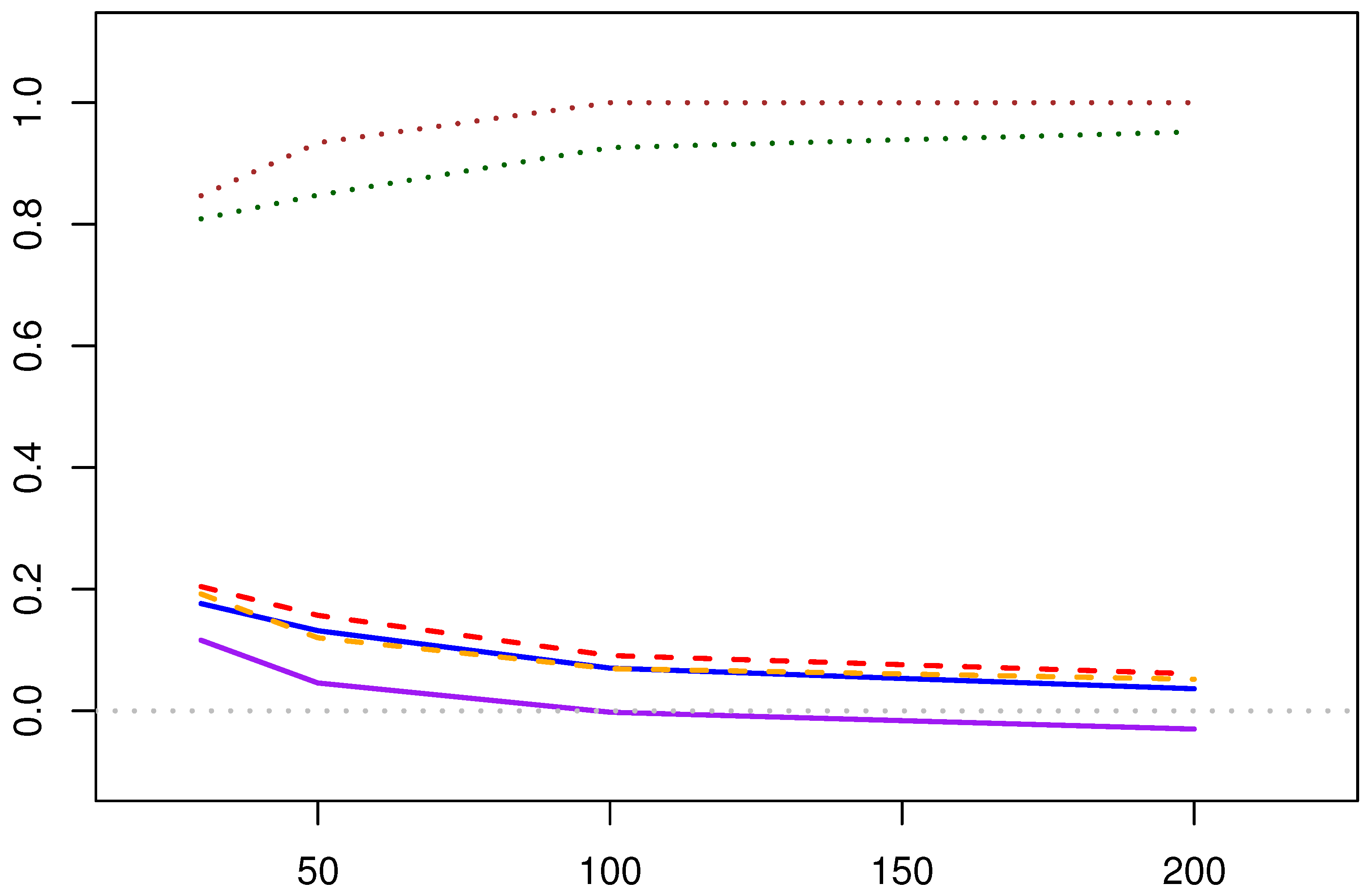
Similarly, for the convenience of intuitive comparison, with Figure 11 serves as the legend of Figure 12, Figure 13, Figure 14, Figure 15, Figure 16 and Figure 17, the relevant line charts are drawn as Figure 12, Figure 13, Figure 14, Figure 15, Figure 16 and Figure 17 present line graphs drawn based on tables.
From the tables, we can draw the following conclusions:
  • Computational Efficiency: As can be seen from Table 6, the Newton–Raphson solution for MPA estimation runs faster than the EM algorithm. This is because MPA does not require iteration over the samples, whereas the EM algorithm needs to perform sample iteration and integration operations.
  • Point Estimation Results:
    (1)
    Both the maximum likelihood estimates obtained by the EM algorithm and the MPA estimates obtained by the Newton–Raphson method show significant bias when the sample size is small, but achieve higher accuracy when the sample size is large.
    (2)
    In terms of estimating the shape parameter, the two estimation methods have similar estimation errors overall. However, when estimating the scale parameter, the EM algorithm provides more accurate results with smaller errors.
  • Interval Estimation Results:
    (1)
    In terms of confidence interval coverage, the confidence interval coverage of shape parameter θ by both algorithms is inferior to the confidence interval coverage of shape parameter θ estimates. It is speculated that the nature of the scale parameter causes this phenomenon.
    (2)
    As the amount of data increases, the confidence interval coverage of the estimated results of both methods increases.
Similarly, we can see from the results that the proportion of outliers decreases when the data volume is large.

5.1.3. Bayesian Estimation Results for the Shape Parameter

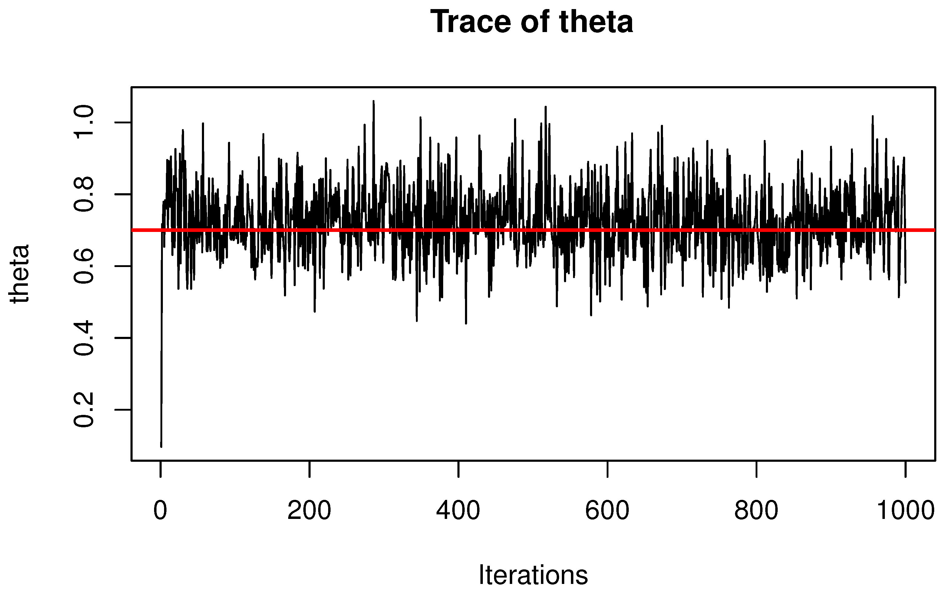
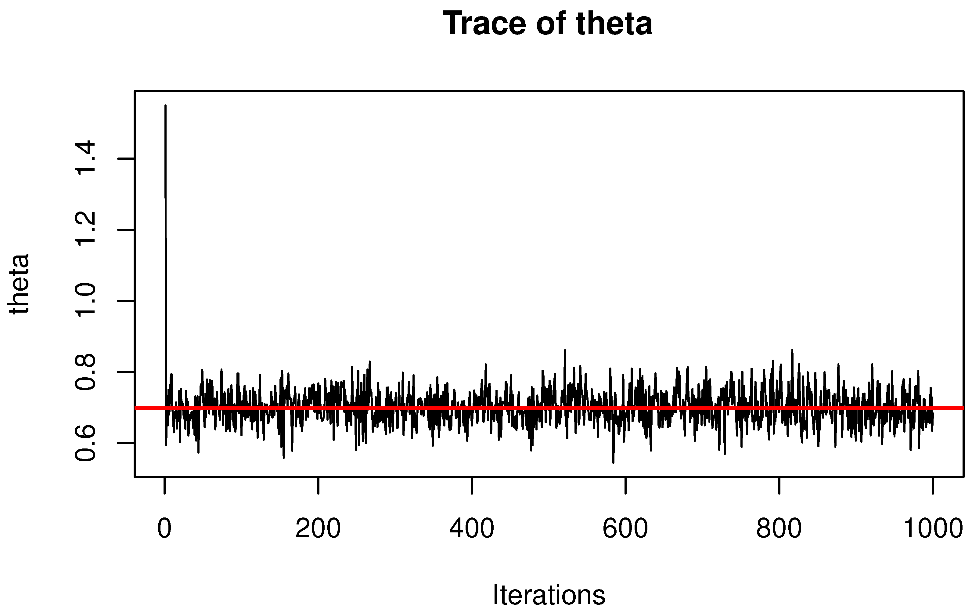
Before using Gibbs sampling for estimation, the convergence of the sampling results should first be verified. We selected the parameter combination ( θ , λ ) = ( 0.7 , 0.7 ) and plotted the trace plots of the sampling results when the sample sizes were 1000 and 1500, respectively.
From the Figure 18 and Figure 19, we can observe that the sampling results have become stable, with relatively fixed ranges of fluctuation. Most of the values (black line) fluctuate around the initially set parameter results, which are represented by the red line. Moreover, the range of fluctuation becomes narrower when the sample size is larger, indicating that the parameters have converged. After conducting tests with other parameter combinations, we obtained the same results. Therefore, we can demonstrate that the Bayesian estimation of the Lomax shape parameter under middle-censoring using Gibbs sampling is both scientific and reliable.
After numerically verifying the convergence of the Gibbs sampling estimates, we also experiment with the choice of hyperparameters for the prior distribution. The results show that the impact of different hyperparameter choices on the estimation error is very subtle. The inferred reason is that during the sampling process, the hyperparameters are iterated continuously, and the results gradually converge around the correct estimates. The values influenced by the initial hyperparameters have been discarded and thus do not significantly affect the results. In the subsequent simulation experiments, we estimated the Bayesian estimation accuracy and confidence interval coverage of the shape parameter θ under different numbers of Gibbs sampling iterations.
In the simulation experiments, the number of periods N is set to 1000. From the trace plots of the sampling samples, we can see that the samples converge quickly. Therefore, we set the number of initial samples to be discarded Q to 100 to ensure the accuracy of the estimation results and the efficiency of the computational process. To compare the impact of the number of samples on the estimation results, we conducted experiments with 200, 500, and 1000 samples, respectively. The hyperparameters in the prior distribution are chosen as a = 2.5 and b = 5 .
From Table 7, it can be concluded that the Bayesian estimation of the shape parameter, under the condition of a known scale parameter, achieves good fitting results. As the sample size increases, the accuracy significantly improves. When the number of initial samples discarded is 100, taking 500 sampling counts versus 1000 sampling counts does not significantly affect the accuracy of the results. Therefore, using an appropriate number of samples can yield good estimation results while saving computational power.

5.2. Real Data Analysis

When testing the estimation method for the following two sets of real data sets, we still used the same method of setting the initial iteration values in the simulation experiment and the same hyperparameter selection.

5.2.1. COVID-19 Datasets

According to the daily COVID-19 death counts divided by the number of new cases reported in [15], we obtain a set of real data samples that conform to the Lomax lifetime distribution.
Using the truncated interval of the exponential distribution with endpoints following parameters 10 and 30, we perform middle-censoring for each data point and obtain the data shown in Table 8.
Estimation results for complete data: θ = 8.9602 , λ = 1.1554 . The estimated results of the truncated data are shown in Table 9 and Table 10, which are in line with theoretical expectations.

5.2.2. Global Extreme Weather and Climate Disaster Event Loss Datasets

The Global Extreme Weather and Climate Disaster Loss Dataset for 2000–2021 [29] covers data related to extreme weather and climate disaster events worldwide during the period from 2000 to 2021. We selected the number of fatalities caused by these disasters from 2017 to 2021 as the subject of our analysis. After detailed data processing and statistical analysis, we found that the data essentially conform to the Lomax distribution.
Using the truncated interval of the exponential distribution with endpoints following parameters 0.002 and 0.001, we perform middle-censoring for each data point and obtain the data shown in Table 11.
Estimation results for complete data: θ = 2.9346 , λ = 653.5948 . The estimated results of the truncated data are shown in Table 12 and Table 13. In this practical application, the advantages of the EM algorithm are better demonstrated.

6. Summary and Future Prospects for Parameter Estimation of Lomax Distribution Under Middle-Censoring Data

In the field of Lomax parameter estimation with middle-censored data, this paper makes the following contributions:
  • In this paper, the details of EM algorithm for estimating two unknown parameters of Lomax distribution in middle-censored data are presented, and the results are verified by simulation experiments.
  • We propose two computational methods for parameter estimation after processing data using the Midpoint Approximation Method (MPA): the Newton–Raphson iteration method and the fixed-point method.
  • We calculate the ACIs for the two parameters in the middle-censored data, and take the covering probability of the confidence interval as one of the criteria to evaluate the estimation performance. The effectiveness of each estimation method is tested, and the applicability of the asymptotic confidence interval under intermediate censored data is also evaluated.
  • In the Bayesian estimation framework, we specifically estimate the shape parameter under middle-censoring using the Gamma prior distribution and the Gibbs sampling method, achieving satisfactory estimation results.
  • Through experiments with both simulated and real data, we validate the effectiveness and applicability of the proposed methods.
Based on the methods and achievements presented in this paper, the following future prospects are proposed, along with potential solutions and a ranking according to their importance:
(1)
This paper only experiments with data where the middle-censoring endpoints follow an exponential distribution, without discussing the impact of different distributions of the censoring interval endpoints on estimation, such as the Weibull distribution, uniform distribution, etc. Most of the current research on middle-censoring focuses on endpoints that follow an exponential distribution. Not only for the Lomax distribution, but also for other distributions, the study of different distributions of the endpoints of middle-censoring intervals holds research value.
(2)
In Bayesian estimation, we only discuss the estimation of the shape parameter θ when the scale parameter λ is known. However, in practice, it is rare to encounter situations where only one parameter needs to be estimated. Therefore, the Bayesian estimation of both parameters is an important issue that needs to be addressed in the future. Additionally, our Bayesian estimation only considers the Gamma distribution as the prior distribution, without discussing other types of prior distributions, such as non-informative priors or Jeffreys priors.
(3)
In simulation experiments, the estimation of confidence intervals is affected by the randomness of generating and censoring data, leading to situations where confidence intervals cannot be calculated. Therefore, the calculation of confidence interval coverage is based on the premise of generating middle-censored data for which progressive confidence intervals can be calculated. Another problem is that the asymptotic confidence interval coverage of scale parameters in simulation experiments is not high, which may be related to the nature of the parameters and the insufficient amount of data required for asymptotic confidence interval calculation. To address these interval estimation-related issues, Monte Carlo simulation can be considered to estimate confidence intervals in the future, or modified asymptotic confidence intervals can be adopted.
(4)
Regarding the existence and uniqueness of the maximum likelihood estimation solution for the parameters of the Lomax distribution under middle-censored data, this paper does not provide theoretical proof due to the complexity of the formulas. Future research needs to continue exploring the parameter estimation problems for related distributions under middle-censored data to further improve research in this area.
(5)
The EM algorithm has achieved good results in parameter estimation for the Lomax distribution under middle-censored data. However, during its operation, the issue of long computational time has arisen. In future research, the EM algorithm can be optimized through methods such as optimizing initial parameters, changing convergence criteria, and parallel computing. This will increase its computational speed while ensuring its accuracy.

Author Contributions

Conceptualization: P.R. and W.G.; Methodology: P.R. and W.G.; Software: P.R. and S.L.; Investigation: P.R. and S.L.; Writing—Original Draft: P.R.; Writing—Review and Editing: W.G.; Supervision: W.G. All authors have read and agreed to the published version of the manuscript.

Funding

This research was supported by Project 202510004172 which was supported by National Training Program of Innovation and Entrepreneurship for Undergraduates. Wenhao’s work was partially supported by the Science and Technology Research and Development Project of China State Railway Group Company, Ltd. (No. N2023Z020).

Data Availability Statement

The data presented in this study are openly available in [15,29].

Conflicts of Interest

The authors declare no conflicts of interest.

Appendix A

Theorem A1. 
The Gamma distribution is a conjugate prior distribution of the shape parameters of the Lomax life distribution.
Proof. 
Suppose the sample data is denoted as data, consisting of n sample data points, which are t 1 , t 2 , , t n , respectively.
The prior distribution of shape parameters is the Gamma distribution of parameters a and b, which is shown as follows:
π ( θ ) = b a Γ ( a ) θ a 1 e b θ .
Suppose the experimental data as data; then, the likelihood function of data can be represented as p ( data θ ) , and the joint distribution of data and θ is h ( data , θ ) . By integrating h ( data , θ ) over the parameter space Θ , we can obtain the marginal density of data, denoted as m ( data ) .
p ( d a t a | θ ) = θ n λ n i = 1 n 1 + t i λ θ + 1
h ( d a t a , θ ) = p ( d a t a | θ ) π ( θ ) = θ n λ n i = 1 n 1 + t i λ θ + 1 b a Γ ( a ) θ a 1 e b θ .
The posterior distribution of the shape parameters obtained by computational simplification is as follows:
π θ | d a t a θ n i = 1 n 1 + t i λ θ θ a 1 e b θ .
Thus, the conditional posterior distribution of the shape parameter is
G a m m a n + a , b + i = 1 n ln 1 + t i λ .
To sum up, we prove that the posterior distribution obtained when the Gamma distribution is selected as the prior distribution of the shape parameter is also the Gamma distribution. Therefore, the Gamma distribution is a conjugate prior distribution of the Lomax shape parameters.

References

  1. Leiderman, P.H.; Babu, B.; Kagia, J.; Kraemer, H.C.; Leiderman, G.F. African Infant Precocity and Some Social Influences during the First Year. Nature 1973, 242, 247–249. [Google Scholar] [CrossRef] [PubMed]
  2. Groeneboom, P.; Wellner, J.A. Information Bounds and Nonparametric Maximum Likelihood Estimation; Birkhäuser: Basel, Switzerland, 1992; Volume 19. [Google Scholar]
  3. Schick, A.; Yu, Q. Consistency of the GMLE with Mixed Case Interval-Censored Data. Scand. J. Stat. 2000, 27, 45–55. [Google Scholar] [CrossRef]
  4. Huang, J. Asymptotic properties of nonparametric estimation based on partly interval-censored data. Stat. Sin. 1999, 9, 501–520. [Google Scholar]
  5. Jammalamadaka, S.R.; Mangalam, V. Nonparametric estimation for middle-censored data. J. Nonparametr. Stat. 2003, 15, 253–265. [Google Scholar] [CrossRef]
  6. Jammalamadaka, S.R.; Iyer, S.K. Approximate self-consistency for middle-censored data. J. Stat. Plan. Inference 2004, 124, 75–86. [Google Scholar] [CrossRef]
  7. Yu, Q.Q.; Wong, G.Y.C.; Li, L.X. Asymptotic properties of self-consistent estimators with mixed interval-censored data. Ann. Inst. Stat. Math. 2001, 53, 469–486. [Google Scholar] [CrossRef]
  8. Iyer, S.K.; Jammalamadaka, S.R.; Kundu, D. Analysis of middle-censored data with exponential lifetime distributions. J. Stat. Plan. Inference 2008, 138, 3550–3560. [Google Scholar] [CrossRef]
  9. Bennett, N.A. Some Contributions to Middle-Censoring. Ph.D. Thesis, University of California, Santa Barbara, CA, USA, 2011; p. 3473719. Available online: https://www.proquest.com/dissertations-theses/some-contributions-middle-censoring/docview/896352567/se-2 (accessed on 1 June 2011).
  10. Yan, W.; Yimin, S.; Min, W. Statistical inference for dependence competing risks model under middle censoring. J. Syst. Eng. Electron. 2019, 30, 209–222. [Google Scholar] [CrossRef]
  11. Jammalamadaka, S.R.; Leong, E. Analysis of discrete lifetime data under middle-censoring and in the presence of covariates. J. Appl. Stat. 2015, 42, 905–913. [Google Scholar] [CrossRef]
  12. Lomax, K.S. Business failure: Another example of the analysis of the failure data. J. Am. Stat. Assoc. 1954, 49, 847–852. [Google Scholar] [CrossRef]
  13. Lun, Z.; Khattree, R. An overlooked Lomax-exponential connection. Commun. Stat.–Theory Methods 2022, 51, 26–28. [Google Scholar] [CrossRef]
  14. Aljohani, H.M. Estimation for the P(X > Y) of Lomax distribution under accelerated life tests. Heliyon 2024, 10, e25802. [Google Scholar] [CrossRef]
  15. Alsuhabi, H.; Alkhairy, I.; Almetwally, E.M.; Almongy, H.M.; Gemeay, A.M.; Hafez, E.H.; Aldallal, R.A.; Sabry, M. A superior extension for the Lomax distribution with application to COVID-19 infections real data. Alex. Eng. J. 2022, 61, 11077–11090. [Google Scholar] [CrossRef]
  16. Cramer, E.; Schmiedt, A.B. Progressively Type-II censored competing risks data from Lomax distributions. Comput. Stat. Data Anal. 2011, 55, 1285–1303. [Google Scholar] [CrossRef]
  17. Alfaer, N.M.; Aljohani, H.M. Balanced joint progressively hybrid Type-I censoring samples in estimating the lifetime Lomax distributions. Complexity 2021, 2021, 9929691. [Google Scholar] [CrossRef]
  18. El-Sherpieny, E.S.A.; Almetwally, E.M.; Muhammed, H.Z. Progressive Type-II hybrid censored schemes based on maximum product spacing with application to Power Lomax distribution. Phys. A Stat. Mech. Its Appl. 2020, 553, 124251. [Google Scholar] [CrossRef]
  19. Hasaballah, M.M.; Balogun, O.S.; Bakr, M.E. Non-Bayesian and Bayesian estimation for Lomax distribution under randomly censored with application. AIP Adv. 2024, 14, 025318. [Google Scholar] [CrossRef]
  20. Davarzani, N.; Parsian, A. Statistical inference for discrete middle-censored data. J. Stat. Plan. Inference 2011, 141, 1455–1462. [Google Scholar] [CrossRef]
  21. Giles, D.E.A.; Feng, H.; Godwin, R.T. On the Bias of the Maximum Likelihood Estimator for the Two-Parameter Lomax Distribution. Commun.-Stat.–Theory Methods 2013, 42, 1934–1950. [Google Scholar] [CrossRef]
  22. Dempster, A.P.; Laird, N.M.; Rubin, D.B. Maximum likelihood from incomplete data via the EM algorithm. J. R. Stat. Soc. Ser. B (Methodol.) 1977, 39, 1–22. [Google Scholar] [CrossRef]
  23. Wu, C.F.J. On the convergence properties of the EM algorithm. Ann. Stat. 1983, 11, 95–103. [Google Scholar] [CrossRef]
  24. Asl, M.N.; Belaghi, R.A.; Bevrani, H. Classical and Bayesian inferential approaches using Lomax model under progressively Type-I hybrid censoring. J. Comput. Appl. Math. 2018, 343, 397–412. [Google Scholar] [CrossRef]
  25. Turkson, A.; Ayiah-Mensah, F.; Nimoh, V. Handling censoring and censored data in survival analysis: A standalone systematic literature review. Int. J. Math. Math. Sci. 2021, 2021, 9307475. [Google Scholar] [CrossRef]
  26. Buzaridah, M.M.; Ramadan, D.A.; El-Desouky, B.S. Estimation of some lifetime parameters of flexible reduced logarithmic-inverse Lomax distribution under progressive Type-II censored data. J. Math. 2022, 2022, 1690458. [Google Scholar] [CrossRef]
  27. Okasha, H.; Lio, Y.; Albassam, M. On reliability estimation of Lomax distribution under adaptive Type-I progressive hybrid censoring scheme. Mathematics 2021, 9, 2903. [Google Scholar] [CrossRef]
  28. Kundu, D. Bayesian inference and life testing plan for the Weibull distribution in presence of progressive censoring. Technometrics 2008, 50, 144–154. [Google Scholar] [CrossRef]
  29. Yang, S.N. Global Extreme Weather and Climate Disaster Loss Dataset (2000–2021). 2023. Available online: https://data.casearth.cn/dataset/65388536819aec0f26f4c93a (accessed on 27 May 2023).
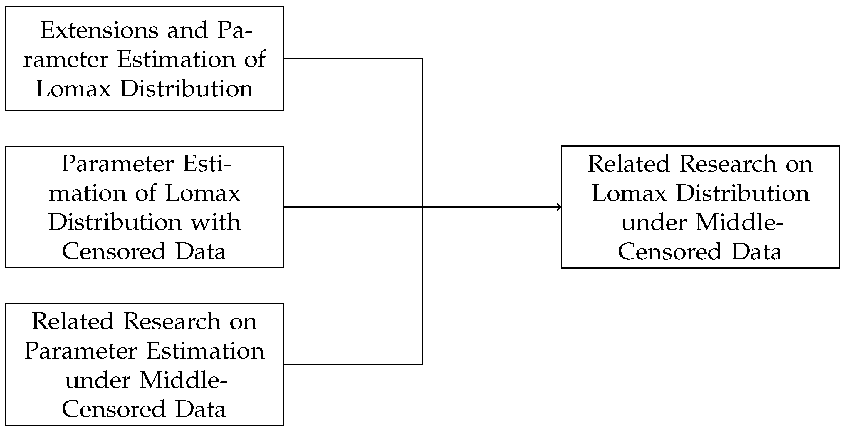
Figure 1. Research about the Lomax lifetime distribution and middle-censoring.
Axioms 14 00330 g001
Figure 2. Density curves of Lomax distribution with different parameters.
Axioms 14 00330 g002
Figure 3. Example of middle-censored data.
Axioms 14 00330 g003
Figure 4. The legend of the estimated result line chart in Figure 5, Figure 6, Figure 7, Figure 8, Figure 9 and Figure 10.
Axioms 14 00330 g004
Figure 5. Estimation results of the shape parameter θ under the parameter ( 0.7 , 0.7 ) . The legend is shown in Figure 4.
Axioms 14 00330 g005
Figure 6. Estimation results of the scale parameter λ under the parameter ( 0.7 , 0.7 ) . The legend is shown in Figure 4.
Axioms 14 00330 g006
Figure 7. Estimation results of the shape parameter θ under the parameter ( 0.6 , 0.9 ) . The legend is shown in Figure 4.
Axioms 14 00330 g007
Figure 8. Estimation results of the scale parameter λ under the parameter ( 0.6 , 0.9 ) . The legend is shown in Figure 4.
Axioms 14 00330 g008
Figure 9. Estimation results of the shape parameter θ under the parameter ( 0.8 , 1.1 ) . The legend is shown in Figure 4.
Axioms 14 00330 g009
Figure 10. Estimation results of the scale parameter λ under the parameter ( 0.8 , 1.1 ) . The legend is shown in Figure 4.
Axioms 14 00330 g010
Figure 11. The legend of the estimated result line chart in Figure 12, Figure 13, Figure 14, Figure 15, Figure 16 and Figure 17.
Axioms 14 00330 g011
Figure 12. Estimation results of the shape parameter θ under the parameter ( 0.7 , 0.7 ) . The legend is shown in Figure 11.
Axioms 14 00330 g012
Figure 13. Estimation results of the scale parameter λ under the parameter ( 0.7 , 0.7 ) . The legend is shown in Figure 11.
Axioms 14 00330 g013
Figure 14. Estimation results of the shape parameter θ under the parameter ( 0.6 , 0.9 ) . The legend is shown in Figure 11.
Axioms 14 00330 g014
Figure 15. Estimation results of the scale parameter λ under the parameter ( 0.6 , 0.9 ) . The legend is shown in Figure 11.
Axioms 14 00330 g015
Figure 16. Estimation results of the shape parameter θ under the parameter ( 0.8 , 1.1 ) . The legend is shown in Figure 11.
Axioms 14 00330 g016
Figure 17. Estimation results of the scale parameter λ under the parameter ( 0.8 , 1.1 ) . The legend is shown in Figure 11.
Axioms 14 00330 g017
Figure 18. Parameter ( θ , λ ) = ( 0.7 , 0.7 ) data size n = 50 .
Axioms 14 00330 g018
Figure 19. Parameter ( θ , λ ) = ( 0.7 , 0.7 ) data size n = 200 .
Axioms 14 00330 g019
Table 1. Comparison of shape parameter θ estimates between the fixed-point estimation and Newton–Raphson iteration methods.
( θ , λ ) nFixed-Point EstimationNewton–Raphson Iteration
BiasMAE AC θ ORBiasMAE AC θ OR
(0.7, 0.7)300.22690.25200.7220.0600.11610.19220.8470.048
500.14350.16170.8080.0570.04580.12010.9340.044
1000.09450.11110.8550.037−0.00220.06941.0000.037
2000.06400.07930.8830.021−0.03000.05201.0000.025
(0.6, 0.9)300.22490.29350.7260.0760.13690.17130.8350.090
500.15300.23040.7380.0460.09550.12000.8890.056
1000.08200.14810.7920.0390.04590.06470.9620.053
2000.05580.10760.8100.0200.02340.03881.0000.057
(0.8, 1.1)300.21810.36980.6720.0830.08820.19780.8020.072
500.17410.30030.6700.057−0.00850.12850.9120.061
1000.11140.22100.6810.037−0.05940.10220.9760.029
2000.07440.14590.6690.033−0.09050.10071.0000.016
Table 2. Comparison of scale parameter λ estimates between the fixed-point estimation and Newton–Raphson iteration methods.
( θ , λ ) nFixed-Point EstimationNewton–Raphson Iteration
BiasMAE AC λ ORBiasMAE AC λ OR
(0.7, 0.7)300.58950.63410.5390.0650.20030.41010.6090.080
500.39610.42850.5940.0500.11060.30020.6940.040
1000.26660.29260.6100.036−0.01520.17080.8260.033
2000.20370.21890.5770.026−0.06550.12520.8760.015
(0.6, 0.9)300.39970.46770.6130.0800.69120.81050.5970.086
500.27400.34120.6170.0630.50020.59370.6120.059
1000.19740.24980.5670.0270.26700.32720.7680.049
2000.13750.17040.5670.0280.19840.23610.8060.043
(0.8, 1.1)300.41650.56930.5350.0750.28230.60480.6100.076
500.31600.44180.4920.0590.06700.40760.6310.054
1000.23610.32530.4760.051−0.08360.28310.6460.030
2000.18990.23860.3980.037−0.18900.23450.6650.037
Table 3. Computation time per cycle of fixed-point estimation method and Newton–Raphson iteration method.
( θ , λ ) (0.7, 0.7)(0.6, 0.9)(0.8, 1.1)
n FPNRFPNRFPNR
300.001430.002590.002640.002660.002950.00235
500.001660.003740.001680.003650.002000.00267
1000.001900.005080.001830.005630.002480.00396
2000.002470.007480.002720.009350.002770.00713
Table 4. Comparison of shape parameter θ estimates between the EM Algorithm and Newton–Raphson iteration methods.
( θ , λ ) nEM AlgorithmNewton–Raphson Iteration
BiasMAE AC θ ORBiasMAE AC θ OR
(0.7, 0.7)300.17640.20430.8090.0710.11610.19220.8470.048
500.13180.15700.8480.0460.04580.12010.9340.044
1000.07030.09100.9260.032−0.00220.06941.0000.037
2000.03630.06090.9520.022−0.03000.05201.0000.025
(0.6, 0.9)300.19530.20470.7990.0740.13690.17130.8350.090
500.13690.14590.8390.0440.09550.12000.8890.056
1000.09010.09600.9210.0380.04590.06470.9620.053
2000.06100.06420.9690.0260.02340.03881.0000.057
(0.8, 1.1)300.20080.25720.7070.0740.08820.19780.8020.072
500.10410.17130.7780.058−0.00850.12850.9120.061
1000.05030.11290.8300.037−0.05940.10220.9760.029
2000.02040.07750.8740.025−0.09050.10071.0000.016
Table 5. Comparison of scale parameter λ estimates between the EM Algorithm and Newton–Raphson iteration methods.
( θ , λ ) nEM AlgorithmNewton–Raphson Iteration
BiasMAE AC λ ORBiasMAE AC λ OR
(0.7, 0.7)300.35430.43830.6620.0770.20030.41010.6090.080
500.25720.32740.6620.0490.11060.30020.6940.040
1000.12610.18520.7590.034−0.01520.17080.8260.033
2000.07940.13400.7850.013−0.06550.12520.8760.015
(0.6, 0.9)300.60130.66910.6080.0700.69120.81050.5970.086
500.41500.47760.6420.0570.50020.59370.6120.059
1000.27010.30900.7010.0290.26700.32720.7680.049
2000.17230.20280.7610.0270.19840.23610.8060.043
(0.8, 1.1)300.52490.70430.5420.0790.28230.60480.6100.076
500.26480.45980.6070.0600.06700.40760.6310.054
1000.12440.30200.6100.038−0.08360.28310.6460.030
2000.06370.20730.6300.020−0.18900.23450.6650.037
Table 6. Computation time per cycle of EM algorithm and MPA estimation method.
( θ , λ ) (0.7, 0.7)(0.6, 0.9)(0.8, 1.1)
n EMMPAEMMPAEMMPA
300.055420.002590.041470.002660.099930.00235
500.064080.003740.056070.003650.085040.00267
1000.121390.005080.109250.005630.153340.00396
2000.205630.007480.177320.009350.257660.00713
Table 7. Performance metrics for different settings.
( θ , λ ) nM = 200M = 500M = 1000
BiasMAE AC θ BiasMAE AC θ BiasMAE AC θ
(0.7, 0.7)300.04200.08600.9960.04010.09070.9980.03720.08550.994
500.02590.06991.0000.03440.07080.9980.02690.06970.998
1000.01550.05030.9990.01290.04890.9980.01050.04961.000
2000.00780.03641.0000.00720.03491.0000.00580.03551.000
(0.6, 0.9)300.07540.09180.9990.06590.09010.9990.06900.08880.996
500.05740.07190.9980.05580.07020.9990.05600.07240.996
1000.04460.05480.9990.03750.04950.9990.04170.05271.000
2000.02900.03621.0000.03030.03611.0000.02830.03561.000
(0.8, 1.1)30−0.00500.10290.993−0.00350.09540.9970.00090.09650.993
500.00850.08450.993−0.00820.08080.9980.00210.07700.998
100−0.00720.05850.996−0.00790.06030.998−0.00630.06060.996
200−0.00540.04410.999−0.00450.04180.998−0.00540.04270.998
Table 8. COVID-19 medical data after censoring treatment.
0.01490.00960.03220.05580.06360.06340.04670.0541
0.06100.02820.10210.08590.12660.17180.18960.1052
0.18860.10520.13940.16530.18650.15130.16070.1019
δ i = 0 0.14260.08351.08420.11170.11920.07260.07230.1573
n 1 = 70 0.06830.18420.15240.12420.10790.05900.12930.1068
0.07450.20470.19980.13400.35410.19600.19190.0975
0.24430.13110.02380.03930.03520.01570.30400.2362
0.07170.05580.11550.21630.11550.21630.09780.0888
0.09530.04910.21640.13100.13330.1124
(0.0190, 0.1672)(0.0035, 0.0657)(0.0193, 0.4777)(0.0403, 0.3831)
(0.0828, 0.6752)(0.0715, 0.8918)(0.0029, 0.3830)(0.1430, 0.5425)
(0.0803, 0.7193)(0.0105, 0.1338)(0.0315, 0.2710)(0.0057, 0.2977)
(0.0296, 0.1984)(0.0698, 0.2709)(0.0391, 0.6342)(0.0577, 0.2009)
δ i = 1 (0.0965, 0.3380)(0.0480, 0.0703)(0.0692, 0.2260)(0.0299, 0.1601)
n 2 = 37 (0.0206, 0.4020)(0.0573, 0.1095)(0.0243, 0.2168)(0.0061, 0.3026)
(0.0314, 0.1729)(0.0419, 0.2356)(0.1373, 0.4450)(0.0262, 0.2354)
(0.0949, 0.2687)(0.0567, 0.5827)(0.0516, 0.1286)(0.0099, 0.3902)
(0.0424, 0.2731)(0.0486, 0.4021)(0.0976, 0.2715)(0.0375, 0.3590)
(0.0385, 0.3161)
Table 9. Estimation results of double parameters for COVID-19 real data.
Estimation Results ( θ , λ ) Bias
EM(8.4261, 1.1237)(−0.5340, −0.0317)
MPA(9.5718, 1.2946)(0.6115, 0.1391)
Table 10. Estimation results of shape parameters for COVID-19 real data.
Estimation Results θ Bias
M = 2009.78460.8244
M = 5009.66750.7073
M = 10009.61980.6596
Table 11. Global extreme weather and climate disaster event loss data after censoring treatment.
78363059167184264284514
253251889714221211253
1825042468413617143119
1485359179300206725
δ i = 0 628128400188356190011599
n 1 = 75 5678683162257212146022
10719228228541019242556110
40011197211970116260
33521282201232268713
00457
(132.98, 1068.8)(290.67, 307.32)(137.82, 600.24)(838.38, 1264.8)
(80.467, 186.90)(120.93, 640.36)(2.3398, 1565.2)(155.36, 907.70)
δ i = 1 (58.948, 620.32)(62.411, 803.27)(295.84, 941.48)(244.63, 382.45)
n 2 = 25 (67.397, 191.28)(57.946, 1565.5)(163.48, 516.84)(75.673, 241.76)
(118.45, 165.72)(21.115, 298.93)(74.457, 212.94)(47.828, 588.44)
(696.11, 1202.0)(184.87, 603.93)(209.73, 255.58)(399.54, 752.28)
(37.435, 486.19)
Table 12. Estimation results of double parameters for global extreme weather and climate disaster event loss data.
Estimation Results ( θ , λ ) Bias
EM(2.9602, 688.3042)(0.0256, 34.7454)
MPA(2.0521, 394.2962)(−0.8825, −259.8826)
Table 13. Estimation results of shape parameters for global extreme weather and climate disaster event loss data.
Estimation Results θ Bias
M = 2002.8004−0.1342
M = 5002.8081−0.1265
M = 10002.7967−0.1379
Disclaimer/Publisher’s Note: The statements, opinions and data contained in all publications are solely those of the individual author(s) and contributor(s) and not of MDPI and/or the editor(s). MDPI and/or the editor(s) disclaim responsibility for any injury to people or property resulting from any ideas, methods, instructions or products referred to in the content.