Closed-Form Meromorphic Solutions of High-Order and High-Dimensional Differential Equations

Abstract

In this paper, we investigate closed-form meromorphic solutions of the fifth-order Sawada-Kotera (fSK) equation and (3+1)-dimensional generalized shallow water (gSW) equation. The study of high-order and high-dimensional differential equations is pivotal for modeling complex nonlinear phenomena in physics and engineering, where higher-order dispersion, dissipation, and multidimensional dynamics govern system behavior. Constructing explicit solutions is of great significance for the study of these equations. The elliptic, hyperbolic, rational, and exponential function solutions for these high-order and high-dimensional differential equations are achieved by proposing the extended complex method. The planar dynamics behavior of the (3+1)-dimensional gSW equation and its phase portraits are analyzed. Using computational simulation, the chaos behaviors of the high-dimensional differential equation under noise perturbations are examined. The dynamic structures of some obtained solutions are revealed via some 2D and 3D graphs. The results show that the extended complex method is an efficient and straightforward approach to solving diverse differential equations in mathematical physics.

1. Introduction

Nonlinear differential equations (NLDEs) play a crucial and widespread role in numerous domains of natural science and social science. These equations are extensively employed in various fields, including hydrodynamic systems, condensed matter physics, ionized gas studies, biological processes, photonic interactions, and chemical reactions. The investigation of closed-form solutions for different kinds of NLDEs has become a key aspect of contemporary mathematical research, with weighty implications for multiple scientific disciplines. These solutions provide essential tools for understanding complex phenomena in physical systems, advancing mathematical theory, and facilitating breakthroughs in various scientific fields. The development of solution methodologies for NLDEs not only enhances our theoretical framework but also enables practical applications in engineering, biological modeling, and materials science, establishing crucial connections between abstract mathematics and real-world problems. Numerous well-established systematic approaches for finding closed-form solutions of NLDEs have emerged, such as the Hirota bilinear method [1,2,3,4], Bernoulli $(G^{\prime }/G)$-expansion method [5], extended tanh expansion technique [6], sine-Gordon expansion approach [7,8], exp function method [9,10], modified Kudryashov method [11,12,13], exp$(-\phi (z\left)\right)$-expansion method [14,15,16,17], logistic method [18,19], and complex method [20,21,22,23].

A lot of approaches are constantly being improved and optimized. The Wiman–Valiron method [24] is a powerful analytical tool in the theory of entire and meromorphic functions. It investigates the asymptotic properties of transcendental entire functions within specific disks centered at points where their modulus reaches maximum values. This analytical framework has become instrumental in analyzing solutions to complex differential equations. Recently, Conte et al. [25] applied the Wiman–Valiron method to study a third-order nonlinear autonomous ordinary differential equation and obtained closed-form meromorphic solutions to the mentioned equation. A closed-form meromorphic solution to a given equation is a solution that can be explicitly expressed as the combination of elementary functions using a finite number of arithmetic operations and compositions. Additionally, the solution must be meromorphic in the complex plane, meaning it is holomorphic in the complex plane $\mathbb{C}$, except for the poles. Eremenko’s seminal work [26] established that all meromorphic solutions of the Kuramoto–Sivashinsky equation are expressible as elliptic functions or their degenerations. Subsequently, Kudryashov et al. [27,28] pioneered the application of Laurent series expansions to derive meromorphic exact solutions for specific classes of NLDEs. Building upon these advancements, Yuan et al. [29,30] formulated the complex method—an innovative synthesis of complex analytic theory and differential equation analysis—which effectively generates exact solutions for NLDEs, satisfying the $\langle p,q\rangle$ condition or being classified as Briot-Bouquet (BB) equations [31]. To overcome the limitations of the classical complex method, we developed the extended complex method, a novel framework capable of solving NLDEs that neither conform to the $\langle p,q\rangle$ condition nor belong to the BB family. This methodological extension broadens the scope of solvable equations. By performing a series of calculations and analysis, the extended complex method can uncover the underlying structure of the NLDE and lead to the construction of closed-form meromorphic solutions that accurately represent the corresponding physical or mathematical phenomena. The proposed technology shows great potential in solving nonlinear systems that were previously difficult to solve. We utilize this method to seek closed-form meromorphic solutions to the following two typical types of differential equations.

The fifth-order Sawada-Kotera equation [32] is given as follows:

$$u_{xxxxx}+15(u_x{u}_{xx}+u{u}_{xxx})+45u^2{u}_x+u_t=0.$$

(1)

It is a high-order NLDE that arises in the study of integrable systems and soliton theory. This fSK equation belongs to a class of completely integrable nonlinear evolution equations, which are notable for their rich mathematical structures, exact solvability, and connections to physical phenomena.

The (3+1)-dimensional generalized shallow water equation [33] is given in the following:

$$u_{xxxy}-3u_x{u}_{xy}-3u_{xx}{u}_y-u_{xz}+u_{yt}=0.$$

(2)

This high-dimensional equation represents a generalization of classical two-dimensional hydrodynamic models, incorporating an additional spatial dimension alongside temporal evolution. It is a significant model that describes various physical phenomena, such as fluid dynamics and wave propagation.

These two equations have attracted considerable attention from researchers to explore their solutions. Liu and Dai [34] employed the Hirota bilinear method on the fSK equation to derive 1-soliton solutions, singular periodic soliton solutions, and periodic 2-soliton solutions. Naher et al. [35] utilized the extended generalized Riccati equation mapping technique for constructing exact solutions for Equation (1). Guo et al. [36] applied the three-wave method to the fSK model, discovering periodic solitary and exact solitary solutions. Tang et al. [33] derived Grammian and Pfaffian solutions to the (3+1)-dimensional gSW equation with the assistance of Hirota bilinear method. Gu et al. [37] applied the Hirota bilinear method to Equation (2), yielding rational solutions and interaction solutions. Kumar and Kumar [38] investigated the gSW equation using the extended exponential rational function approach to obtain soliton solutions. Additionally, Shi et al. [39] developed multi-kink soliton solutions, resonant soliton molecules, and multi-lump solutions for Equation (2). Recently, Zhang et al. [40] proposed the generalized (3+1)-dimensional shallow water-like equation, and they found rational solutions and lump solutions by using the generalized bilinear method.

2. The Extended Complex Method

In this section, we will introduce the method used, and the specific steps are as follows:

Step 1. Transformation for PDE reduction.

Implement the transform $T:u(x,t)\to U\left(z\right)$, $(x,t)\to z$ into the PDE, yielding an ODE

$$F(U,U^{\prime },U^{″},\cdots )=0.$$

(3)

Step 2. Identification of the weak $\langle p,q\rangle$ criterion.

Presume the ODE admits a meromorphic solution U with at least one pole. If putting the Laurent series

$$U\left(z\right)=\sum _{k=-q}^{\infty }{G}_k{z}^k,q>0,G_{-q}\ne 0,$$

(4)

into Equation (3) yields p distinct Laurent principal parts

$$\sum _{k=-q}^{-1}{G}_k{z}^k,$$

where $q,p\in \mathbb{N}$, then we say that the weak $\langle p,q\rangle$ criterion for Equation (3) holds.

Step 3. Construction of meromorphic solutions with poles at the origin.

Before constructing the solutions, we need to introduce the special function. It is known that the Weierstrass elliptic function $\wp \left(z\right):=\wp (z,g_2,g_3)$ has double periods and satisfies

$${\left({\wp }^{\prime }\left(z\right)\right)}^2=4\wp {\left(z\right)}^3-g_2\wp \left(z\right)-g_3,$$

(5)

and it admits an addition formula [41] as follows:

$$\wp (z-z_0)=-\wp \left(z\right)+{\displaystyle \frac{1}{4}}{\left[{\displaystyle \frac{{\wp }^{\prime }\left(z\right)+{\wp }^{\prime }\left(z_0\right)}{\wp \left(z\right)-\wp \left(z_0\right)}}\right]}^2-\wp \left(z_0\right).$$

Inserting the indeterminate forms

$$\begin{array}{cc}\hfill U\left(z\right)=& {\displaystyle \sum _{i=1}^{h-1}\sum _{j=2}^q\frac{{(-1)}^j{\beta }_{-ij}}{(j-1)!}\frac{d^{j-2}}{d{z}^{j-2}}(\frac{1}{4}{\left[\frac{{\wp }^{\prime }\left(z\right)+D_i}{\wp \left(z\right)-C_i}\right]}^2-\wp \left(z\right))}\hfill \\ \hfill & {\displaystyle +\sum _{i=1}^{h-1}\frac{{\beta }_{-i1}}{2}\frac{{\wp }^{\prime }\left(z\right)+D_i}{\wp \left(z\right)-C_i}+\sum _{j=2}^q\frac{{(-1)}^j{\beta }_{-hj}}{(j-1)!}\frac{d^{j-2}}{d{z}^{j-2}}\wp \left(z\right)+{\beta }_0,}\hfill \end{array}$$

(6)

$$U\left(z\right)=\sum _{i=1}^h\sum _{j=1}^q{\displaystyle \frac{{\beta }_{ij}}{{(z-z_i)}^j}}+{\beta }_0,$$

(7)

$$U\left(e^{\alpha z}\right)=\sum _{i=1}^h\sum _{j=1}^q{\displaystyle \frac{{\beta }_{ij}}{{(e^{\alpha z}-e^{\alpha z_i})}^j}}+{\beta }_0,$$

(8)

into Equation (3), respectively, generates distinct systems of algebraic equations. The resolution of these systems produces three classes of close-form solutions with a pole at $z=0$, where $D_i^2=4C_i^3-g_2{C}_i-g_3$, and $R\left(z\right)$, $R\left(e^{\alpha z}\right)$$(\alpha \in \mathbb{C})$ contains $h(\le p)$ distinct poles of multiplicity q.

Step 4. Inverse transformational mapping to recover PDE solutions.

Applying the inverse transformation $T^{-1}$ to the meromorphic solutions U at an arbitrary pole yields exact solutions for the original PDE.

Remark 1.

Differential equations that satisfy the weak $\langle p,q\rangle$ criterion are applicable to the forms (6)–(8). It is an open problem regarding whether there are other meromorphic solutions that do not overlap with forms of (6)–(8).

3. Application of the Extended Complex Method to the fSK Equation

Insert

$$u(x,t)=U\left(z\right),z=\lambda x+\omega t,$$

into Equation (1) and integrate it to acquire

$$15{\lambda }^{3}U{U}^{″}+{\lambda }^5{U}^{\prime \prime \prime \prime }+\omega U+15\lambda U^3+\delta =0,$$

(9)

where $\delta$ is an integration constant.

Inserting (4) into Equation (9) yields $p=1,q=2$, so the weak $\langle 1,2\rangle$ criterion of Equation (9) holds.

Through the weak $\langle 1,2\rangle$ criterion and $h\le p$, we know that $h=1$ and $j=2$ in Equation (6), so the elliptic solutions of Equation (9) have the form of

$$U_{10}\left(z\right)={\beta }_{-12}\wp \left(z\right)+{\beta }_{20},$$

with a pole at $z=0$.

Putting $U_{10}\left(z\right)$ into Equation (9) yields

$$\sum _{i=1}^4{c}_{1i}{\wp }^{i-1}\left(z\right)=0,$$

(10)

where

$$c_{11}=-12{\lambda }^5{g}_3{\beta }_{-12}-{\displaystyle \frac{15{\lambda }^3{g}_2{\beta }_{-12}{\beta }_{20}}{2}}+15\lambda {\beta }_{20}^3+\omega {\beta }_{20}+\delta ,$$

$$c_{12}=-18{\lambda }^5{g}_2{\beta }_{-12}-{\displaystyle \frac{15{\lambda }^3{g}_2{\beta }_{-12}^2}{2}}+45\lambda {\beta }_{-12}{\beta }_{20}^2+\omega {\beta }_{-12},$$

$$c_{13}=90{\lambda }^3{\beta }_{-12}{\beta }_{20}+45\lambda {\beta }_{-12}^2{\beta }_{20},$$

$$c_{14}=120{\lambda }^5{\beta }_{-12}+90{\lambda }^3{\beta }_{-12}^2+15\lambda {\beta }_{-12}^3.$$

Equate all coefficients of some powers of $\wp \left(z\right)$ in Equation (10) with zero to yield the following algebraic equations:

$$c_{11}=0,c_{12}=0,c_{13}=0,c_{14}=0.$$

(11)

Solve Equation (11), and then

$${\beta }_{-12}=-2{\lambda }^2,{\beta }_{20}={\displaystyle \frac{\sqrt{5\lambda (3{\lambda }^5{g}_2-\omega )}}{15\lambda }},$$

$$\delta =-{\displaystyle \frac{1080{\lambda }^9{g}_3+2\sqrt{5\lambda \left(3{\lambda }^5{g}_2-\omega \right)}\lambda \left(24{\lambda }^5{g}_2+\omega \right)}{45{\lambda }^2}},$$

and

$${\beta }_{-12}=-2{\lambda }^2,{\beta }_{20}=-{\displaystyle \frac{\sqrt{5\lambda (3{\lambda }^5{g}_2-\omega )}}{15\lambda }},$$

$$\delta ={\displaystyle \frac{-2160{\lambda }^9{g}_3+\sqrt{5\lambda \left(3{\lambda }^5{g}_2-\omega \right)}\lambda \left(93{\lambda }^5{g}_2+2\omega \right)}{45{\lambda }^2}},$$

and then

$$U_{10}\left(z\right)=-2{\lambda }^2\wp \left(z\right)+{\displaystyle \frac{\sqrt{5\lambda (3{\lambda }^5{g}_2-\omega )}}{15\lambda }},$$

and

$$U_{20}\left(z\right)=-2{\lambda }^2\wp \left(z\right)-{\displaystyle \frac{\sqrt{5\lambda (3{\lambda }^5{g}_2-\omega )}}{15\lambda }}.$$

Therefore, the elliptic solutions of Equation (9) with an arbitrary pole are

$$U_1\left(z\right)=-2{\lambda }^2\wp (z-z_0)+{\displaystyle \frac{\sqrt{5\lambda (3{\lambda }^5{g}_2-\omega )}}{15\lambda }},$$

and

$$U_2\left(z\right)=-2{\lambda }^2\wp (z-z_0)-{\displaystyle \frac{\sqrt{5\lambda (3{\lambda }^5{g}_2-\omega )}}{15\lambda }},$$

where $z_0\in \mathbb{C}$.

Use the addition formula to $U_1\left(z\right)$ and $U_2\left(z\right)$, and then

$$U_1\left(z\right)=2{\lambda }^2\wp \left(z\right)-{\displaystyle \frac{{\lambda }^2}{2}}{\left({\displaystyle \frac{{\wp }^{\prime }\left(z\right)+D}{\wp \left(z\right)-C}}\right)}^2+{\displaystyle \frac{\sqrt{5\lambda (3{\lambda }^5{g}_2-\omega )}+30{\lambda }^{3}C}{15\lambda }},$$

and

$$U_2\left(z\right)=2{\lambda }^2\wp \left(z\right)-{\displaystyle \frac{{\lambda }^2}{2}}{\left({\displaystyle \frac{{\wp }^{\prime }\left(z\right)+D}{\wp \left(z\right)-C}}\right)}^2+{\displaystyle \frac{30{\lambda }^{3}C-\sqrt{5\lambda (3{\lambda }^5{g}_2-\omega )}}{15\lambda }},$$

where $C^2=4D^3-g_{2}D-g_3$, and $\delta =-{\displaystyle \frac{1080{\lambda }^9{g}_3+2\sqrt{5\lambda \left(3{\lambda }^5{g}_2-\omega \right)}\lambda \left(24{\lambda }^5{g}_2+\omega \right)}{45{\lambda }^2}}$ in the former case, and $\delta ={\displaystyle \frac{-2160{\lambda }^9{g}_3+\sqrt{5\lambda \left(3{\lambda }^5{g}_2-\omega \right)}\lambda \left(93{\lambda }^5{g}_2+2\omega \right)}{45{\lambda }^2}}$ in the latter case.

According to the weak $\langle 1,2\rangle$ criterion and $h\le p$, we know that i can only take 1, and j takes 1 and 2 in Equation (7). Set $z_1=0$; then, we have the indeterminate form of rational solutions

$$U_{30}\left(z\right)={\displaystyle \frac{{\beta }_{12}}{z^2}}+{\displaystyle \frac{{\beta }_{11}}{z}}+{\beta }_{10},$$

with a pole at $z=0$.

Substituting $U_{30}\left(z\right)$ into Equation (9) yields

$$\sum _{i=1}^7{c}_{2i}{z}^{i-7}=0,$$

(12)

where

$$c_{21}=120{\lambda }^5{\beta }_{12}+90{\lambda }^3{\beta }_{12}^2+15\lambda {\beta }_{12}^3,$$

$$c_{22}=24{\lambda }^5{\beta }_{11}+120{\lambda }^3{\beta }_{11}{\beta }_{12}+45\lambda {\beta }_{11}{\beta }_{12}^2,$$

$$c_{23}=90{\lambda }^3{\beta }_{10}{\beta }_{12}+30{\lambda }^3{\beta }_{11}^2+45\lambda {\beta }_{10}{{\beta }_{12}}^2+45\lambda {{\beta }_{11}}^2{\beta }_{12},$$

$$c_{24}=30{\lambda }^3{\beta }_{10}{\beta }_{11}+90\lambda {\beta }_{10}{\beta }_{11}{\beta }_{12}+15\lambda {\beta }_{11}^3,$$

$$c_{25}=45\lambda {\beta }_{10}^2{\beta }_{12}+45\lambda {\beta }_{10}{\beta }_{11}^2+\omega {\beta }_{12},$$

$$c_{26}=45\lambda {\beta }_{10}^2{\beta }_{11}+\omega {\beta }_{11},$$

$$c_{27}=15\lambda {\beta }_{10}^3+\omega {\beta }_{10}+\delta .$$

Set all coefficients of the same powers of z in Equation (12) to zero to attain the algebraic equations as the following:

$$c_{21}=0,c_{22}=0,c_{23}=0,c_{24}=0,c_{25}=0,c_{26}=0,c_{27}=0.$$

By solving the above equations, we obtain

$${\beta }_{12}=-2{\lambda }^2,{\beta }_{11}=0,{\beta }_{10}={\displaystyle \frac{\sqrt{-5\lambda \omega }}{15\lambda }},\delta =-{\displaystyle \frac{2\omega \sqrt{-5\lambda \omega }}{45\lambda }},$$

and

$${\beta }_{12}=-2{\lambda }^2,{\beta }_{11}=0,{\beta }_{10}=-{\displaystyle \frac{\sqrt{-5\lambda \omega }}{15\lambda }},\delta ={\displaystyle \frac{2\omega \sqrt{-5\lambda \omega }}{45\lambda }},$$

and then

$$U_{30}\left(z\right)=-{\displaystyle \frac{2{\lambda }^2}{z^2}}+{\displaystyle \frac{\sqrt{-5\lambda \omega }}{15\lambda }},$$

and

$$U_{40}\left(z\right)=-{\displaystyle \frac{2{\lambda }^2}{z^2}}-{\displaystyle \frac{\sqrt{-5\lambda \omega }}{15\lambda }},$$

where $\delta =-{\displaystyle \frac{2\omega \sqrt{-5\lambda \omega }}{45\lambda }}$ in the former case, and $\delta ={\displaystyle \frac{2\omega \sqrt{-5\lambda \omega }}{45\lambda }}$ in the latter case.

Insert $U\left(z\right)=R\left(\eta \right)$ into Equation (9), then

$$\begin{array}{c}{\lambda }^5{\alpha }^4(R^{\left(4\right)}{\eta }^4+6R^{\prime \prime \prime }{\eta }^3+7R^{\prime \prime }{\eta }^2+R^{\prime }\eta )+15{\lambda }^3{\alpha }^{2}R(\eta R^{\prime }+{\eta }^2{R}^{\prime \prime })\\ +15\lambda R^3+\omega R+\delta =0,\end{array}$$

(13)

where $\eta =e^{\alpha z}$ ($\alpha \in \mathbb{C}$).

By substituting

$$U_{50}\left(z\right)={\displaystyle \frac{b_{12}}{{(e^{\alpha z}-1)}^2}}+{\displaystyle \frac{b_{11}}{e^{\alpha z}-1}}+b_{10},$$

into Equation (13), we obtain that

$$\sum _{i=1}^7{c}_{3i}{\alpha }^2{e}^{(7-i)\alpha z}{(e^{\alpha z}-1)}^{-6}=0,$$

(14)

where

$$c_{31}=15\lambda b_{10}^3+\omega b_{10}+\delta ,$$

$$c_{32}={\alpha }^4{\lambda }^5{b}_{11}+15{\alpha }^2{\lambda }^3{b}_{10}{b}_{11}-90\lambda b_{10}^3+45\lambda b_{11}{b}_{10}^2-6\omega b_{10}+\omega b_{11}-6\delta ,$$

$$c_{33}=10{\alpha }^4{\lambda }^5{b}_{11}+16{\alpha }^4{\lambda }^5{b}_{12}-30{\alpha }^2{\lambda }^3{b}_{10}{b}_{11}+60{\alpha }^2{\lambda }^3{b}_{10}{b}_{12}+225\lambda b_{10}^3-5\omega b_{11}$$

$$+15{\alpha }^2{\lambda }^3{b}_{11}^2-225\lambda b_{11}{b_{10}}^2+45\lambda b_{12}{b_{10}}^2+45\lambda {b_{11}}^2{b}_{10}+15\omega b_{10}+\omega b_{12}+15\delta ,$$

$$c_{34}=66{\alpha }^4{\lambda }^5{b}_{12}-90{\alpha }^2{\lambda }^3{b}_{10}{b}_{12}-15{\alpha }^2{\lambda }^3{b}_{11}^2+75{\alpha }^2{\lambda }^3{b}_{11}{b}_{12}+450\lambda b_{11}{b}_{10}^2$$

$$-180\lambda b_{12}{b}_{10}^2-180\lambda {b_{11}}^2{b}_{10}+90\lambda b_{12}{b}_{11}{b}_{10}+15\lambda b_{11}^3-20\omega b_{10}+10\omega b_{11}-20\delta$$

$$-300\lambda b_{10}^3-4\omega b_{12},$$

$$c_{35}=-10{\alpha }^4{\lambda }^5{b}_{11}+36{\alpha }^4{\lambda }^5{b}_{12}+30{\alpha }^2{\lambda }^3{b}_{10}{b}_{11}-15{\alpha }^2{\lambda }^3{b}_{11}^2-30{\alpha }^2{\lambda }^3{b}_{11}{b}_{12}$$

$$+225\lambda b_{10}^3-450\lambda b_{11}{b}_{10}^2+270\lambda b_{12}{b}_{10}^2+270\lambda b_{11}^2{b}_{10}+45\lambda b_{10}{b}_{12}^2-45\lambda b_{11}^3$$

$$-270\lambda b_{12}{b}_{11}{b}_{10}+60{\alpha }^2{\lambda }^3{b}_{12}^2+45\lambda b_{11}^2{b}_{12}+15\omega b_{10}-10\omega b_{11}+6\omega b_{12}+15\delta ,$$

$$c_{36}=-{\alpha }^4{\lambda }^5{b}_{11}+2{\alpha }^4{\lambda }^5{b}_{12}-15{\alpha }^2{\lambda }^3{b}_{10}{b}_{11}+30{\alpha }^2{\lambda }^3{b}_{10}{b}_{12}-45{\alpha }^2{\lambda }^3{b}_{11}{b}_{12}$$

$$-180\lambda b_{11}^2{b}_{10}+30{\alpha }^2{\lambda }^3{b}_{12}^2-90\lambda b_{10}^3+225\lambda b_{11}{b}_{10}^2-180\lambda b_{12}{b}_{10}^2+15{\alpha }^2{\lambda }^3{b}_{11}^2$$

$$+270\lambda b_{12}{b}_{11}{b}_{10}-90\lambda b_{10}{b}_{12}^2+45\lambda b_{11}^3-90\lambda b_{11}^2{b}_{12}+45\lambda b_{11}{b}_{12}^2-6\omega b_{10}$$

$$+5\omega b_{11}-4\omega b_{12}-6\delta ,$$

$$c_{37}=15\lambda b_{10}^3-45\lambda b_{11}{b}_{10}^2+45\lambda b_{12}{b}_{10}^2+45\lambda b_{11}^2{b}_{10}-90\lambda b_{12}{b}_{11}{b}_{10}-15\lambda b_{11}^3$$

$$+45\lambda b_{10}{b}_{12}^2+45\lambda b_{11}^2{b}_{12}-45\lambda b_{11}{b}_{12}^2+15\lambda b_{12}^3+\omega b_{10}-\omega b_{11}+\omega b_{12}+\delta .$$

Let the coefficients of all powers about $e^{\alpha z}$ in Equation (14) be zero to obtain the algebraic equations as below:

$$c_{31}=0,c_{32}=0,c_{33}=0,c_{34}=0,c_{35}=0,c_{36}=0,c_{37}=0.$$

By solving the above equations, we obtain

$$b_{12}=-2{\lambda }^2{\alpha }^2,b_{11}=-2{\lambda }^2{\alpha }^2,b_{10}=-{\displaystyle \frac{{\lambda }^2{\alpha }^2}{6}},\omega ={\displaystyle \frac{{\lambda }^5{\alpha }^4}{4}},\delta ={\displaystyle \frac{{\lambda }^7{\alpha }^6}{9}}.$$

Thus, simply periodic solutions to Equation (9) with a pole at $z=0$ are

$$U_{50}\left(z\right)=-{\displaystyle \frac{2{\lambda }^2{\alpha }^2}{{(e^{\alpha z}-1)}^2}}-{\displaystyle \frac{2{\lambda }^2{\alpha }^2}{(e^{\alpha z}-1)}}-{\displaystyle \frac{{\lambda }^2{\alpha }^2}{6}}$$

$$=-{\displaystyle \frac{2{\lambda }^2{\alpha }^2{e}^{\alpha z}}{{(e^{\alpha z}-1)}^2}}-{\displaystyle \frac{{\lambda }^2{\alpha }^2}{6}}$$

$$=-{\displaystyle \frac{{\lambda }^2{\alpha }^2}{2}}{coth}^2{\displaystyle \frac{\alpha z}{2}}+{\displaystyle \frac{{\lambda }^2{\alpha }^2}{3}}.$$

Similar to $U_{50}\left(z\right)$, we substitute

$$U_{60}\left(z\right)={\displaystyle \frac{b_{12}}{{(e^{\alpha z}+1)}^2}}+{\displaystyle \frac{b_{11}}{e^{\alpha z}+1}}+b_{10},$$

into Equation (13) to yield

$$b_{12}=-2{\lambda }^2{\alpha }^2,b_{11}=2{\lambda }^2{\alpha }^2,b_{10}=-{\displaystyle \frac{{\lambda }^2{\alpha }^2}{6}},\omega ={\displaystyle \frac{{\lambda }^5{\alpha }^4}{4}},\delta ={\displaystyle \frac{{\lambda }^7{\alpha }^6}{9}},$$

then

$$U_{60}\left(z\right)=-{\displaystyle \frac{2{\lambda }^2{\alpha }^2}{{(e^{\alpha z}+1)}^2}}+{\displaystyle \frac{2{\lambda }^2{\alpha }^2}{(e^{\alpha z}+1)}}-{\displaystyle \frac{{\lambda }^2{\alpha }^2}{6}}$$

$$={\displaystyle \frac{2{\lambda }^2{\alpha }^2{e}^{\alpha z}}{{(e^{\alpha z}+1)}^2}}-{\displaystyle \frac{{\lambda }^2{\alpha }^2}{6}}$$

$$=-{\displaystyle \frac{{\lambda }^2{\alpha }^2}{2}}{tanh}^2{\displaystyle \frac{\alpha z}{2}}+{\displaystyle \frac{{\lambda }^2{\alpha }^2}{3}}.$$

Substituting

$$U_{70}\left(z\right)={\displaystyle \frac{b_{14}}{{(e^{\alpha z}-1)}^2}}+{\displaystyle \frac{b_{13}}{{(e^{\alpha z}+1)}^2}}+{\displaystyle \frac{b_{12}}{e^{\alpha z}-1}}+{\displaystyle \frac{b_{11}}{e^{\alpha z}+1}}+b_{10},$$

into Equation (13) yields

$$b_{14}=-2{\lambda }^2{\alpha }^2,b_{13}=-2{\lambda }^2{\alpha }^2,b_{12}=-2{\lambda }^2{\alpha }^2,b_{11}=2{\lambda }^2{\alpha }^2,$$

$$b_{10}=-{\displaystyle \frac{{\lambda }^2{\alpha }^2}{3}},\omega ={\displaystyle \frac{{\lambda }^5{\alpha }^4}{4}},\delta ={\displaystyle \frac{2{\lambda }^7{\alpha }^6}{9}},$$

and then

$$U_{70}\left(z\right)=-{\displaystyle \frac{2{\lambda }^2{\alpha }^2}{{(e^{\alpha z}-1)}^2}}-{\displaystyle \frac{2{\lambda }^2{\alpha }^2}{{(e^{\alpha z}+1)}^2}}-{\displaystyle \frac{2{\lambda }^2{\alpha }^2}{(e^{\alpha z}-1)}}+{\displaystyle \frac{2{\lambda }^2{\alpha }^2}{(e^{\alpha z}+1)}}-{\displaystyle \frac{{\lambda }^2{\alpha }^2}{3}}$$

$$=-{\displaystyle \frac{2{\lambda }^2{\alpha }^2{e}^{\alpha z}}{{(e^{\alpha z}-1)}^2}}+{\displaystyle \frac{2{\lambda }^2{\alpha }^2{e}^{\alpha z}}{{(e^{\alpha z}+1)}^2}}+{\displaystyle \frac{2{\lambda }^2{\alpha }^2}{3}}.$$

By collecting closed-form meromorphic solutions of Equation (9) in the above procedures, we obtain the following theorem.

Theorem 1.

The closed-form meromorphic solutions of the fSK equation with an arbitrary pole are

$$U_1\left(z\right)=2{\lambda }^2\wp \left(z\right)-{\displaystyle \frac{{\lambda }^2}{2}}{\left({\displaystyle \frac{{\wp }^{\prime }\left(z\right)+D}{\wp \left(z\right)-C}}\right)}^2+{\displaystyle \frac{\sqrt{5\lambda (3{\lambda }^5{g}_2-\omega )}+30{\lambda }^{3}C}{15\lambda }},$$

$$U_2\left(z\right)=2{\lambda }^2\wp \left(z\right)-{\displaystyle \frac{{\lambda }^2}{2}}{\left({\displaystyle \frac{{\wp }^{\prime }\left(z\right)+D}{\wp \left(z\right)-C}}\right)}^2+{\displaystyle \frac{30{\lambda }^{3}C-\sqrt{5\lambda (3{\lambda }^5{g}_2-\omega )}}{15\lambda }},$$

where $C^2=4D^3-g_{2}D-g_3$, with $\delta =-{\displaystyle \frac{1080{\lambda }^9{g}_3+2\sqrt{5\lambda \left(3{\lambda }^5{g}_2-\omega \right)}\lambda \left(24{\lambda }^5{g}_2+\omega \right)}{45{\lambda }^2}}$ in the former case, and $\delta ={\displaystyle \frac{-2160{\lambda }^9{g}_3+\sqrt{5\lambda \left(3{\lambda }^5{g}_2-\omega \right)}\lambda \left(93{\lambda }^5{g}_2+2\omega \right)}{45{\lambda }^2}}$ in the latter case;

$$U_3\left(z\right)=-{\displaystyle \frac{2{\lambda }^2}{{(z-z_0)}^2}}+{\displaystyle \frac{\sqrt{-5\lambda \omega }}{15\lambda }},$$

$$U_4\left(z\right)=-{\displaystyle \frac{2{\lambda }^2}{{(z-z_0)}^2}}-{\displaystyle \frac{\sqrt{-5\lambda \omega }}{15\lambda }},$$

where $\delta =-{\displaystyle \frac{2\omega \sqrt{-5\lambda \omega }}{45\lambda }}$ in the former case, and $\delta ={\displaystyle \frac{2\omega \sqrt{-5\lambda \omega }}{45\lambda }}$ in the latter case;

$$U_5\left(z\right)=-{\displaystyle \frac{{\lambda }^2{\alpha }^2}{2}}{coth}^2{\displaystyle \frac{\alpha (z-z_0)}{2}}+{\displaystyle \frac{{\lambda }^2{\alpha }^2}{3}},$$

$$U_6\left(z\right)=-{\displaystyle \frac{{\lambda }^2{\alpha }^2}{2}}{tanh}^2{\displaystyle \frac{\alpha (z-z_0)}{2}}+{\displaystyle \frac{{\lambda }^2{\alpha }^2}{3}},$$

$$U_7\left(z\right)=-{\displaystyle \frac{2{\lambda }^2{\alpha }^2{e}^{\alpha (z-z_0)}}{{(e^{\alpha (z-z_0)}-1)}^2}}+{\displaystyle \frac{2{\lambda }^2{\alpha }^2{e}^{\alpha (z-z_0)}}{{(e^{\alpha (z-z_0)}+1)}^2}}+{\displaystyle \frac{2{\lambda }^2{\alpha }^2}{3}},$$

where $\omega ={\displaystyle \frac{{\lambda }^5{\alpha }^4}{4}},\delta ={\displaystyle \frac{2{\lambda }^7{\alpha }^6}{9}}$.

4. Utilization of the Extended Complex Method to the (3+1)-Dimensional gSW Equation

By inserting

$$u(x,t)=w\left(z\right),z=kx+ly+\varsigma t+\tau z,$$

into Equation (2) and then integrating it, we obtain

$$k^{3}l{u}^{\prime \prime \prime }-3k^{2}l{\left(u^{\prime }\right)}^2+(l\varsigma -k\tau )u^{\prime }+c=0,$$

(15)

where c is the integration constant. Letting $w=u^{\prime }$, Equation (15) changes to

$$k^{3}l{w}^{″}-3k^{2}l{w}^2+(l\varsigma -k\tau )w+c=0.$$

(16)

Inserting (4) into Equation (16) yields $p=1,q=2$, so the weak $\langle 1,2\rangle$ criterion of Equation (16) holds.

Through the weak $\langle 1,2\rangle$ criterion along with (6), we know the elliptic solutions of Equation (16) have the form of

$$w_{10}\left(z\right)={\beta }_{-2}\wp \left(z\right)+{\beta }_{20},$$

with a pole at $z=0$.

By putting $w_{10}\left(z\right)$ into Equation (16), similar to the procedures of solving Equation (10), yields

$${\beta }_{-2}=2k,{\beta }_{20}={\displaystyle \frac{-k\tau +l\varsigma }{6k^{2}l}},c={\displaystyle \frac{{\left(k\tau -l\varsigma \right)}^2-12l^2{k}^6{g}_2}{12k^{2}l}},$$

then

$$w_{10}\left(z\right)=2k\wp \left(z\right)+{\displaystyle \frac{l\varsigma -k\tau }{6k^{2}l}}.$$

Therefore, the elliptic solutions of Equation (16) with an arbitrary pole are

$$w_1\left(z\right)=2k\wp (z-z_0)+{\displaystyle \frac{l\varsigma -k\tau }{6k^{2}l}},$$

where $z_0\in \mathbb{C}$.

Use the addition formula for $w_1\left(z\right)$, then

$$w_1\left(z\right)=-2k\wp \left(z\right)+{\displaystyle \frac{k}{2}}{\left({\displaystyle \frac{{\wp }^{\prime }\left(z\right)+G}{\wp \left(z\right)-F}}\right)}^2+{\displaystyle \frac{l(\varsigma -12k^{3}F)-k\tau }{6k^{2}l}},$$

where $F^2=4G^3-g_{2}G-g_3$, $c={\displaystyle \frac{{\left(k\tau -l\varsigma \right)}^2-12l^2{k}^6{g}_2}{12k^{2}l}}$.

According to (7), the weak $\langle 1,2\rangle$ criterion, we know the indeterminate form of rational solutions

$$w_{20}\left(z\right)={\displaystyle \frac{{\beta }_{12}}{z^2}}+{\displaystyle \frac{{\beta }_{11}}{z}}+{\beta }_{10},$$

with a pole at $z=0$.

Substituting $w_{20}\left(z\right)$ into Equation (16) yields

$${\beta }_{12}=2k,{\beta }_{11}=0,{\beta }_{10}={\displaystyle \frac{l\varsigma -k\tau }{6k^{2}l}},c={\displaystyle \frac{{\left(k\tau -l\varsigma \right)}^2}{12k^{2}l}},$$

then

$$w_{20}\left(z\right)={\displaystyle \frac{2k}{z^2}}+{\displaystyle \frac{l\varsigma -k\tau }{6k^{2}l}},$$

where $c={\displaystyle \frac{{\left(k\tau -l\varsigma \right)}^2}{12k^{2}l}}$.

Insert $w\left(z\right)=R\left(\vartheta \right)$ into Equation (16), then

$$l{k}^3{\alpha }^2(\vartheta R^{\prime }+{\vartheta }^2{R}^{\prime \prime })+(l\varsigma -k\tau )R-3l{k}^2{R}^2+c=0,$$

(17)

where $\vartheta =e^{\alpha z}$ ($\alpha \in \mathbb{C}$).

By substituting

$$w_{30}\left(z\right)={\displaystyle \frac{b_{12}}{{(e^{\alpha z}-1)}^2}}+{\displaystyle \frac{b_{11}}{e^{\alpha z}-1}}+b_{10},$$

into Equation (17), we obtain

$$w_{30}\left(z\right)={\displaystyle \frac{2k{\alpha }^2}{{(e^{\alpha z}-1)}^2}}+{\displaystyle \frac{2k{\alpha }^2}{e^{\alpha z}-1}}+{\displaystyle \frac{k{\alpha }^2}{6}}+{\displaystyle \frac{l\varsigma -k\tau }{6k^{2}l}},$$

Thus, the simply periodic solutions to Equation (16) with a pole at $z=0$ are

$$w_{30}\left(z\right)={\displaystyle \frac{2k{\alpha }^2}{{(e^{\alpha z}-1)}^2}}+{\displaystyle \frac{2k{\alpha }^2}{e^{\alpha z}-1}}+{\displaystyle \frac{k{\alpha }^2}{6}}+{\displaystyle \frac{l\varsigma -k\tau }{6k^{2}l}}$$

$$={\displaystyle \frac{2k{\alpha }^2{e}^{\alpha z}}{{(e^{\alpha z}-1)}^2}}+{\displaystyle \frac{k{\alpha }^2}{6}}+{\displaystyle \frac{l\varsigma -k\tau }{6k^{2}l}}$$

$$={\displaystyle \frac{k{\alpha }^2}{2}}{coth}^2{\displaystyle \frac{\alpha z}{2}}-{\displaystyle \frac{k{\alpha }^2}{3}}+{\displaystyle \frac{l\varsigma -k\tau }{6k^{2}l}}.$$

Similar to $w_{30}\left(z\right)$, we substitute

$$w_{40}\left(z\right)={\displaystyle \frac{b_{12}}{{(e^{\alpha z}+1)}^2}}+{\displaystyle \frac{b_{11}}{e^{\alpha z}+1}}+b_{10},$$

into Equation (17) to yield

$$b_{12}=2k{\alpha }^2,b_{11}=-2k{\alpha }^2,b_{10}={\displaystyle \frac{k{\alpha }^2}{6}}+{\displaystyle \frac{l\varsigma -k\tau }{6k^{2}l}},\omega ={\displaystyle \frac{{\lambda }^5{\alpha }^4}{4}},\delta ={\displaystyle \frac{{\lambda }^7{\alpha }^6}{9}},$$

then

$$w_{40}\left(z\right)={\displaystyle \frac{2k{\alpha }^2}{{(e^{\alpha z}+1)}^2}}-{\displaystyle \frac{2k{\alpha }^2}{(e^{\alpha z}+1)}}+{\displaystyle \frac{k{\alpha }^2}{6}}+{\displaystyle \frac{l\varsigma -k\tau }{6k^{2}l}}$$

$$=-{\displaystyle \frac{2k{\alpha }^2{e}^{\alpha z}}{{(e^{\alpha z}+1)}^2}}+{\displaystyle \frac{k{\alpha }^2}{6}}+{\displaystyle \frac{l\varsigma -k\tau }{6k^{2}l}}$$

$$={\displaystyle \frac{k{\alpha }^2}{2}}{tanh}^2{\displaystyle \frac{\alpha z}{2}}-{\displaystyle \frac{k{\alpha }^2}{3}}+{\displaystyle \frac{l\varsigma -k\tau }{6k^{2}l}}.$$

Substituting

$$w_{50}\left(z\right)={\displaystyle \frac{b_{14}}{{(e^{\alpha z}-1)}^2}}+{\displaystyle \frac{b_{13}}{{(e^{\alpha z}+1)}^2}}+{\displaystyle \frac{b_{12}}{e^{\alpha z}-1}}+{\displaystyle \frac{b_{11}}{e^{\alpha z}+1}}+b_{10},$$

into Equation (17) yields

$$b_{14}=2k{\alpha }^2,b_{13}=2k{\alpha }^2,b_{12}=2k{\alpha }^2,b_{11}=-2k{\alpha }^2,$$

$$b_{10}={\displaystyle \frac{k{\alpha }^2}{3}}+{\displaystyle \frac{l\varsigma -k\tau }{3k^{2}l}},$$

then

$$w_{50}\left(z\right)={\displaystyle \frac{2k{\alpha }^2}{{(e^{\alpha z}-1)}^2}}+{\displaystyle \frac{2k{\alpha }^2}{{(e^{\alpha z}+1)}^2}}+{\displaystyle \frac{2k{\alpha }^2}{(e^{\alpha z}-1)}}-{\displaystyle \frac{2k{\alpha }^2}{(e^{\alpha z}+1)}}+{\displaystyle \frac{k{\alpha }^2}{3}}+{\displaystyle \frac{l\varsigma -k\tau }{3k^{2}l}}$$

$$={\displaystyle \frac{2k{\alpha }^2{e}^{\alpha z}}{{(e^{\alpha z}-1)}^2}}-{\displaystyle \frac{2k{\alpha }^2{e}^{\alpha z}}{{(e^{\alpha z}+1)}^2}}+{\displaystyle \frac{k{\alpha }^2}{3}}+{\displaystyle \frac{l\varsigma -k\tau }{3k^{2}l}}.$$

By collecting closed-form meromorphic solutions of Equation (16) in the above procedures, we obtain the following theorem.

Theorem 2.

The closed-form meromorphic solutions of the gSW equation with an arbitrary pole are

$$w_1\left(z\right)=-2k\wp \left(z\right)+{\displaystyle \frac{k}{2}}{\left({\displaystyle \frac{{\wp }^{\prime }\left(z\right)+G}{\wp \left(z\right)-F}}\right)}^2+{\displaystyle \frac{l(\varsigma -12k^{3}F)-k\tau }{6k^{2}l}},$$

where $F^2=4G^3-g_{2}G-g_3$, $c={\displaystyle \frac{{\left(k\tau -l\varsigma \right)}^2-12l^2{k}^6{g}_2}{12k^{2}l}}$;

$$w_2\left(z\right)={\displaystyle \frac{2k}{{(z-z_0)}^2}}+{\displaystyle \frac{l\varsigma -k\tau }{6k^{2}l}},$$

where $c={\displaystyle \frac{{\left(k\tau -l\varsigma \right)}^2}{12k^{2}l}}$;

$$w_3\left(z\right)={\displaystyle \frac{k{\alpha }^2}{2}}{coth}^2{\displaystyle \frac{\alpha (z-z_0)}{2}}-{\displaystyle \frac{k{\alpha }^2}{3}}+{\displaystyle \frac{l\varsigma -k\tau }{6k^{2}l}},$$

$$w_4\left(z\right)={\displaystyle \frac{k{\alpha }^2}{2}}{tanh}^2{\displaystyle \frac{\alpha (z-z_0)}{2}}-{\displaystyle \frac{k{\alpha }^2}{3}}+{\displaystyle \frac{l\varsigma -k\tau }{6k^{2}l}},$$

$$w_5\left(z\right)={\displaystyle \frac{2k{\alpha }^2{e}^{\alpha (z-z_0)}}{{(e^{\alpha (z-z_0)}-1)}^2}}-{\displaystyle \frac{2k{\alpha }^2{e}^{\alpha (z-z_0)}}{{(e^{\alpha (z-z_0)}+1)}^2}}+{\displaystyle \frac{k{\alpha }^2}{3}}+{\displaystyle \frac{l\varsigma -k\tau }{3k^{2}l}},$$

where $c={\displaystyle \frac{k^6{l}^2{\alpha }^4-{(l\varsigma -k\tau )}^2}{12k^{2}l}}$.

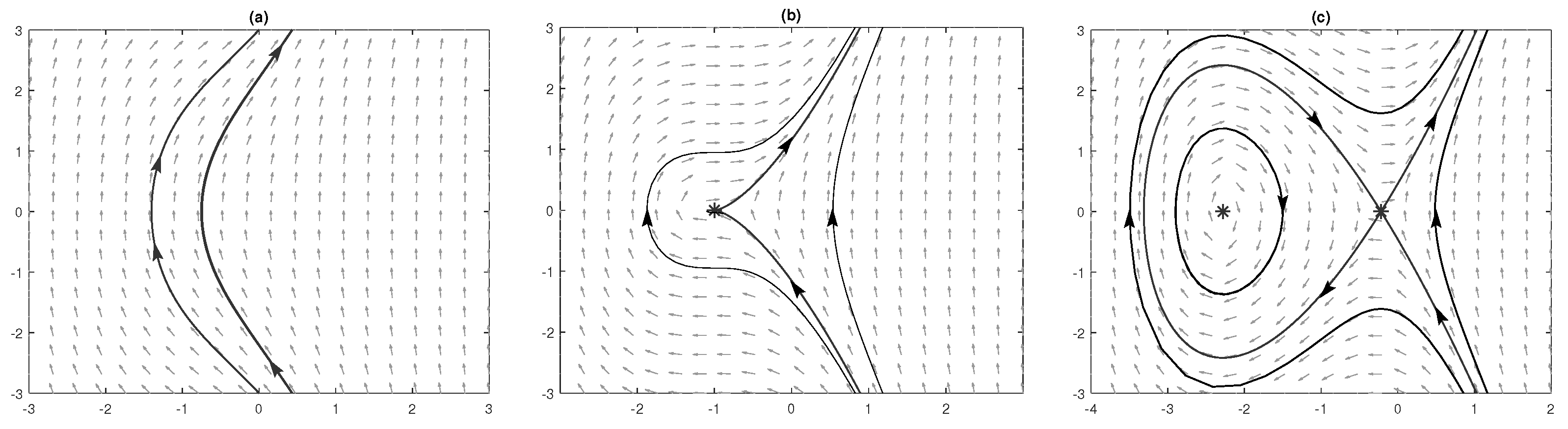
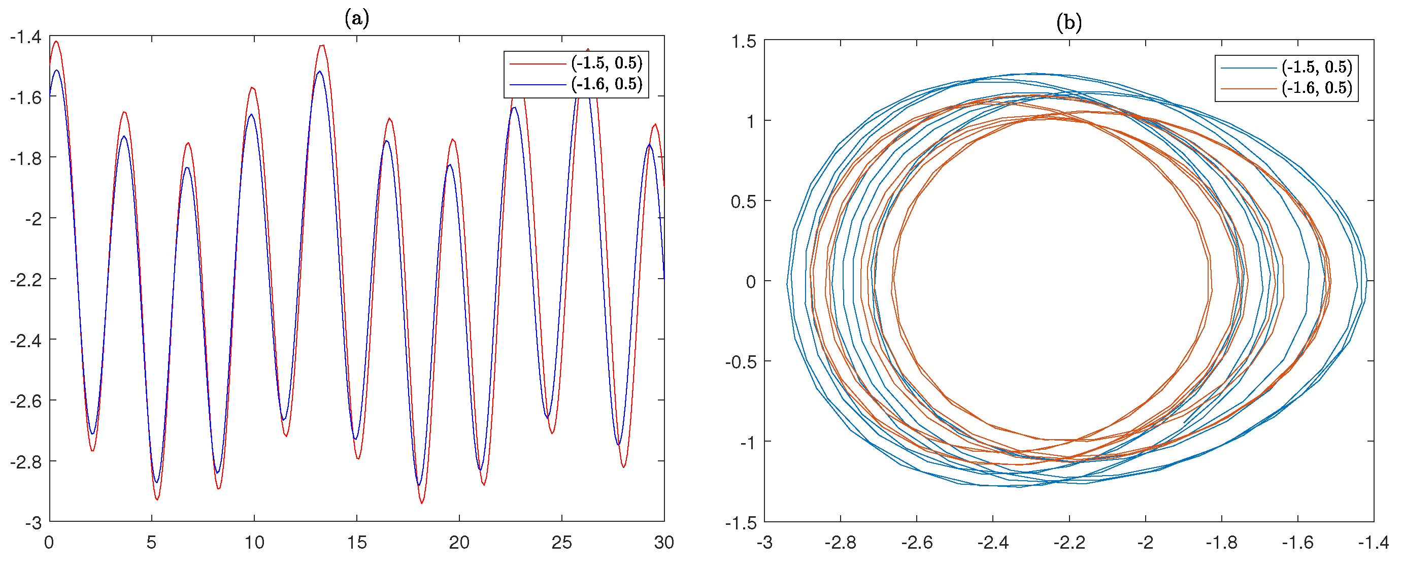
5. Dynamics Analysis

5.1. Dynamics Behavior of the (3+1)-Dimensional gSW Equation

By letting $w^{\prime }=v$, we convert Equation (16) into the following planar system:

$$\begin{array}{cc}\hfill w^{\prime }& =v,\hfill \\ \hfill v^{\prime }& ={\mu }_1{w}^2+{\mu }_{2}w+{\mu }_3,\hfill \end{array}$$

(18)

where ${\mu }_1={\displaystyle \frac{3}{k}},{\mu }_2={\displaystyle \frac{k\tau -l\varsigma }{k^{3}l}},{\mu }_3=-{\displaystyle \frac{c}{k^{3}l}}$. Then, system (18) is a Hamiltonian system with the Hamiltonian

$$H={\displaystyle \frac{1}{2}}{v}^2-{\displaystyle \frac{{\mu }_1}{3}}{w}^3-{\displaystyle \frac{{\mu }_2}{2}}{w}^2-{\mu }_{3}w.$$

The Jacobian of Equation (18) is

$$J(w,v)=\left|\begin{array}{cc}0& 1\\ 2{\mu }_{1}w+{\mu }_2& 0\end{array}\right|=-2{\mu }_{1}w-{\mu }_2.$$

We assume $\Delta ={\mu }_2^2-4{\mu }_1{\mu }_3$. Then, the equilibrium points of system (18) can be obtained as follows:

Case 1: If $\Delta <0$, system (18) has no equilibrium point.

Case 2: If $\Delta =0$, system (18) has a unique equilibrium point

$$(w_0,v_0)=\left({\displaystyle \frac{-{\mu }_2}{2{\mu }_1}},0\right).$$

Case 3: If $\Delta >0$, the equilibrium points of system (18) are

$$(w_1,v_1)=\left({\displaystyle \frac{-{\mu }_2-\sqrt{\Delta }}{2{\mu }_1}},0\right),(w_2,v_2)=\left({\displaystyle \frac{-{\mu }_2+\sqrt{\Delta }}{2{\mu }_1}},0\right).$$

Moreover, we can calculate the Jacobian of the equilibrium points as follows:

$$J(w_0,v_0)=0,J(w_1,v_1)=\sqrt{\Delta },J(w_2,v_2)=-\sqrt{\Delta }.$$

Hence, we conclude that the equilibrium point $(w_0,v_0)$ is a cuspid, the equilibrium points $(w_1,v_1)$ represent a center, and $(w_2,v_2)$ is a saddle.

We show the phase portraits of system (18) in Figure 1.

5.2. Chaos Behavior of the (3+1)-Dimensional gSW Equation

Chaotic dynamics describe the intricate, seemingly random patterns emerging from deterministic nonlinear systems governed by sensitive dependence on initial conditions. Within marine environments, surface wave interactions exhibit inherent chaotic properties due to nonlinear coupling between atmospheric forcing, bathymetric variations, and hydrodynamic instabilities. This understanding supports improved forecasting models for wave height modulation, rogue wave emergence, and long-term climate-driven pattern shifts. In this section, we explore the chaotic behavior of system (18) in case 3 under the influence of noise perturbations. The chaotic system is detailed as follows:

$$\begin{array}{cc}\hfill w^{\prime }& =v,\hfill \\ \hfill v^{\prime }& ={\mu }_1{w}^2+{\mu }_{2}w+{\mu }_3+f_{0}cos\left(\rho z\right),\hfill \end{array}$$

(19)

where ${\mu }_2^2-4{\mu }_1{\mu }_3>0$, $f_0$ is the amplitude of the external force, and $\rho$ is the frequency of the external force. Using this model, we analyze the sensitivity to noise in three aspects: amplitude, frequency, and initial conditions. We examine the effect of amplitude by varying $f_0$ while keeping $\rho$ and the initial conditions fixed. Similarly, the effect of frequency is studied by varying $\rho$ while keeping $f_0$ and the initial conditions fixed. Finally, the effect of initial conditions is analyzed by varying the starting values of $w\left(0\right)$ and $v\left(0\right)$ while keeping $f_0$ and $\rho$ constant. Simulations are presented using phase portraits and time series plots in Figure 2, Figure 3 and Figure 4, with parameters set to ${\mu }_1=2$, ${\mu }_2=5$, and ${\mu }_3=1$.

In Figure 2, the initial conditions are fixed at $w\left(0\right)=-1$ and $v\left(0\right)=0.1$, while the amplitude $f_0$ is varied. The frequency $\rho =1$ is kept constant, and the amplitude $f_0$ is set to 0, 0.1, and 0.5, represented by red, blue, and green lines, respectively. In Figure 3, the frequency $\rho$ is fixed while the initial conditions remain $w\left(0\right)=-1$ and $v\left(0\right)=0.1$. The red line corresponds to $f_0=0$, the blue line represents $f_0=0.5$ with $\rho =0.1$, and the green line shows $f_0=0.5$ with $\rho =0.5$. In Figure 4, the parameters are set to $f_0=0.5$ and $\rho =0.5$. The red line represents the initial conditions $w\left(0\right)=-1.5$ and $v\left(0\right)=0.5$, while the blue line corresponds to $w\left(0\right)=-1.6$ and $v\left(0\right)=0.5$. The results show that the system is sensitive to noise perturbations in three aspects. The amplitude, frequency, and initiation have a significant impact on the chaotic behavior of the system.

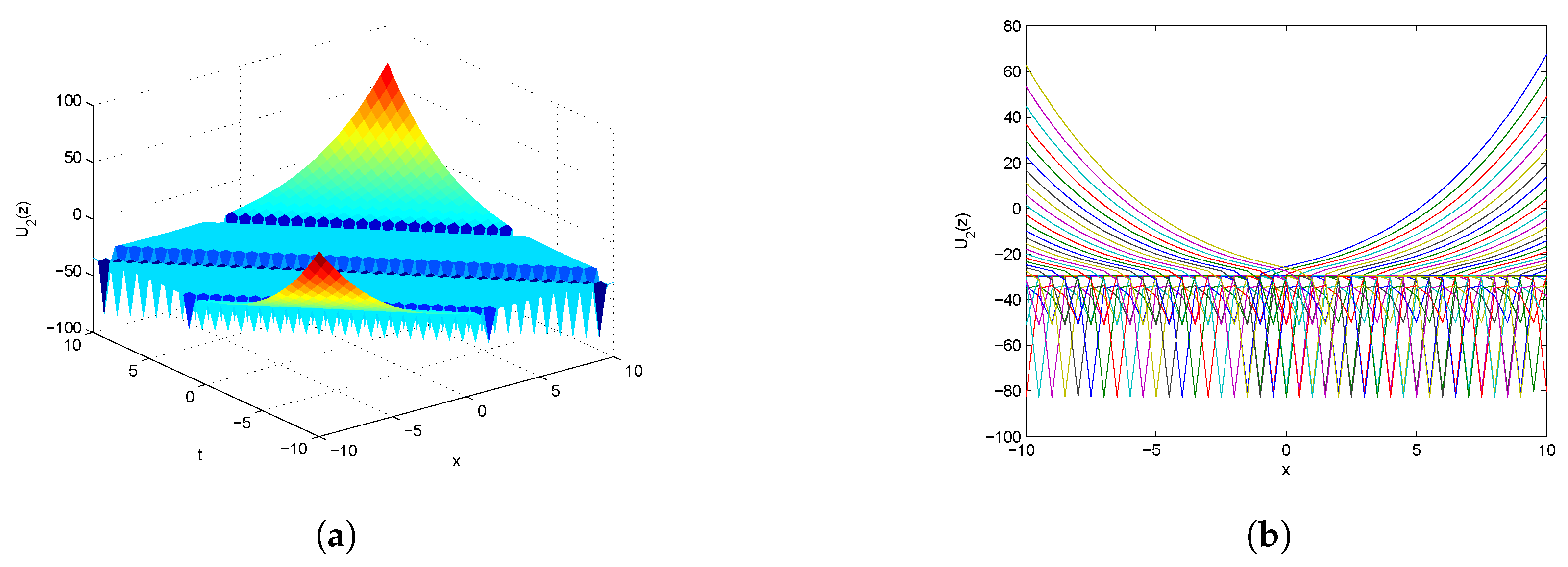
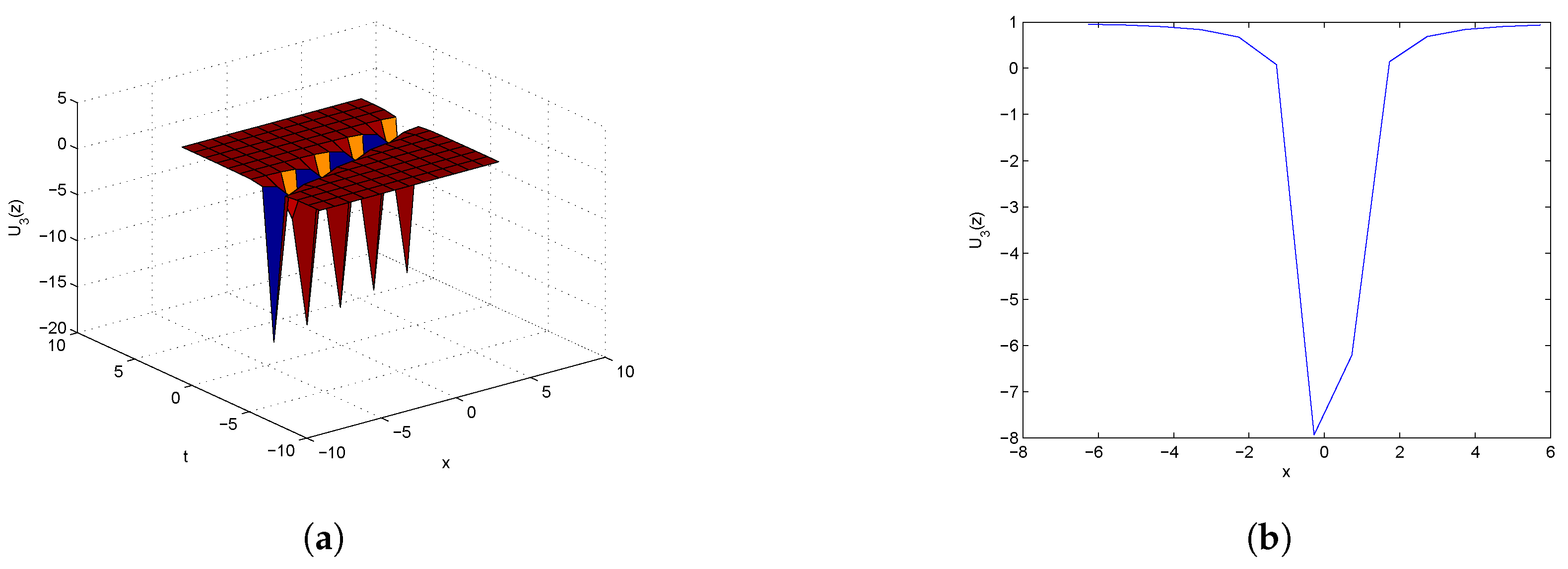
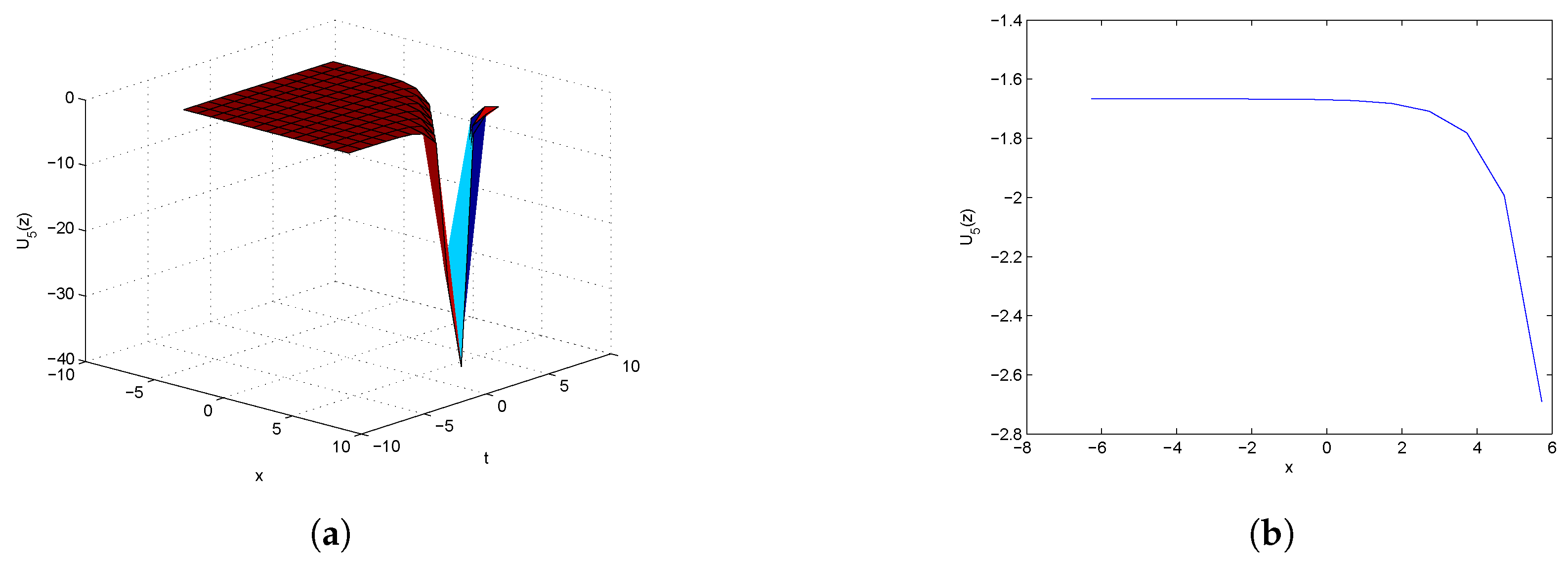
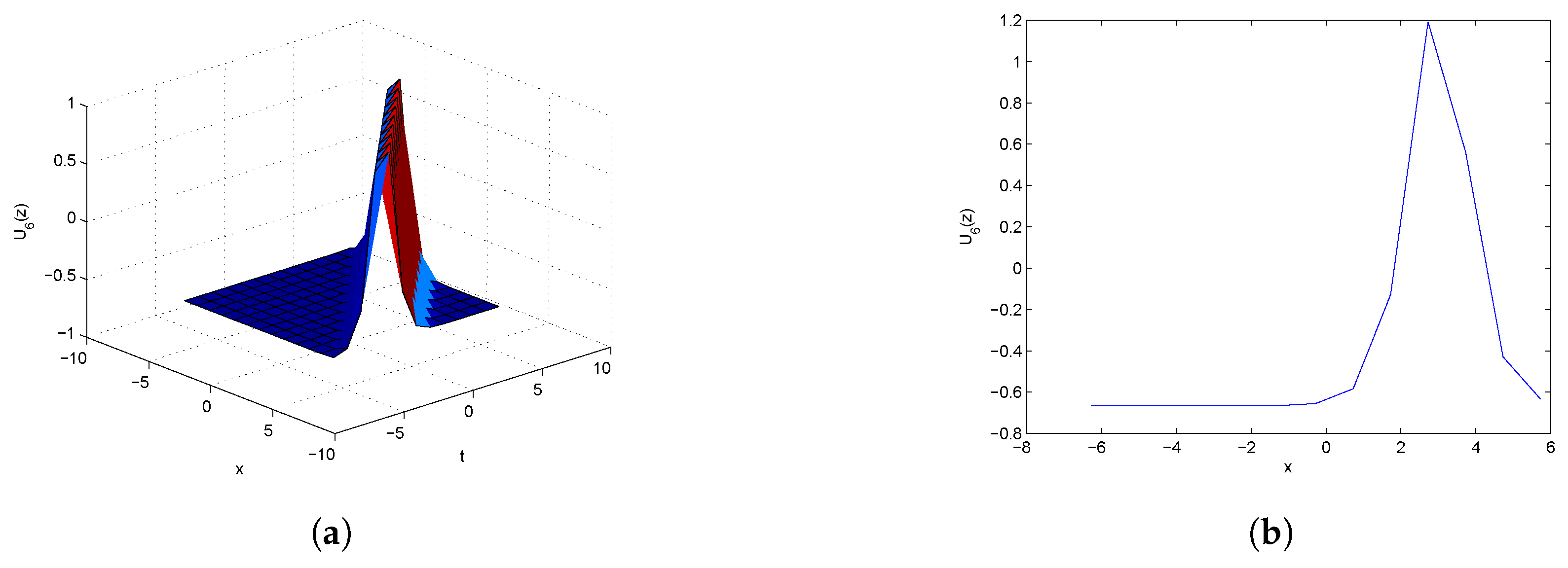
5.3. Dynamic Structure of the Solutions to the fSK Equation

This section presents a detailed visualization of the dynamic characteristics of the obtained solutions, with the aim of enhancing the comprehension of wave propagation patterns. Through graphical representations and computational analysis, we systematically examine the spatial and temporal evolution of the solution profiles. The visualization approach enables a deeper insight into the wave behavior, including its amplitude variations, phase transitions, and stability properties across different parameter regimes. Such an analysis facilitates the interpretation of complex wave interactions and provides valuable information about the system’s nonlinear dynamics.

By using Matlab Version 9.14.0.2306882 (R2023a) for computer simulation, we obtained 3D and 2D images of elliptic, hyperbolic, and rational function solutions of the fSK equation, which appear in the form of multiple dark solitons, dark solitons, and bright solitons. These soliton solutions have significant implications in many different fields. Of particular note is the bright soliton, which plays a crucial role in fiber optic communication systems. Its unique localized wave packet structure enables high-speed data transmission and significantly reduces signal distortion. On the other hand, the observation of dark solitons greatly facilitates the study of quantum processes, manifested as a decrease in strength in Bose–Einstein condensates [42].

The solutions are plotted using specific parameters to illustrate their dynamic structure. We depict elliptic solutions $U_1\left(z\right)$ in Figure 5 by setting $\lambda =-1$, $\omega =0.4$, $C=1$, $D=0.037$, $g_2=-0.194$, and $U_2\left(z\right)$ in Figure 6 by choosing the values $\lambda =-1$, $\omega =-1$, $C=1$, $D=0.037$, and $g_2=-0.194$. The profiles of rational solution $U_3\left(z\right)$ are shown in Figure 7 when choosing the values $\lambda =5$, $\omega =-15$, and $z_0=1$. The graphics of hyperbolic solutions are given in Figure 8 and Figure 9, respectively, when choosing the values $\lambda =1$, $\omega =1$, $\alpha =1$, and $z_0=8$ for $U_5\left(z\right)$ and setting the values $\lambda =1$, $\omega =1$, $\alpha =2$, and $z_0=3$ for $U_6\left(z\right)$.

6. Conclusions

In this paper, closed-form meromorphic solutions to the fSK equation and (3+1)-dimensional gSW equation are derived using the extended complex method. The solutions are in terms of elliptic, hyperbolic, rational, and exponential functions. The planar dynamics behavior of the (3+1)-dimensional gSW equation is analyzed. The phase portraits are shown. Furthermore, The chaos behaviors of the (3+1)-dimensional gSW equation under noise perturbations are examined by computational simulation. The results show that the system is sensitive to noise perturbations in amplitude, frequency, and initial conditions. The dynamic behaviors of hyperbolic, trigonometric, exponential, elliptic, and rational solutions to the fSK equation are exhibited using images. The profiles of the Weierstrass elliptic function solutions $U_1\left(z\right)$ and $U_2\left(z\right)$ are more interesting and relatively rare in the literature. The methodological framework developed in this study demonstrates significant extensibility to a broad spectrum of NLDEs encountered in dynamic systems theory and complex systems analysis.

References

1. Gu, Y.; Peng, L.; Huang, Z.; Lai, Y. Soliton, breather, lump, interaction solutions and chaotic behavior for the (2+1)-dimensional KPSKR equation. Chaos Soliton. Fract. 2024, 187, 115351. [Google Scholar] [CrossRef]
2. Gu, Y.; Zhang, X.; Huang, Z.; Peng, L.; Lai, Y.; Aminakbari, N. Soliton and lump and travelling wave solutions of the (3+1) dimensional KPB like equation with analysis of chaotic behaviors. Sci. Rep. 2024, 14, 20966. [Google Scholar] [CrossRef] [PubMed]
3. Liu, J. Lump-type solutions and interaction solutions for the (2+1)-dimensional generalized fifth-order KdV equation. Appl. Math. Lett. 2018, 86, 36–41. [Google Scholar] [CrossRef]
4. Liu, J.; Ye, Q. Stripe solitons and lump solutions for a generalized Kadomtsev-Petviashvili equation with variable coefficients in fluid mechanics. Nonlinear Dyn. 2019, 96, 23–29. [Google Scholar] [CrossRef]
5. Gu, Y.; Lai, Y. Analytical investigation of the fractional Klein-Gordon equation along with analysis of bifurcation, sensitivity and chaotic behaviors. Mod. Phys. Lett. B 2025, 39, 2550124. [Google Scholar] [CrossRef]
6. Seadawy, A.R.; Ali, K.K.; Liu, J. New optical soliton solutions for fokas-lenells dynamical equation via two various methods. Mod. Phys. Lett. B 2021, 35, 2150196. [Google Scholar] [CrossRef]
7. Baskonus, H.M.; Sulaiman, T.A.; Bulut, H. New solitary wave solutions to the (2+1)-dimensional Calogero-Bogoyavlenskii-Schiff and the Kadomtsev-Petviashvili hierarchy equations. Indian J. Phys. 2017, 135, 327–336. [Google Scholar] [CrossRef]
8. Baskonus, H.M.; Sulaiman, T.A.; Bulut, H. On the novel wave behaviors to the coupled nonlinear Maccari’s system with complex structure. Optik 2017, 131, 1036–1043. [Google Scholar] [CrossRef]
9. Hosseini, K.; Zabihi, A.; Samadani, F.; Ansari, R. New explicit exact solutions of the unstable nonlinear Schrödinger’s equation using the expa and hyperbolic function methods. Opt. Quant. Electron. 2018, 50, 82. [Google Scholar] [CrossRef]
10. Hosseini, K.; Manafian, J.; Samadani, F.; Foroutan, M.; Mirzazadeh, M.; Zhou, Q. Resonant optical solitons with perturbation terms and fractional temporal evolution using improved tan (ϕ(η)/2)-expansion method and exp function approach. Optik 2018, 158, 933–939. [Google Scholar] [CrossRef]
11. Hosseini, K.; Samadani, F.; Kumar, D.; Faridi, M. New optical solitons of cubic-quartic nonlinear Schrödinger equation. Optik 2018, 157, 1101–1105. [Google Scholar] [CrossRef]
12. Hosseini, K.; Yazdani Bejarbaneh, E.; Bekir, A.; Kaplan, M. New exact solutions of some nonlinear evolution equations of pseudoparabolic type. Opt. Quant. Electron. 2017, 49, 241. [Google Scholar] [CrossRef]
13. Ali, K.K.; Rezazadeh, H.; Talarposhti, R.A.; Bekir, A. New soliton solutions for resonant nonlinear Schródinger’s equation having full nonlinearity. Int. J. Mod. Phys. B 2020, 34, 2050032. [Google Scholar] [CrossRef]
14. Ali, K.K.; Wazwaz, A.M.; Mehanna, M.S.; Osman, M.S. On short-range pulse propagation described by (2+1)-dimensional Schródinger’s hyperbolic equation in nonlinear optical fibers. Phys. Scr. 2020, 95, 75203. [Google Scholar] [CrossRef]
15. Roshid, H.; Rahman, M. The exp(-ϕ(ξ))-expansion method with application in the (1+1)-dimensional classical Boussinesq equations. Results Phys. 2014, 4, 150–155. [Google Scholar] [CrossRef]
16. Khan, K.; Akbar, M. The exp(-ϕ(ξ))-expansion method for finding traveling wave solutions of Vakhnenko-Parkes equation. Int. J. Dyn. Syst. Differ. Equ. 2014, 5, 72–83. [Google Scholar]
17. Kadkhoda, N.; Jafari, H. Analytical solutions of the Gerdjikov-Ivanov equation by using exp(-φ(ξ))-expansion method. Optik 2017, 139, 72–76. [Google Scholar] [CrossRef]
18. Aminakbari, N.; Gu, Y.; Dang, G. Study on soliton behaviors of the complex nonlinear Fokas-Lenells equation utilizing different methods. Mod. Phys. Lett. B 2024, 38, 2450340. [Google Scholar] [CrossRef]
19. Gu, Y.; Jiang, C.; Lai, Y. Analytical Solutions of the fractional Hirota-Satsuma coupled KdV equation along with analysis of bifurcation, sensitivity and chaotic behaviors. Fractal Fract. 2024, 8, 585. [Google Scholar] [CrossRef]
20. Yuan, W.; Xiong, W.; Lin, J.; Wu, Y. All meromorphic solutions of an auxiliary ordinary differential equation and its applications. Acta Math. Sci. 2015, 35, 1241–1250. [Google Scholar] [CrossRef]
21. Yuan, W.; Meng, F.; Huang, Y.; Wu, Y. All traveling wave exact solutions Of the variant Boussinesq equations. Appl. Math. Comput. 2015, 268, 865–872. [Google Scholar] [CrossRef]
22. Gu, Y.; Yuan, W.; Aminakbari, N.; Lin, J. Meromorphic solutions of some algebraic differential equations related Painlevé equation IV and its applications. Math. Meth. Appl. Sci. 2018, 41, 3832–3840. [Google Scholar] [CrossRef]
23. Ye, F.; Tian, J.; Zhang, X.; Jiang, C.; Ouyang, T.; Gu, Y. All traveling wave exact solutions of the Kawahara equation using the complex method. Axioms 2022, 11, 330. [Google Scholar] [CrossRef]
24. Bergweiler, W.; Rippon, P.; Stallard, G. Dynamics of meromorphic functions with direct or logarithmic singularities. Proc. Lond. Math. Soc. 2008, 97, 368–400. [Google Scholar] [CrossRef]
25. Conte, R.; Ng, T.W.; Wu, C. Closed-form meromorphic solutions of some third order boundary layer ordinary differential equations. Bull. Sci. Math. 2022, 174, 103096. [Google Scholar] [CrossRef]
26. Eremenko, A. Meromorphic traveling wave solutions of the Kuramoto-Sivashinsky equation. J. Math. Phys. 2006, 2, 278–286. [Google Scholar]
27. Kudryashov, N.A. Meromorphic solutions of nonlinear ordinary differential equations. Commun. Nonlinear Sci. Numer. Simul. 2010, 15, 2778–2790. [Google Scholar] [CrossRef]
28. Kudryashov, N.A.; Sinelshchikov, D.I.; Demina, M.V. Exact solutions of the generalized Bretherton equation. Phys. Lett. A 2011, 375, 1074–1079. [Google Scholar] [CrossRef]
29. Yuan, W.; Li, Y.; Lin, J. Meromorphic solutions of an auxiliary ordinary differential equation using complex method. Math. Meth. Appl. Sci. 2013, 36, 1776–1782. [Google Scholar] [CrossRef]
30. Yuan, W.; Wu, Y.; Chen, Q.; Huang, Y. All meromorphic solutions for two forms of odd order algebraic differential equations and its applications. Appl. Math. Comput. 2014, 240, 240–251. [Google Scholar] [CrossRef]
31. Yuan, W.; Huang, Z.; Fu, M.; Lai, J. The general solutions of an auxiliary ordinary differential equation using complex method and its applications. Adv. Differ. Equ. 2014, 2014, 147. [Google Scholar] [CrossRef]
32. Sawada, K.; Kotera, T. A method for finding N-soliton solutions of the K.d.V. equation and K.d.V.-Like Equation. Progr. Theoret. Phys. 1974, 51, 1355–1367. [Google Scholar] [CrossRef]
33. Tang, Y.; Ma, W.; Xu, W. Grammian and Pfaffian solutions as well as Pfaffianization for a (3+1)-dimensional generalized shallow water equation. Chin. Phys. B 2012, 21, 070212. [Google Scholar] [CrossRef]
34. Liu, C.; Dai, Z. Exact soliton solutions for the fifth-order Sawada-Kotera equation. Appl. Math. Comput. 2008, 206, 272–275. [Google Scholar] [CrossRef]
35. Naher, H.; Abdullah, F.A.; Mohyud-Din, S.T. Extended generalized Riccati equation mapping method for the fifth-order Sawada-Kotera equation. AIP Adv. 2013, 3, 52104. [Google Scholar] [CrossRef]
36. Guo, Y.; Li, D.; Wang, J. The new exact solutions of the fifth-order Sawada-Kotera equation using three wave method. Appl. Math. Lett. 2019, 94, 232–237. [Google Scholar] [CrossRef]
37. Gu, J.; Zhang, Y.; Dong, H. Dynamic behaviors of interaction solutions of (3+1)-dimensional shallow water wave equation. Comput. Math. Appl. 2018, 76, 1408–1419. [Google Scholar] [CrossRef]
38. Kumar, S.; Kumar, D. Analytical soliton solutions to the generalized (3+1)-dimensional shallow water wave equation. Mod. Phys. Lett. B 2022, 36, 2150540. [Google Scholar] [CrossRef]
39. Shi, F.; Qi, M.; Wang, K. Multi-kink solitons, resonant soliton molecules and multi-lumps solutions to the (3+1)-dimensional shallow water wave equation. Mod. Phys. Lett. B 2025, 39, 2550039. [Google Scholar] [CrossRef]
40. Zhang, Y.; Dong, H.; Zhang, X.; Yang, H. Rational solutions and lump solutions to the generalized (3+1)-dimensional shallow water-like equation. Comput. Math. Appl. 2017, 73, 246–252. [Google Scholar] [CrossRef]
41. Lang, S. Elliptic Functions, 2nd ed.; Springer: New York, NY, USA, 1987. [Google Scholar]
42. Kivshar, Y.S.; Luther-Davies, B. Dark optical solitons: Physics and applications. Phys. Rep. 1998, 298, 81–197. [Google Scholar] [CrossRef]
Figure 1. The phase portraits of system (18) corresponding to (a) Δ < 0 , (b) Δ = 0 , and (c) Δ > 0 . The stars represent the equilibrium.
Axioms 14 00334 g001
Figure 2. Chaos analysis of system (19) with varying amplitude: (a) time series plot; (b) phase portrait.
Axioms 14 00334 g002
Figure 3. Chaos analysis of system (19) with varying frequency: (a) time series plot; (b) phase portrait.
Axioms 14 00334 g003
Figure 4. Chaos analysis of system (19) with varying initiation: (a) time series plot; (b) phase portrait.
Axioms 14 00334 g004
Figure 5. The 3D and 2D graphics of U 1 ( z ) when choosing the values λ = 1 , ω = 0.4 , C = 1 , D = 0.037 , g 2 = 0.194 , and t = 0 for the 2D graphic.
Axioms 14 00334 g005
Figure 6. The 3D and 2D graphics of U 2 ( z ) when choosing the values λ = 1 , ω = 1 , C = 1 , D = 0.037 , g 2 = 0.194 , and t = 0 for the 2D graphic.
Axioms 14 00334 g006
Figure 7. The 3D and 2D graphics of U 3 ( z ) when choosing the values λ = 5 , ω = 15 , z 0 = 1 , and t = 0 for the 2D graphic.
Axioms 14 00334 g007
Figure 8. The 3D and 2D graphics of U 5 ( z ) when choosing the values λ = 1 , ω = 1 , α = 1 , z 0 = 8 , and t = 0 for the 2D graphic.
Axioms 14 00334 g008
Figure 9. The 3D and 2D graphics of U 6 ( z ) when choosing the values λ = 1 , ω = 1 , α = 2 , z 0 = 3 , and t = 0 for the 2D graphic.
Axioms 14 00334 g009
Disclaimer/Publisher’s Note: The statements, opinions and data contained in all publications are solely those of the individual author(s) and contributor(s) and not of MDPI and/or the editor(s). MDPI and/or the editor(s) disclaim responsibility for any injury to people or property resulting from any ideas, methods, instructions or products referred to in the content.