Efficient BEM-Based Algorithm for Pricing Floating Strike Asian Barrier Options (with MATLAB^® Code)

Abstract

This paper aims to illustrate how SABO (Semi-Analytical method for Barrier Option pricing) is easily applicable for pricing floating strike Asian barrier options with a continuous geometric average. Recently, this method has been applied in the Black–Scholes framework to European vanilla barrier options with constant and time-dependent parameters or barriers and to geometric Asian barrier options with a fixed strike price. The greater efficiency of SABO with respect to classical finite difference methods is clearly evident in numerical simulations. For the first time, a user-friendly MATLAB^® code is made available here.

1. Introduction

The pricing of continuously-monitored Asian options is a relevant task from both a mathematical and a financial point of view.

Asian options are quite common derivatives because they provide protection against strong price fluctuations in volatile markets and reduce the possibilities of price manipulations. The payoff of an Asian option depends on the average price of the underlying asset that is less volatile than the asset price itself. In general, Asian options are hence less valuable than their vanilla European counterparts because an option on a lower volatility asset is worth less.

On the other hand, it is more difficult to deal with Asian options than vanilla options because their price depends on the average value assumed by the underlying asset during the option’s life, requiring some mathematical effort in order to describe the dynamics of the average under consideration.

In this paper, Asian options are equipped with a continuously-monitored geometric average [1]. Asian options evaluated with the geometric mean, although not common among practitioners, give some information also about the evaluation of Asian options with the arithmetic mean [2]. From a theoretical point of view, the method illustrated in the paper is extensible to arithmetic Asian options, as well, with slight modification, but from the numerical point of view, there are several problems that we plan to investigate in the near future. Defining the stochastic process

$$A_t:={\int }_0^{t}log\left(S_{\tau }\right)d\tau$$

(1)

then the geometric average is defined as $exp\left(\frac{A_t}{t}\right)$. When A and S are written with subscripts (A_t and S_t), they are intended as stochastic processes; otherwise, they are considered independent variables in the differential analysis context. The differential problem that describes the price evolution of this option is:

$$\begin{array}{cc}\hfill {\displaystyle \frac{\partial V}{\partial t}+\frac{{\sigma }^2}{2}{S}^2\frac{{\partial }^{2}V}{\partial S^2}+rS\frac{\partial V}{\partial S}+log\left(S\right)\frac{\partial V}{\partial A}-rV=0,}& S\in {\mathbb{R}}^{+},A\in \mathbb{R},t\in [0,T)\hfill \end{array}$$

(2)

$$\begin{array}{cc}\hfill {\displaystyle V(S,A,T)\mathrm{assigned},}& S\in {\mathbb{R}}^{+},A\in \mathbb{R}.\hfill \end{array}$$

(3)

Wanting to provide a further protection against excessive fluctuations of the strike price, it is possible to apply barriers in the option contract; for example, knock-out barriers make the option cease to exist if the underlying asset reaches a barrier during the life of the option. The model analyzed in this paper concerns an Asian option with an up-and-out barrier at $S=B$ and a floating strike payoff, i.e.,

$$\begin{array}{cc}\hfill {\displaystyle \frac{\partial V}{\partial t}+\frac{{\sigma }^2}{2}{S}^2\frac{{\partial }^{2}V}{\partial S^2}+rS\frac{\partial V}{\partial S}+log\left(S\right)\frac{\partial V}{\partial A}-rV=0,}& S\in (0,B),A\in \mathbb{R},t\in [0,T)\hfill \end{array}$$

(4)

$$\begin{array}{cc}\hfill {\displaystyle V(S,A,T)\mathrm{assigned},}& S\in (0,B),A\in \mathbb{R}\hfill \end{array}$$

(5)

$$\begin{array}{cc}\hfill {\displaystyle V(B,A,t)=0,}& A\in \mathbb{R},t\in [0,T)\hfill \end{array}$$

(6)

$$\begin{array}{cc}\hfill \mathrm{asymptotic}\mathrm{conditions}\mathrm{of}\mathrm{vanilla}\mathrm{option},& \left\{\right(S,A):S=0\vee A\to -\infty \vee A\to +\infty \},\hfill \end{array}$$

(7)

with the final condition:

$$\begin{array}{cc}\hfill \mathrm{call}& {\displaystyle V(S,A,T)=max\left(S-exp\left(\frac{A}{T}\right),0\right)\mathrm{or}}\hfill \end{array}$$

(8)

$$\begin{array}{cc}\hfill \mathrm{put}& {\displaystyle V(S,A,T)=max\left(exp\left(\frac{A}{T}\right)-S,0\right).}\hfill \end{array}$$

(9)

The problem (2)–(3) of pricing a floating strike Asian option with a continuous geometric average and without a barrier has a closed-form solution in the domain $(S,A,t)\in {\mathbb{R}}^{+}\times \mathbb{R}\times [0,T)$ that can be formulated either as the payoff expected value (also known as the Feynman–Kac formula):

$${\displaystyle V(S,A,t)={\int }_{-\infty }^{+\infty }{\int }_0^{B}V(\tilde{S},\tilde{A},T)G(S,A,t;\tilde{S},\tilde{A},T)d\tilde{S}d\tilde{A},}$$

(10)

with the transition probability density function G associated with the differential operator defined in Equation (4), which is known to be:

$$\begin{array}{ccc}G(S,A,t;\tilde{S},\tilde{A},\tilde{t})\hfill & =\hfill & \frac{\sqrt{3}H[\tilde{t}-t]}{\pi {\sigma }^2{(\tilde{t}-t)}^2}exp\{-\frac{2}{{\sigma }^2(\tilde{t}-t)}{log}^2\left(\frac{S}{\tilde{S}}\right)+\frac{6}{{\sigma }^2{(\tilde{t}-t)}^2}log\left(\frac{S}{\tilde{S}}\right)\left(A-\tilde{A}+(\tilde{t}-t)log\left(S\right)\right)\hfill \\ & -\hfill & \frac{6}{{\sigma }^2{(\tilde{t}-t)}^3}{\left(A-\tilde{A}+(\tilde{t}-t)log\left(S\right)\right)}^2-{\left(\frac{2r+{\sigma }^2}{2\sqrt{2}\sigma }\right)}^2(\tilde{t}-t)\}{\left(\frac{\tilde{S}}{S}\right)}^{\frac{2r-{\sigma }^2}{2{\sigma }^2}}\frac{1}{\tilde{S}},\hfill \end{array}$$

(11)

or (see [3]) through the formula:

$$\begin{array}{c}{\displaystyle V_{\mathrm{call}}(S,A,t)=S\mathcal{N}\left[d\right]-e^{\frac{A}{T}}{S}^{\frac{T-t}{T}}{e}^q\mathcal{N}\left[d-\frac{\sigma }{T}\sqrt{\frac{T^3-t^3}{3}}\right]}\hfill \\ {\displaystyle d=\frac{t(log\left(S\right)-\frac{A}{t})+(r+\frac{{\sigma }^2}{2})\frac{T^2-t^2}{2}}{\sigma \sqrt{\frac{T^3-t^3}{3}}}}\hfill \\ {\displaystyle q=\frac{(t-T)[6Tr(t+T)+(T-t)(2t+T){\sigma }^2]}{12T^2}}\hfill \end{array}$$

(12)

for the call option, where $\mathcal{N}[·]$ is the normal cumulative distribution function, and eventually, the put-call parity:

$$\begin{array}{c}{\displaystyle V_{\mathrm{call}}(S,A,t)-V_{\mathrm{put}}(S,A,t)=S-e^{\frac{A}{T}}{S}^{\frac{T-t}{T}}{e}^q.}\hfill \end{array}$$

(13)

Instead, when applying barriers, no closed-formulas are available. In this context, SABO is a Semi-Analytical method conceived of for the pricing of Barrier Options, and its milestones are resumed in Section 4.1. It is quite a general method, applicable also to fixed strike payoffs [4,5], put options [6], time-dependent parameters [7] and double barriers [8].

SABO is compared here with two Finite Difference (FD) methods chosen among the wide class of numerical methods at our disposal [9]. Equation (4) is proven to be hypo-elliptic [10,11,12], a property that guarantees a smooth solution and should benefit from approximations based on Taylor expansions. Anyway, SABO appears to be certainly more efficient looking at the results below.

2. Results

We have performed several simulations related to the pricing of a geometric call Asian option with a floating strike price and with an up-and-out barrier as modeled by the differential problem (4)–(8). Numerical results, some of which are displayed in the following, have been obtained by the MATLAB^® codes implementing the algorithms of SABO, FD1 and FD2 described in Section 4.1, Section 4.2.1 and Section 4.2.2, respectively. In Section 5 the SABO code is provided.

Example 1.

In this example, we use the finance parameters displayed in

Table 1. Floating strike up-and-out call option data.

B	T	r	$\mathit{\sigma }$
150	1	0.035	0.2

. The floating strike call option with an up-and-out barrier at $S=150=:B$ is evaluated at $t=0$ and $A=0$, truncating the A-domain at $A_{\min }=0$ and $A_{\max }=5$, in accordance with (20) and either (19) or (27).

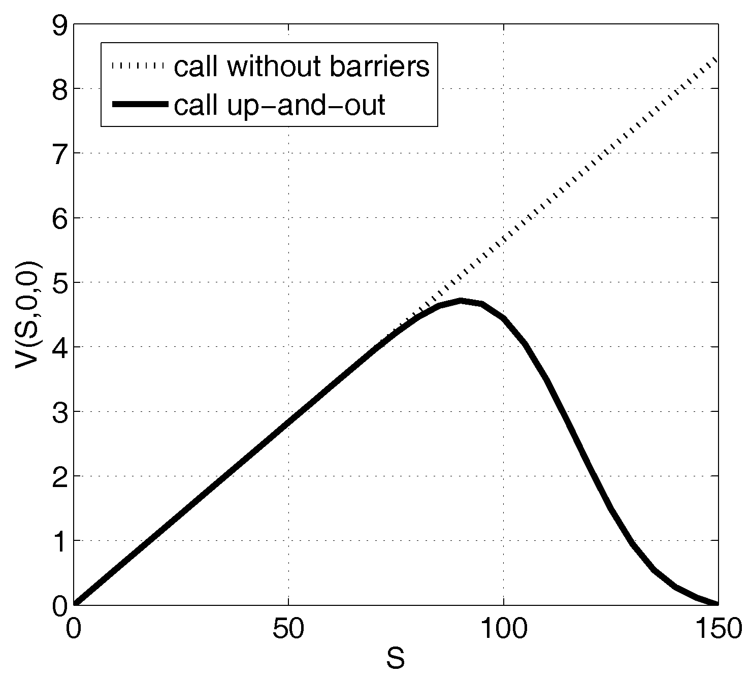
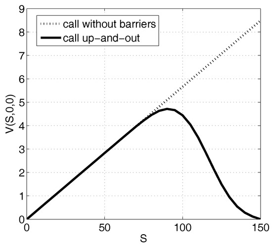
The approximation by SABO is obtained setting the parameters described in Section 4.1 $N_t=N_A=20$, and the option value is displayed in Figure 1 as a function of S.

The convergence at $S=100,120,140,148$ is shown in

Table 2. $V(S,0,0)$ evaluated by SABO at $S=100,120,140,148$.

${\mathit{N}}_{\mathit{t}}={\mathit{N}}_{\mathit{A}}$	$\mathit{S}=100$	$\mathit{S}=120$	$\mathit{S}=140$	$\mathit{S}=148$	Elapsed Time (s)
20	4.4059	2.1078	0.2771	0.0441	9.0 $\times {10}^0$
40	4.4339	2.2728	0.3814	0.0632	3.1 $\times {10}^1$
80	4.4335	2.3506	0.4683	0.0807	1.3 $\times {10}^2$
160	4.4334	2.3600	0.4854	0.0843	5.1 $\times {10}^2$
320	4.4333	2.3616	0.4882	0.0849	2.2 $\times {10}^3$
640	4.4333	2.3619	0.4887	0.0850	1.0 $\times {10}^4$

refining the mesh: at each level, parameters $N_t$ and $N_A$ are doubled.

The approximation by FD1 is obtained setting the discretization parameters (defined in (17), (18) and (30)) $\Delta t={10}^{-3}/2^k$, $\Delta A={10}^{-2}/2^k$ and, for the discretization of the asset domain $(0,B)$, either $\Delta S=2$ or $\Delta S=1$. The related results are reported in

Table 3. $V(S,0,0)$ evaluated by FD1at $S=100,120,140,148$, with $\Delta S=2$.

k	$\mathit{S}=100$	$\mathit{S}=120$	$\mathit{S}=140$	$\mathit{S}=148$	Elapsed Time (s)
1	5.8385	3.6788	0.9933	0.1834	6.9 $\times {10}^0$
2	5.2000	3.0951	0.7729	0.1405	3.3 $\times {10}^1$
3	4.8342	2.7511	0.6412	0.1148	1.5 $\times {10}^2$
4	4.6360	2.5610	0.5673	0.1004	5.3 $\times {10}^2$
5	4.5324	2.4605	0.5278	0.0926	2.1 $\times {10}^3$
6	4.4794	2.4087	0.5073	0.0886	8.5 $\times {10}^3$
7	4.4526	2.3824	0.4968	0.0866	4.1 $\times {10}^4$

and

Table 4. $V(S,0,0)$ evaluated by FD1 at $S=100,120,140,148$, with $\Delta S=1$.

k	$\mathit{S}=100$	$\mathit{S}=120$	$\mathit{S}=140$	$\mathit{S}=148$	Elapsed Time (s)
1	5.8427	3.6815	0.9946	0.1837	1.9 $\times {10}^1$
2	5.2047	3.0985	0.7744	0.1408	7.7 $\times {10}^1$
3	4.8392	2.7550	0.6429	0.1151	2.8 $\times {10}^2$
4	4.6413	2.5651	0.5691	0.1007	1.1 $\times {10}^3$
5	4.5380	2.4648	0.5296	0.0930	4.4 $\times {10}^3$
6	4.4551	2.4131	0.5092	0.0890	2.2 $\times {10}^4$
7	4.4583	2.3869	0.4988	0.0870	9.5 $\times {10}^4$

.

The approximation by FD2 is obtained setting the discretization parameters $\Delta t=\Delta A=0.01/2^k$ and either $\Delta S=2$ or $\Delta S=1$. The results are displayed in

Table 5. $V(S,0,0)$ evaluated by FD2 at $S=100,120,140,148$, with $\Delta S=2$.

k	$\mathit{S}=100$	$\mathit{S}=120$	$\mathit{S}=140$	$\mathit{S}=148$	Elapsed Time (s)
1	4.6607	2.5250	0.5016	0.0853	9.8 $\times {10}^0$
2	4.4796	2.3874	0.4806	0.0826	3.7 $\times {10}^1$
3	4.4394	2.3640	0.4845	0.0840	1.5 $\times {10}^2$
4	4.4296	2.3587	0.4861	0.0844	6.0 $\times {10}^2$
5	4.4269	2.3570	0.4864	0.0845	2.4 $\times {10}^3$
6	4.4261	2.3564	0.4864	0.0845	1.0 $\times {10}^4$

and

Table 6. $V(S,0,0)$ evaluated by FD2 at $S=100,120,140,148$, with $\Delta S=1$.

k	$\mathit{S}=100$	$\mathit{S}=120$	$\mathit{S}=140$	$\mathit{S}=148$	Elapsed Time (s)
1	4.6657	2.5287	0.5034	0.0857	2.8 $\times {10}^1$
2	4.4853	2.3918	0.4826	0.0831	1.2 $\times {10}^2$
3	4.4452	2.3685	0.4865	0.0844	4.5 $\times {10}^2$
4	4.4354	2.3632	0.4881	0.0848	1.9 $\times {10}^3$
5	4.4327	2.3616	0.4884	0.0849	7.6 $\times {10}^3$
6	4.4318	2.3609	0.4884	0.0849	4.8 $\times {10}^4$

.

Example 2.

In this example, we use the finance parameters displayed in

Table 7. Floating strike up-and-out call option data.

B	T	r
115	1	0.08

and volatility equal to $\sigma =0.2,0.3,0.4$. The floating strike call option with an up-and-out barrier at $S=115=:B$ is evaluated at $t=0$ and $A=0$, truncating the A-domain at $A_{\min }=0$ and $A_{\max }=5$, in accordance with (20) and (19).

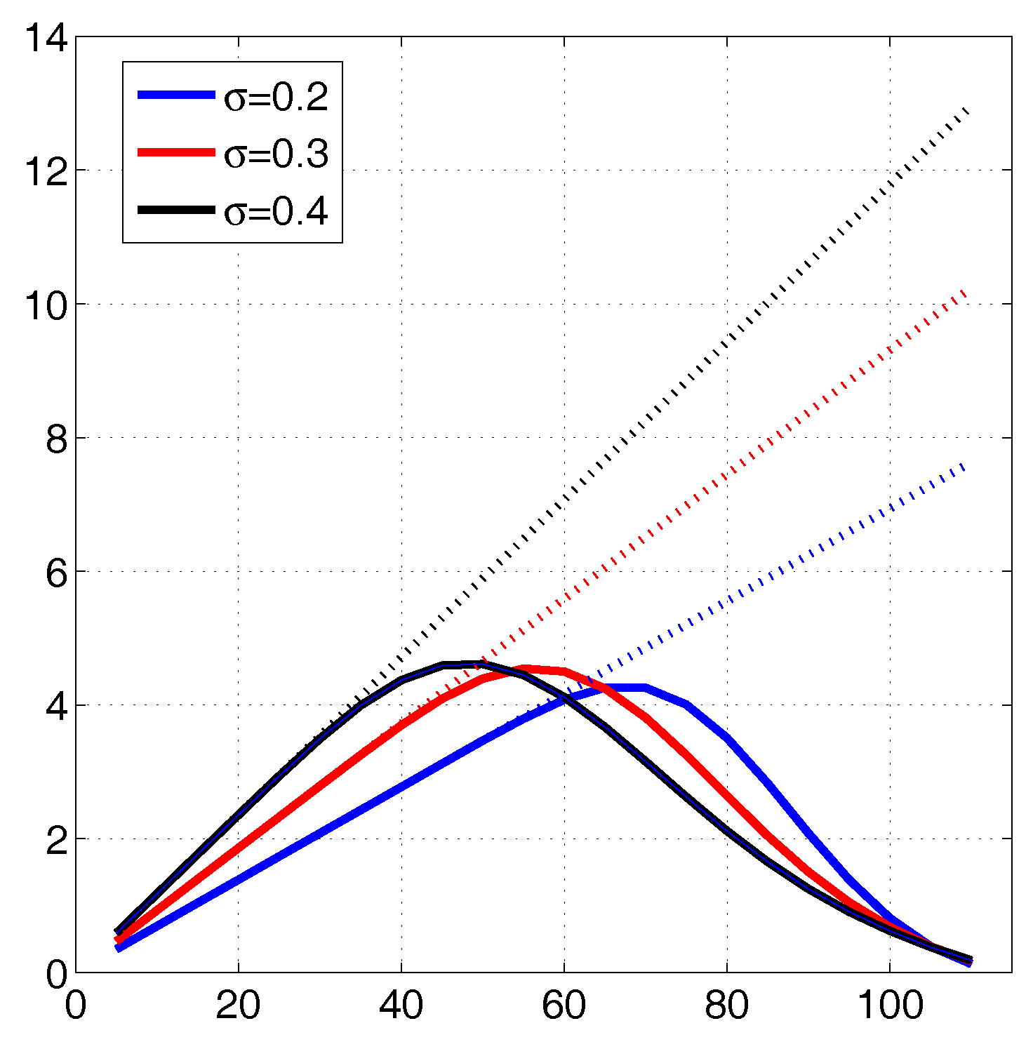
The approximation by SABO is obtained setting the parameters described in Section 4.1 $N_t=N_A=20$ and the option value is displayed in Figure 2 as a function of S for the different values of σ (continuous lines), in comparison with the corresponding prices of Asian options without barriers (dotted lines).

3. Discussion

Looking at Example 1, the values of a call option with an up-and-out barrier obtained by SABO and displayed in Figure 1 show that the solution, as expected, assumes lower values than the analogous option without barriers whose closed formula is (12) or that can be computed through the evaluation of the payoff expected value (10). The same behavior is recovered by the two proposed FD methods (FD1 and FD2).

Talking about efficiency and convergence, we have to look at the stabilization of the digits in Table 2, Table 3, Table 4, Table 5 and Table 6 where the option values at $S=100,120,140,148$ are written.

SABO, the results of which are written in Table 2, appears to be faster than the FD methods: doubling parameters $N_t$ and $N_A$, the CPU time for computation quadruples, but one more digit of accuracy is achieved. The convergence is slower near the barrier because there, the barrier option value is more different from the option value without barriers: the option value without the barrier can be quasi-exactly computed by the Feynman–Kac Formula (10), and therefore, the approximation error introduced by SABO solving the boundary integral Equation (15) related to the barrier case is more involved in representation Formula (14) as the asset nears the barrier (look at (26)).

Comparing Table 3 and Table 4, with an analogous computational time, SABO appears much more accurate and therefore efficient than FD1. Furthermore, note that FD1 is still sensitive to the mesh refinement in the S-domain: to halve $\Delta S$ means a significant variation in values of V together with a big increase of the computational costs.

Analyzing Table 5 and Table 6, we observe that FD2 has a superior accuracy compared to FD1 due to its higher order of consistency: approximations of derivatives in the t and A variables are both of second order. Anyway, FD2 is less efficient than SABO, and the coarseness of the S-grid still significantly affects its results. Refinements in the S-grid would result in much longer computational times, no longer comparable with those of SABO.

Looking at Example 2, SABO maintains its robustness varying the volatility values. The solutions displayed in Figure 2 show the property of smoothness proven in [11]. The increase in volatility causes the expected increase in the value of vanilla options, but on the contrary, it implies a diminishing of barrier option values near the barrier.

4. Methods

4.1. SABO

SABO is a Semi-Analytical method for the pricing of Barrier Options. The foundation on which it is based is the integral representation of the solution of the modeling differential problem based on the knowledge of the transition probability density function.

For a problem like that in (4)–(7), it is proven in [4] that the integral representation formula is: $\forall (S,A,t)\in (0,B)\times \mathbb{R}\times [0,T)$

$${\displaystyle V(S,A,t)={\int }_{-\infty }^{+\infty }{\int }_0^{B}V(\tilde{S},\tilde{A},T)G(S,A,t;\tilde{S},\tilde{A},T)d\tilde{S}d\tilde{A}+{\int }_t^T{\int }_{-\infty }^{+\infty }\frac{{\sigma }^2}{2}{B}^2\frac{\partial V}{\partial \tilde{S}}(B,\tilde{A},\tilde{t})G(S,A,t;B,\tilde{A},\tilde{t})d\tilde{A}d\tilde{t}}$$

(14)

where the transition probability density function $G(S,A,t;B,\tilde{A},\tilde{t})$ is defined in (11) and associated with the differential operator defined in Equation (4).

Note that in (14), both $V(S,A,t)$ and $\frac{\partial V}{\partial \tilde{S}}(B,\tilde{A},\tilde{t})$ are unknown, but, at $S=B$, the Boundary Condition (6) can be applied giving rise to the Volterra integral equation of the first kind:

$${\displaystyle 0=V(B,A,t)={\int }_{-\infty }^{+\infty }{\int }_0^{B}V(\tilde{S},\tilde{A},T)G(B,A,t;\tilde{S},\tilde{A},T)d\tilde{S}d\tilde{A}+{\int }_t^T{\int }_{-\infty }^{+\infty }\frac{{\sigma }^2}{2}{B}^2\frac{\partial V}{\partial \tilde{S}}(B,\tilde{A},\tilde{t})G(B,A,t;B,\tilde{A},\tilde{t})d\tilde{A}d\tilde{t}}$$

(15)

in the unknown $\frac{\partial V}{\partial \tilde{S}}(B,\tilde{A},\tilde{t})$.

The unknown is approximated by:

$${\displaystyle \frac{\partial V}{\partial \tilde{S}}(B,\tilde{A},\tilde{t})\approx \sum _{k=1}^{N_t}\sum _{h=1}^{N_A}{\alpha }_h^{\left(k\right)}{\psi }_h\left(\tilde{A}\right){\phi }_k\left(\tilde{t}\right)}$$

(16)

having defined piecewise constant basis functions:

$${\phi }_k\left(\tilde{t}\right):=H[\tilde{t}-t_{k-1}]-H[\tilde{t}-t_k],k=1,\dots ,N_t,$$

on a uniform time grid:

$${\displaystyle t_k:=k\Delta t,k=0,\dots ,N_t,\Delta t:=\frac{T}{N_t},N_t\in {\mathbb{N}}^{+},}$$

(17)

and piecewise constant basis functions:

$${\psi }_h\left(\tilde{A}\right):=H[\tilde{A}-A_{h-1}]-H[\tilde{A}-A_h],h=1,\dots ,N_A,$$

on a uniform A-grid over the truncated A-domain $[A_{min},A_{max}]$:

$${\displaystyle A_h:=A_{min}+h\Delta A,h=0,\dots ,N_A,\Delta A:=\frac{A_{max}-A_{min}}{N_A},N_A\in {\mathbb{N}}^{+}.}$$

(18)

A careful choice of $A_{min}$ and $A_{max}$ has to be performed in such a way that the double integral:

$${\int }_t^T{\int }_{-\infty }^{+\infty }G(B,A,t;B,\tilde{A},\tilde{t})d\tilde{A}d\tilde{t}$$

is rightly approximated by:

$${\int }_t^T{\int }_{A_{min}}^{A_{max}}G(B,A,t;B,\tilde{A},\tilde{t})d\tilde{A}d\tilde{t}.$$

By the analysis developed in [5], this results in seeking for $A_{\max }$ such that:

$$-{\int }_t^T\frac{exp\left(-\frac{(\tilde{t}-t){(2r+{\sigma }^2)}^2}{8{\sigma }^2}\right)}{2B\sigma \sqrt{2\pi (\tilde{t}-t)}}\mathrm{Erf}\left[\frac{\sqrt{6}\left(A-A_{\max }+(\tilde{t}-t)log\left(B\right)\right)}{{(\tilde{t}-t)}^{3/2}\sigma }\right]d\tilde{t}=\frac{\mathrm{Erf}\left[\frac{(2r+{\sigma }^2)\sqrt{T-t}}{2\sigma \sqrt{2}}\right]}{B(2r+{\sigma }^2)}$$

(19)

and $A_{\min }$ such that:

$${\int }_t^T\frac{exp\left(-\frac{(\tilde{t}-t){(2r+{\sigma }^2)}^2}{8{\sigma }^2}\right)}{2B\sigma \sqrt{2\pi (\tilde{t}-t)}}\mathrm{Erf}\left[\frac{\sqrt{6}\left(A-A_{\min }+(\tilde{t}-t)log\left(B\right)\right)}{{(\tilde{t}-t)}^{3/2}\sigma }\right]d\tilde{t}=\frac{\mathrm{Erf}\left[\frac{(2r+{\sigma }^2)\sqrt{T-t}}{2\sigma \sqrt{2}}\right]}{B(2r+{\sigma }^2)}$$

(20)

with a suitable tolerance. Otherwise, it is possible to consider the whole unbounded A-domain $\equiv \mathbb{R}$, but with two infinite basis functions, the first and the last, as investigated in [4].

In order to numerically solve the Volterra integral Equation (15), we convert it into a discrete linear system of equations by means of collocation BEM. Hence we collocate (15) at points:

$${\overline{A}}_i=\frac{A_i+A_{i-1}}{2},i=1,\dots ,N_A{\overline{t}}_j=\frac{t_j+t_{j-1}}{2},j=1,\dots ,N_t,$$

finally obtaining, for $i=1,\dots ,N_A,j=1,\dots ,N_t$:

$${\displaystyle {\int }_{{\overline{t}}_j}^T{\int }_{-\infty }^{+\infty }\frac{{\sigma }^2}{2}{B}^2\sum _{k=1}^{N_t}\sum _{h=1}^{N_A}{\alpha }_h^{\left(k\right)}{\psi }_h\left(\tilde{A}\right){\phi }_k\left(\tilde{t}\right)G(B,{\overline{A}}_i,{\overline{t}}_j;B,\tilde{A},\tilde{t})d\tilde{A}d\tilde{t}=-{\int }_{-\infty }^{+\infty }{\int }_0^{B}V(\tilde{S},\tilde{A},T)G(B,{\overline{A}}_i,{\overline{t}}_j;\tilde{S},\tilde{A},T)d\tilde{S}d\tilde{A}}$$

i.e., in matrix notation,

$$\mathcal{A}\alpha =\mathcal{F}.$$

(21)

The unknown vector is:

$$\alpha =\left({\alpha }^{\left(k\right)}{|}_{k=1,\dots ,N_t}\right)=\left(\left({\alpha }_h^{\left(k\right)}{|}_{h=1,\dots ,N_A}\right){|}_{k=1,\dots ,N_t}\right),$$

and the matrix entries are equal to the case of fixed strike Asian options deeply investigated also from a computational point of view in [4,5]: for $i,h=1,\dots ,N_A,j,k=1,\dots ,N_t$, define $\xi =i-h,\xi =-N_A+1,\dots ,N_A-1$ and $\ell =k-j,\ell =0,\dots ,N_t-1$, thus obtaining:

$$\begin{array}{ccc}\hfill {\displaystyle {\mathcal{A}}_{ih}^{\left(jk\right)}}& =& {\displaystyle \frac{\sigma B\Delta t}{4\sqrt{2\pi }}{\int }_{\frac{1}{2}-\frac{1}{2}H\left[\ell \right]}^1\frac{exp\left\{-{\left(\frac{2r+{\sigma }^2}{2\sqrt{2}\sigma }\right)}^2\Delta t(\tau +\ell -1/2)\right\}}{\sqrt{\Delta t(\tau +\ell -1/2)}}\left\{\mathrm{Erf}\left[\frac{\sqrt{6}\left(\Delta A(\xi +\frac{1}{2})+\Delta t(\tau +\ell -1/2)log\left(B\right)\right)}{\sigma \Delta t^{3/2}{(\tau +\ell -1/2)}^{3/2}}\right]\right.}\hfill \\ \hfill & -& {\displaystyle \left.\mathrm{Erf}\left[\frac{\sqrt{6}\left(\Delta A(\xi -\frac{1}{2})+\Delta t(\tau +\ell -1/2)log\left(B\right)\right)}{\sigma \Delta t^{3/2}{(\tau +\ell -1/2)}^{3/2}}\right]\right\}d\tau =:{\mathcal{A}}_{\xi }^{\left(\ell \right)}.}\hfill \end{array}$$

(22)

As we are considering constant coefficients in (4), the fundamental solution (11) depends on $t,\tilde{t},A,\tilde{A}$ only through the differences $t-\tilde{t}$ and $A-\tilde{A}$ implying that the matrix has a block-Toeplitz structure both in time and A-space:

$$\begin{array}{c}\mathcal{A}=\left[\begin{array}{ccccc}{\mathcal{A}}^{\left(0\right)}& {\mathcal{A}}^{\left(1\right)}& {\mathcal{A}}^{\left(2\right)}& \cdots & {\mathcal{A}}^{(N_t-1)}\\ 0& {\mathcal{A}}^{\left(0\right)}& {\mathcal{A}}^{\left(1\right)}& \cdots & {\mathcal{A}}^{(N_t-2)}\\ 0& 0& {\mathcal{A}}^{\left(0\right)}& \ddots & ⋮\\ ⋮& ⋮& \ddots & \ddots & {\mathcal{A}}^{\left(1\right)}\\ 0& 0& \cdots & 0& {\mathcal{A}}^{\left(0\right)}\end{array}\right]\\ \mathrm{with}{\mathcal{A}}^{\left(\ell \right)}=\left[\begin{array}{ccccc}{\mathcal{A}}_0^{\left(\ell \right)}& {\mathcal{A}}_{-1}^{\left(\ell \right)}& {\mathcal{A}}_{-2}^{\left(\ell \right)}& \cdots & {\mathcal{A}}_{-N_A+1}^{\left(\ell \right)}\\ {\mathcal{A}}_1^{\left(\ell \right)}& {\mathcal{A}}_0^{\left(\ell \right)}& {\mathcal{A}}_{-1}^{\left(\ell \right)}& \cdots & {\mathcal{A}}_{-N_A+2}^{\left(\ell \right)}\\ {\mathcal{A}}_2^{\left(\ell \right)}& {\mathcal{A}}_1^{\left(\ell \right)}& {\mathcal{A}}_0^{\left(\ell \right)}& \ddots & ⋮\\ ⋮& ⋮& \ddots & \ddots & {\mathcal{A}}_{-1}^{\left(\ell \right)}\\ {\mathcal{A}}_{N_A-1}^{\left(\ell \right)}& {\mathcal{A}}_{N_A-2}^{\left(\ell \right)}& \cdots & {\mathcal{A}}_1^{\left(\ell \right)}& {\mathcal{A}}_0^{\left(\ell \right)}\end{array}\right]\mathrm{for}\ell =0,\dots ,N_t-1\end{array}$$

(23)

so it is possible to adopt suitable strategies to save computational costs (as done in [13], even if this feature is not implemented in the code included here) and memory requirements.

A change in the payoff function is caught by the evaluation of the rhs entries: in the case of a floating strike call payoff, for $i=1,\dots ,N_A,j=1,\dots ,N_t$:

$$\begin{array}{ccc}\hfill {\mathcal{F}}_i^{\left(j\right)}& =& {\displaystyle -{\int }_{-\infty }^{+\infty }{\int }_0^{B}max\left(\tilde{S}-e^{\frac{\tilde{A}}{T}},0\right)G(B,{\overline{A}}_i,{\overline{t}}_j;\tilde{S},\tilde{A},T)d\tilde{S}d\tilde{A}}\hfill \end{array}$$

(24)

$$\begin{array}{cc}=& {\displaystyle \frac{B^{-\frac{2r-{\sigma }^2}{2{\sigma }^2}}}{2\sigma \sqrt{2\pi (T-{\overline{t}}_j)}}{\int }_0^B{\tilde{S}}^{\frac{2r-3{\sigma }^2}{2{\sigma }^2}+\frac{T-{\overline{t}}_j}{2T}}exp\left(-\frac{{(T-{\overline{t}}_j)}^2{(2r+{\sigma }^2)}^2+4{log}^2\left(\frac{B}{\tilde{S}}\right)}{8{\sigma }^2(T-{\overline{t}}_j)}\right)}\hfill \\ & {\displaystyle \left\{-{\tilde{S}}^{1-\frac{T-{\overline{t}}_j}{2T}}\mathrm{Erfc}\left[\sqrt{\frac{3}{2}}\frac{2{\overline{A}}_i+2(T-{\overline{t}}_j)log\left(B\right)-2Tlog\left(\tilde{S}\right)-(T-{\overline{t}}_j)log\left(\frac{B}{\tilde{S}}\right)}{\sigma {(T-{\overline{t}}_j)}^{\frac{3}{2}}}\right]\right.}\hfill \\ & {\displaystyle +B^{\frac{T-{\overline{t}}_j}{2T}}exp\left(\frac{{\overline{A}}_i}{T}+\frac{{\sigma }^2{(T-{\overline{t}}_j)}^3}{24T^2}\right)}\hfill \\ & {\displaystyle \left.\mathrm{Erfc}\left[\frac{12T{\overline{A}}_i+{\sigma }^2{(T-{\overline{t}}_j)}^3-6T\left(-2(T-{\overline{t}}_j)log\left(B\right)+2Tlog\left(\tilde{S}\right)+(T-{\overline{t}}_j)log\left(\frac{B}{\tilde{S}}\right)\right)}{2\sqrt{6}T\sigma {(T-{\overline{t}}_j)}^{\frac{3}{2}}}\right]\right\}d\tilde{S},}\hfill \end{array}$$

(25)

with $\mathrm{Erfc}$ the complementary of error function $\mathrm{Erf}$.

The approximation of $\frac{\partial V}{\partial \tilde{S}}(B,\tilde{A},\tilde{t})$ through the resolution of (21) is an intermediate step for the final evaluation of the option price by (14):

$$\begin{array}{ccc}\hfill V(S,A,t)& \approx & {\displaystyle -\frac{S^{-\frac{2r-{\sigma }^2}{2{\sigma }^2}}}{2\sigma \sqrt{2\pi (T-t)}}{\int }_0^B{\tilde{S}}^{\frac{2r-3{\sigma }^2}{2{\sigma }^2}+\frac{T-t}{2T}}exp\left(-\frac{{(T-t)}^2{(2r+{\sigma }^2)}^2+4{log}^2\left(\frac{S}{\tilde{S}}\right)}{8{\sigma }^2(T-t)}\right)}\hfill \\ & & {\displaystyle \left\{-{\tilde{S}}^{1-\frac{T-t}{2T}}\mathrm{Erfc}\left[\sqrt{\frac{3}{2}}\frac{2A+2(T-t)log\left(S\right)-2Tlog\left(\tilde{S}\right)-(T-t)log\left(\frac{S}{\tilde{S}}\right)}{\sigma {(T-t)}^{\frac{3}{2}}}\right]\right.}\hfill \\ & +& {\displaystyle S^{\frac{T-t}{2T}}exp\left(\frac{A}{T}+\frac{{\sigma }^2{(T-t)}^3}{24T^2}\right)}\hfill \\ & & {\displaystyle \left.\mathrm{Erfc}\left[\frac{12TA+{\sigma }^2{(T-t)}^3-6T\left(-2(T-t)log\left(S\right)+2Tlog\left(\tilde{S}\right)+(T-t)log\left(\frac{S}{\tilde{S}}\right)\right)}{2\sqrt{6}T\sigma {(T-t)}^{\frac{3}{2}}}\right]\right\}d\tilde{S}}\hfill \\ & +& {\displaystyle \frac{\sigma B}{4\sqrt{2\pi }}{\left(\frac{B}{S}\right)}^{\frac{2r-{\sigma }^2}{2{\sigma }^2}}\sum _{k=\mathrm{floor}\left[\frac{t}{\Delta t}\right]+1}^{N_t}\sum _{h=1}^{N_A}{\alpha }_h^{\left(k\right)}{\int }_{max(t,t_{k-1})}^{t_k}\frac{1}{\sqrt{\tilde{t}-t}}exp\left(-\frac{{(\tilde{t}-t)}^2{(2r+{\sigma }^2)}^2+4{log}^2\left(\frac{S}{B}\right)}{8(\tilde{t}-t){\sigma }^2}\right)}\hfill \\ & & {\displaystyle \left\{\mathrm{Erf}\left[\sqrt{\frac{3}{2}}\frac{2(A_h-A)-2(\tilde{t}-t)log\left(S\right)+(\tilde{t}-t)log\left(\frac{S}{B}\right)}{{(\tilde{t}-t)}^{3/2}\sigma }\right]\right.}\hfill \\ & -& {\displaystyle \left.\mathrm{Erf}\left[\sqrt{\frac{3}{2}}\frac{2(A_{h-1}-A)-2(\tilde{t}-t)log\left(S\right)+(\tilde{t}-t)log\left(\frac{S}{B}\right)}{{(\tilde{t}-t)}^{3/2}\sigma }\right]\right\}d\tilde{t}.}\hfill \end{array}$$

(26)

4.2. Finite Difference Methods

SABO is compared here (as in [5]) with two Finite Difference (FD) methods chosen among the wide class of FD methods available and deeply analyzed in [14]. This is because Equation (4) is proven to be hypoelliptic [10,11,12], a property that guarantees a smooth solution and that should benefit from approximations based on Taylor expansions.

The existence of the solution of Problem (4)–(5) and its Feynman–Kac representation (10) are proven involving stochastic arguments without the need for exact boundary conditions. Boundary conditions at $S=0$ and for $A\to \pm \infty$ have to be empirically deduced analogously to what was done in [5,15]. At $S=B$, Condition (6) holds.

In order to apply FD methods, the first step is to shrink to a bounded domain $[0,B]\times [A_{\min },A_{\max }]$ enclosing the option evaluation point $(S^{*},A^{*})$ and then apply boundary conditions at the borders.

• We have chosen $A_{\min }$ less than or equal to the minimum between the value suggested in (20) and $A^{*}$. There is not a consistent condition valid at $A=-\infty$ in finance, and as a consequence, it is not easy to conceive of a proper condition at points $(S,A_{\min },t)$. The use of the upwind method makes this condition unnecessary if $log\left(S\right)>0$ (as in the herein proposed examples). In fact, $\frac{\partial V}{\partial A}$ is approximated by a forward difference so that the boundary condition at $A_{\min }$ becomes useless; otherwise, if $log\left(S\right)<0$, a backward difference can be considered together with a condition on the derivative at $A=A_{\min }$, as for example $\frac{{\partial }^{2}V}{\partial A^2}(S,A_{\min },t)=0$.
• The upper bound is set at:

  $$A_{\max }=Tlog\left(B\right),$$

  (27)

  the maximum value assumed by the stochastic process $A_t$ defined in (1) if $S_t=B$ during the whole time interval $[0,T]$.
  The average $exp(A/T)$ is a non-decreasing function of time; therefore, if $exp(A/t)-B>0$ at time t, then $exp(A/T)-B>0$ at maturity, and so, the option is worth nothing as shown by the Payoff Function (8). Hence, if $log\left(S\right)>0$, $\frac{\partial V}{\partial A}$ is approximated by a forward difference and the boundary condition at $A_{\max }$ is set:

  $$V(S,A_{\max },t)=0.$$

  (28)
• At $S=0$, Equation (4) is degenerate, but if the stochastic process $S_t=0$ at any time, then the average asset price $exp(A_t/t)=constant$ and the option value V can be considered as independent of stochastic variables S and A, deducing from Equation (4) that:

  $$\underset{S\to 0}{lim}\left[\frac{\partial V}{\partial t}+\frac{{\sigma }^2}{2}{S}^2\frac{{\partial }^{2}V}{\partial S^2}+rS\frac{\partial V}{\partial S}+log\left(S\right)\frac{\partial V}{\partial A}-rV\right]=\underset{S\to 0}{lim}\left[\frac{\partial V}{\partial t}-rV\right]=0.$$
  The ordinary differential equation:

  $$\underset{S\to 0}{lim}\left[\frac{\partial V}{\partial t}-rV\right]=0$$

  suggests the condition:

  $$\underset{S\to 0}{lim}V(S,A,t)=e^{-r(T-t)}\underset{S\to 0}{lim}V(S,A,T)=0.$$

  (29)

The second step, after the definition of the computational domain, is the definition of the grid. Using a $(A,t)$-grid as defined by (17) and (18) in $[A_{\min },A_{\max }]\times [0,T]$, let us further introduce the S-grid in $[0,B]$:

$$\begin{array}{c}{\displaystyle \Delta S:=\frac{B}{N_S},N_S\in {\mathbb{N}}^{+},S_i:=i\Delta S,i=0,\dots ,N_S}\hfill \end{array}$$

(30)

and define the approximated option value:

$$V_{i,h}^k:\approx V(S_i,A_h,t_k).$$

• The values $V_{ih}^{N_t}$ can be found from the final condition:

  $$V_{i,h}^{N_t}=V(S_i,A_h,T),i=0,\cdots ,N_S-1,h=0,\cdots ,N_A;$$
• in the herein proposed examples, $log\left(S_i\right)>0$, so everywhere, we apply a forward difference and, at the boundary $A=A_{\max }$, Condition (28):

  $$V_{i,N_A}^k=0\mathrm{for}k=0,\cdots ,N_t-1,i=0,\cdots ,N_S-1;$$
• at the boundary $S=0$, we apply Condition (29):

  $$V_{0,h}^k=0h=0,\cdots ,N_A-1,k=0,\cdots ,N_t-1;$$
• at the boundary $S=B$, we apply the Boundary Condition (6), hence:

  $$V_{N_S,h}^k=0,h=0,\cdots ,N_A,k=0,\cdots ,N_t.$$

4.2.1. Finite Difference Method FD1

The first scheme FD1 is the very classical FD scheme where the derivatives of V in (4) are approximated by truncations of Taylor expansions:

• first order backward difference for the time derivative approximation:

  $$\frac{\partial V}{\partial t}(S_i,A_h,t_k)=\frac{V_{i,h}^k-V_{i,h}^{k-1}}{\Delta t}+O(\Delta t)$$
• second order central difference for the S derivative approximation:

  $$\frac{\partial V}{\partial S}(S_i,A_h,t_k)=\frac{V_{i+1,h}^k-V_{i-1,h}^k}{2\Delta S}+O(\Delta S^2)$$
• second order central difference for the S second order derivative approximation:

  $$\frac{{\partial }^{2}V}{\partial S^2}(S_i,A_h,t_k)=\frac{V_{i+1,h}^k-2V_{i,h}^k+V_{i-1,h}^k}{\Delta S^2}+O(\Delta S^2)$$
• if $log\left(S_i\right)>0$, first order forward difference for the A derivative approximation:

  $$\frac{\partial V}{\partial A}(S_i,A_h,t_k)=\frac{V_{i,h+1}^k-V_{i,h}^k}{\Delta A}+O(\Delta A)$$

We can now write down the discrete approximation of (4) at each point $(S_i,A_h,t_k)$:

for $i=1,\dots ,N_S-1,h=0,\dots ,N_A-1,k=0,\dots ,N_t-1$,

$$\frac{V_{i,h}^k-V_{i,h}^{k-1}}{\Delta t}+\frac{1}{2}{\sigma }^2{S}_i^2\frac{V_{i+1,h}^k-2V_{i,h}^k+V_{i-1,h}^k}{\Delta S^2}+r{S}_i\frac{V_{i+1,h}^k-V_{i-1,h}^k}{2\Delta S}+log\left(S_i\right)\frac{V_{i,h+1}^k-V_{i,h}^k}{\Delta A}-r{V}_{i,h}^k=0$$

(31)

and rearrange the scheme in a compact form:

$$V_{i,h}^{k-1}=a_i{V}_{i,h}^k+b_i{V}_{i+1,h}^k+c_i{V}_{i-1,h}^k+d_i{V}_{i,h+1}^k$$

where:

$$\begin{array}{c}{a}_i=1-\Delta t\left(r+{\sigma }^2{i}^2+\frac{log\left(S_i\right)}{\Delta A}\right),b_i=\frac{\Delta t}{2}\left(ri+{\sigma }^2{i}^2\right),c_i=\frac{\Delta t}{2}\left(-ri+{\sigma }^2{i}^2\right),d_i=\frac{\Delta t}{\Delta A}log\left(S_i\right).\hfill \end{array}$$

It is easy to see that the scheme, backward computing the new value $V_{i,h}^{k-1}$, is explicit in time.

We want to remark about two more things: first, the weights depend only on i, therefore on the S variable, and second, the values $V_{i,0}^k$ having $A_{\min }$ as the coordinate give no contribution to the scheme.

4.2.2. Finite Difference Method FD2

The method FD2 is suggested in [16]. The PDE (4) is collocated at the points:

$$(S_i,A_{h+\frac{1}{2}},t_{k+\frac{1}{2}}):=\left(S_i,A_h+\frac{\Delta A}{2},t_k+\frac{\Delta t}{2}\right).$$

Then, we use the following approximations, based on suitable Taylor expansions and standard finite difference approximations:

$$\begin{array}{ccc}\hfill \frac{\partial V}{\partial t}(S_i,A_{h+\frac{1}{2}},t_{k+\frac{1}{2}})& =& \frac{1}{2}\left(\frac{\partial V}{\partial t}(S_i,A_h,t_{k+\frac{1}{2}})+\frac{\partial V}{\partial t}(S_i,A_{h+1},t_{k+\frac{1}{2}})\right)+O(\Delta A^2)\hfill \\ & =& \frac{V_{i,h}^{k+1}-V_{i,h}^k}{2\Delta t}+\frac{V_{i,h+1}^{k+1}-V_{i,h+1}^k}{2\Delta t}+O(\Delta t^2+\Delta A^2),\hfill \end{array}$$

$$\begin{array}{ccc}\hfill \frac{\partial V}{\partial S}(S_i,A_{h+\frac{1}{2}},t_{k+\frac{1}{2}})& =& \frac{1}{2}\left(\frac{\partial V}{\partial S}(S_i,A_{h+1},t_{k+1})+\frac{\partial V}{\partial S}(S_i,A_h,t_k)\right)+O(\Delta t^2+\Delta A^2)\hfill \\ & =& \frac{V_{i+1,h+1}^{k+1}-V_{i-1,h+1}^{k+1}}{4\Delta S}+\frac{V_{i+1,h}^k-V_{i-1,h}^k}{4\Delta S}+O(\Delta t^2+\Delta A^2+\Delta S^2),\hfill \end{array}$$

$$\begin{array}{ccc}\frac{{\partial }^{2}V}{\partial S^2}(S_i,A_{h+\frac{1}{2}},t_{k+\frac{1}{2}})\hfill & =\hfill & \frac{1}{2}\left(\frac{{\partial }^{2}V}{\partial S^2}(S_i,A_{h+1},t_{k+1})+\frac{{\partial }^{2}V}{\partial S^2}(S_i,A_h,t_k)\right)+O(\Delta t^2+\Delta A^2)\hfill \\ & =\hfill & \frac{V_{i-1,h+1}^{k+1}-2V_{i,h+1}^{k+1}+V_{i+1,h+1}^{k+1}}{2\Delta S^2}+\frac{V_{i-1,h}^k-2V_{i,h}^k+V_{i+1,h}^k}{2\Delta S^2}+O(\Delta t^2+\Delta A^2+\Delta S^2),\hfill \end{array}$$

(32)

$$\begin{array}{ccc}\hfill V(S_i,A_{h+\frac{1}{2}},t_{k+\frac{1}{2}})& =& \frac{1}{2}\left(V_{i,h}^k+V_{i,h+1}^{k+1}\right)+O(\Delta t^2+\Delta A^2),\hfill \end{array}$$

$$\begin{array}{ccc}\hfill \frac{\partial V}{\partial A}(S_i,A_{h+\frac{1}{2}},t_{k+\frac{1}{2}})& =& \frac{1}{2}\left(\frac{\partial V}{\partial A}(S_i,A_{h+\frac{1}{2}},t_{k+1})+\frac{\partial V}{\partial A}(S_i,A_{h+\frac{1}{2}},t_k)\right)+O(\Delta t^2)\hfill \\ & =& \frac{V_{i,h+1}^{k+1}-V_{i,h}^{k+1}}{2\Delta A}+\frac{V_{i,h+1}^k-V_{i,h}^k}{2\Delta t}+O(\Delta t^2+\Delta A^2).\hfill \end{array}$$

After substituting the above approximations into the PDE and discarding the error terms, we get the following equations for the approximate values of the option prices:

$${\overline{a}}_i{V}_{i-1,h}^k+{\overline{b}}_i{V}_{i,h}^k+{\overline{c}}_i{V}_{i+1,h}^k={\overline{d}}_i{V}_{i-1,h+1}^{k+1}+{\overline{e}}_i{V}_{i,h+1}^{k+1}+{\overline{f}}_i{V}_{i+1,h+1}^{k+1}+{\overline{g}}_i(V_{i,h+1}^k-V_{i,h}^{k+1})$$

(33)

where, using the notation $\lambda =\frac{\Delta t}{\Delta S^2}$:

$$\begin{array}{c}{\overline{a}}_i=\frac{\lambda }{2}\left(-S_i^2{\sigma }^2+r{S}_i\Delta S\right),{\overline{b}}_i=\left(1+\lambda S_i^2{\sigma }^2+\frac{log\left(S_i\right)\Delta t}{\Delta A}+r\Delta t\right),{\overline{c}}_i=-\frac{\lambda }{2}\left(S_i^2{\sigma }^2+r{S}_i\Delta S\right),\hfill \\ {\overline{d}}_i=-a_i,{\overline{e}}_i=\left(1-\lambda S_i^2{\sigma }^2+\frac{log\left(S_i\right)\Delta t}{\Delta A}-r\Delta t\right),{\overline{f}}_i=-c_i,{\overline{g}}_i=\left(-1+\frac{log\left(S_i\right)\Delta t}{\Delta A}\right).\hfill \end{array}$$

The procedure for solving the option pricing equation is as follows:

(1)

Fill the values $V_{i,h}^{N_t},i=0,\cdots ,N_S,h=0,\cdots ,N_A$ using the payoff function.

(2)

For each $k=N_t-1:-1:0$:

(a)

Apply the boundary condition at $A=A_{\max }$ to define $V_{i,N_A}^k$, for $i=0,\cdots ,N_S$.

(b)

For each $h=N_A-1:-1:0$, solve for the three-diagonal system in the unknowns the values $V_{i,h}^k$, for $i=1,\cdots ,N_S-1$, using the boundary condition at $S=0$ and $S=B$.

This is a time-explicit difference scheme, as well. If we need the option price only at $t=0$, then it is not necessary to store the full matrix V of approximate option prices; in fact, we need only two levels, say $V_{old}$ corresponding to $t=t_{k+1}$ and $V_{new}$ corresponding to the current time level $t=t_k$. At the beginning, $V_{old}$ is computed using the final condition, and at the end of each time step, the values of $V_{new}$ are copied to $V_{old}$. Anyway, it requires the resolution of a linear system: the three-diagonal matrix $M=diag(\overline{a},\overline{b},\overline{c})$ can be assembled and factorized at the beginning, outside the cycles, depending only on the S-grid.

5. MATLAB^® Code Implementing SABO

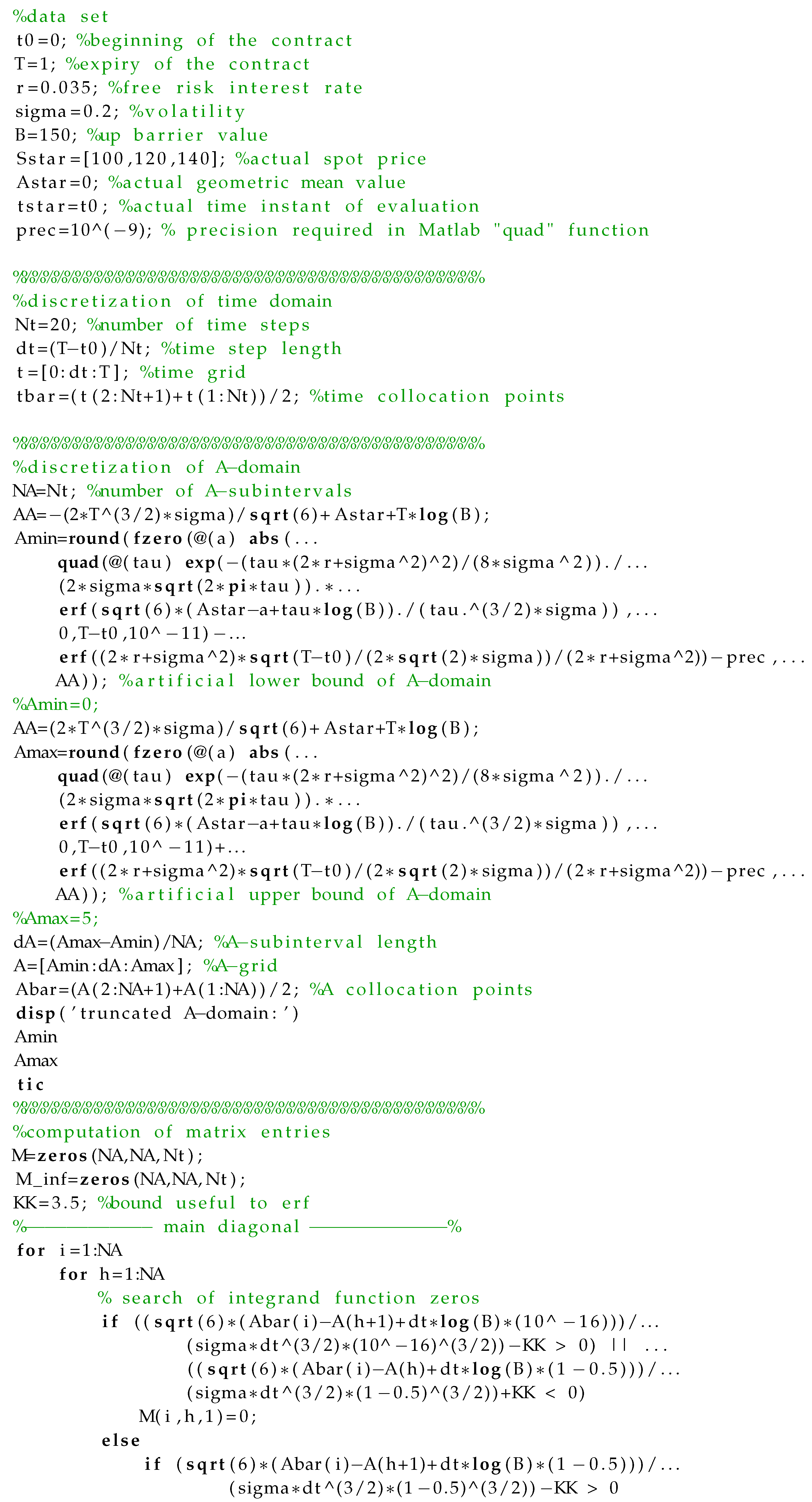
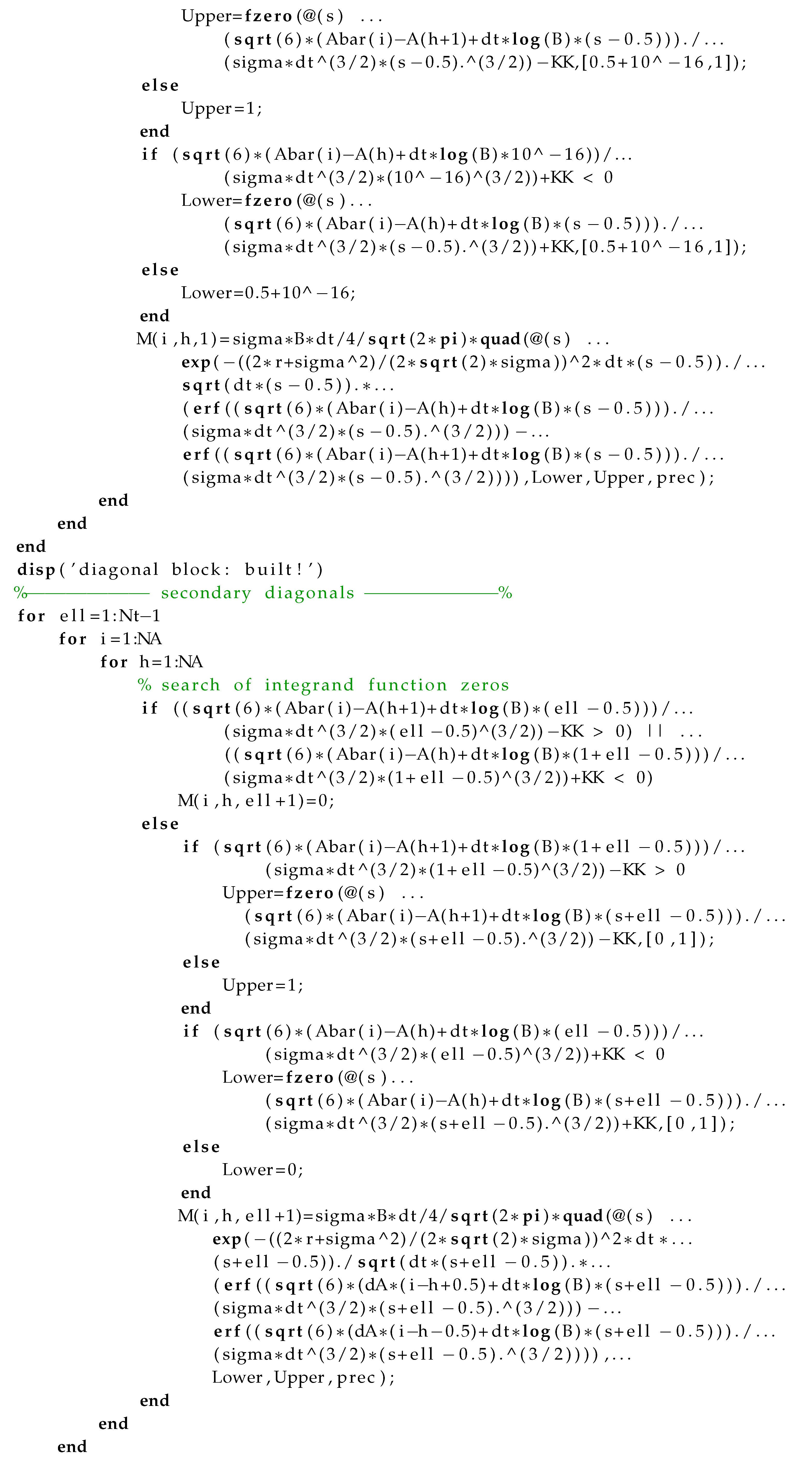
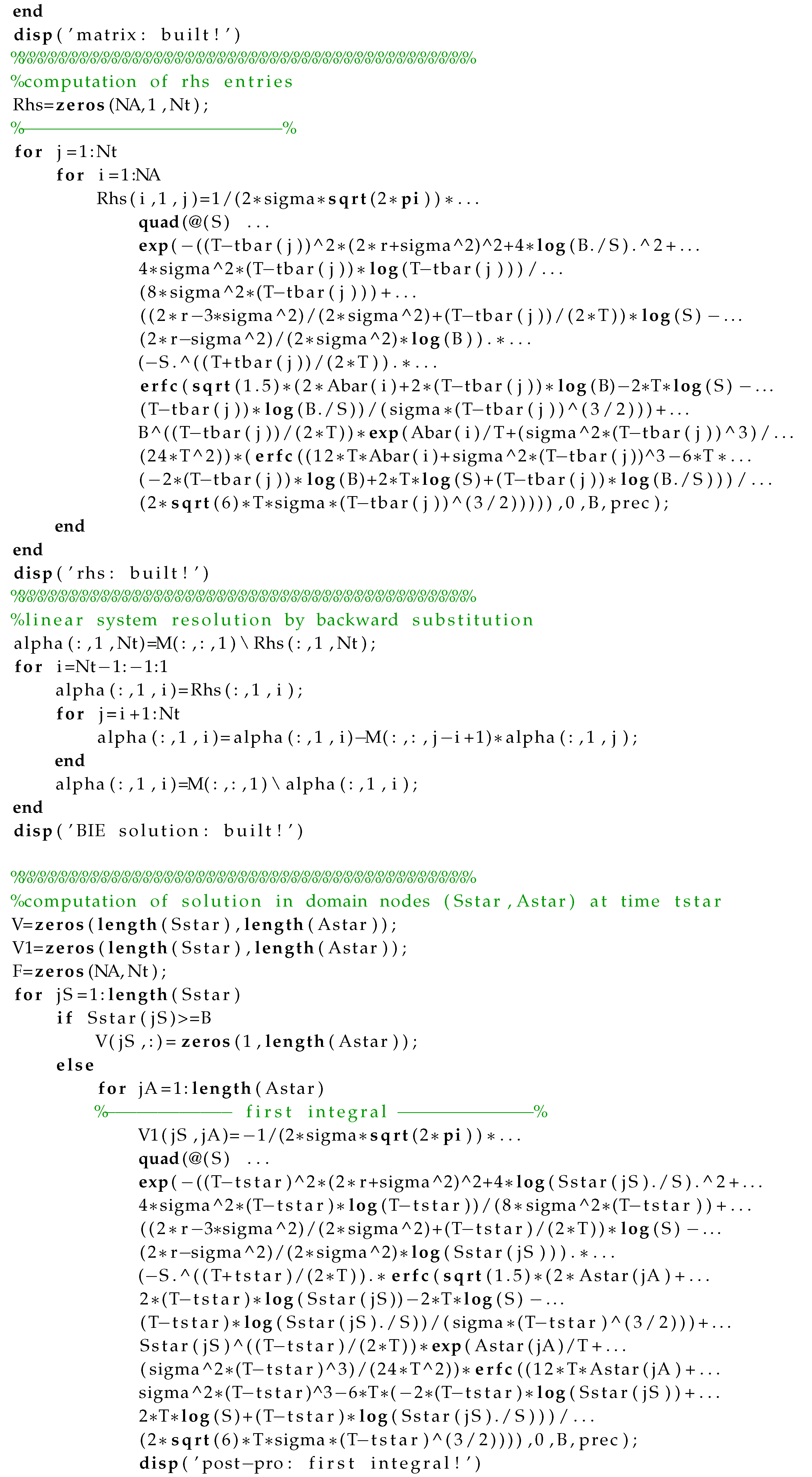
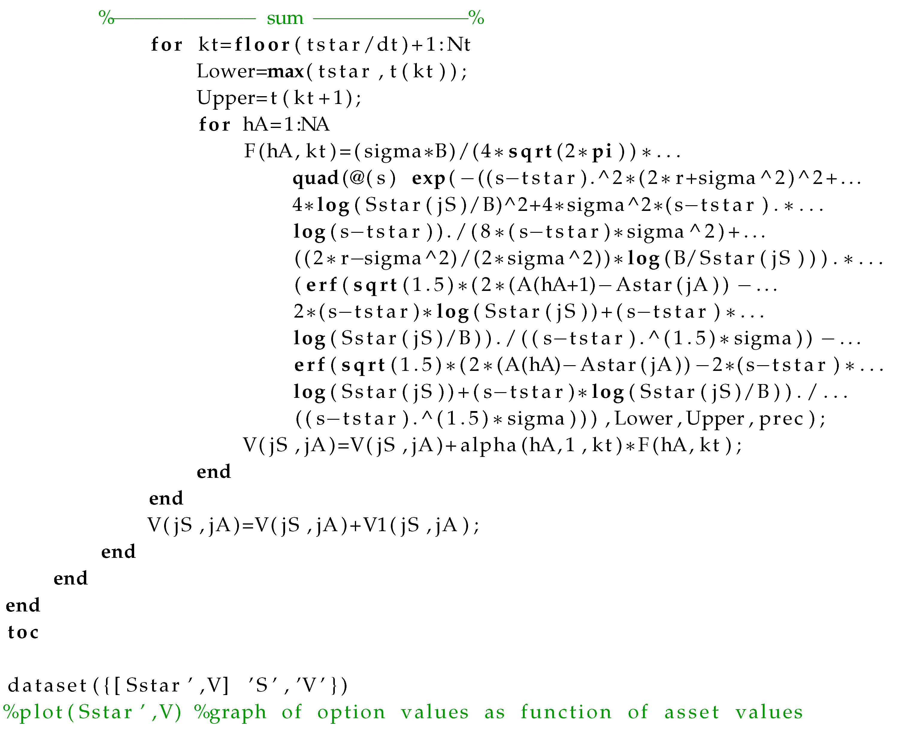
All the above-provided numerical results were obtained by codes developed with MATLAB^® Release 2007b running on a laptop computer (CPU Intel i5, 4 Gb RAM). The code implementing the SABO algorithm is given below.

References

- Hull, J. Options, Futures, and Other Derivatives, 8th ed.; Pearson-Prentice Hall: Upper Saddle River, NJ, USA, 2011. [Google Scholar]
- Boyle, P.; Potapchik, A. Prices and sensitivities of Asian options: A survey. Insur. Math. Econ. 2008, 42, 189–211. [Google Scholar] [CrossRef]
- Cao, G.; Wang, Y. Risk-neutral pricing for geometric average Asian options with floating strike. J. Chin. Acad. Sci. 2015, 32, 13–17. [Google Scholar]
- Aimi, A.; Guardasoni, C. Collocation Boundary Element Method for the pricing of Geometric Asian Options. Eng. Anal. Bound. Elem. 2017, 92, 90–100. [Google Scholar] [CrossRef]
- Aimi, A.; Diazzi, L.; Guardasoni, C. Numerical Pricing of Geometric Asian Options with Barriers. Math. Methods Appl. Sci. 2018, submitted. [Google Scholar]
- Guardasoni, C.; Sanfelici, S. A Boundary Element approach to barrier option pricing in Black-Scholes framework. Int. J. Comput. Math. 2016, 93, 696–722. [Google Scholar] [CrossRef]
- Guardasoni, C. Semi-Analytical method for the pricing of Barrier Options in case of time-dependent parameters (with Matlab codes). Commun. Appl. Ind. Math. 2018, 9, 42–67. [Google Scholar] [CrossRef]
- Ballestra, L.; Pacelli, G. A boundary element method to price time-dependent double barrier options. Appl. Math. Comput. 2011, 218, 4192–4210. [Google Scholar] [CrossRef]
- Wilmott, P. On Quantitative Finance; John Wiley and Sons: Hoboken, NJ, USA, 2000. [Google Scholar]
- Barucci, E.; Polidoro, S.; Vespri, V. Some results on partial differential equations and Asian options. Math. Model. Methods Appl. Sci. 2001, 11, 475–497. [Google Scholar] [CrossRef]
- Polidoro, S. Uniqueness and representation theorems for solutions of Kolmogorov-Fokker-Planck equations. Rendiconti di Matematica e delle sue Applicazioni 1995, 15, 535–560. [Google Scholar]
- Hörmander, L. Hypoelliptic second order differential equations. Acta Math. 1967, 119, 147–171. [Google Scholar] [CrossRef]
- Aimi, A.; Diligenti, M.; Guardasoni, C. Energetic BEM for the numerical solution of 2D hard scattering problems of damped waves by open arcs. Springer INdAM Series 2018, accepted. [Google Scholar]
- Hugger, J. A fixed strike Asian option and comments on its numerical solution. ANZIAM J. 2004, 45, C215–C231. [Google Scholar] [CrossRef]
- Hugger, J. Wellposedness of the boundary value formulation of a fixed strike Asian option. J. Comput. Appl. Math. 2006, 185, 460–481. [Google Scholar] [CrossRef]
- Kangro, R. Lecture Notes on Computational Finance; Technical Report; University of Tartu: Tartu, Estonia, 2011. [Google Scholar]
© 2018 by the authors. Licensee MDPI, Basel, Switzerland. This article is an open access article distributed under the terms and conditions of the Creative Commons Attribution (CC BY) license (http://creativecommons.org/licenses/by/4.0/).