Abstract
A dynamical model of Zika virus (ZIKV) epidemic with direct transmission, sexual transmission, and vertical transmission is developed. A sub-optimal control problem to counter against the disease is proposed including three controls: vector elimination, vector-to-human contact reduction, and sexual contact reduction. Each control variable is discretized into piece-wise constant intervals. The problem is solved by Differential Evolution (DE), which is one of the evolutionary algorithm developed for optimization. Two scenarios, namely four time horizons and eight time horizons, are compared and discussed. The simulations show that models with controls lead to decreasing the number of patients as well as epidemic period length. From the optimal solution, vector elimination is the prioritized strategy for disease control.
1. Introduction
Despite being discovered in Africa and named after a forest in Uganda in 1947, there are only several reported cases of Zika virus (ZIKV) infection before 2007. The virus itself is a mosquito-borne virus from the genus flavivirus that is transmitted primarily through the bite of Aedes mosquitoes. At first, the ZIKV infection was not considered a threat due to its mild symptoms such as rashes, headache, malaise, and fever [1]. Besides, the mortality rate of ZIKV infection is considered negligible, unlike other Flavivirus infections such as dengue and yellow fever. However, the announcement [2] on the possible association between the ZIKV infection and the increasing number of newborn babies with microcephaly in 2015 raised the alarm and public awareness of this outbreak. There is some correlative evidence reported from Brazil, Colombia, and other Latin America countries [3,4].
Some previous studies suggest that ZIKV could pass from pregnant mothers to their baby through the intrauterine infection, and microcephaly also happened during this process. Beside vector-mediated transmission and intrauterine (or vertical) transmission, ZIKV could also transmit through sexual transmission [5]. Apart from being detected in blood and semen [6], researchers found that the virus persists in semen and urine after it disappeared from the serum [7]. Moreover, it could pass on even before the patient develops the symptoms [8]. To control the outbreak, it can be seen that only relying on reducing the number of mosquito population or preventing the contact between host and vectors might be insufficient. The control strategy should include reducing the sexual transmission and vertical transmission as well.
A dynamical model was a popular tool for describing and analyzing various diseases. It was used to describe the mechanism functions and causes abnormality in some non-infectious diseases such as diabetes [9,10]. In prior publications [11,12,13], models with systems of ordinary differential equations were utilized for describing the behavior of infectious virus such as Zika. Optimal control is one of the popular methods for finding the solution that will minimize the objective function value. According to some publications [14,15], optimal control can be used to find the best strategy associated with the implemented cost and the provided situations. The optimal solutions for some flavivirus control such as chikungunya [16] and dengue [17] have been studied.
In this paper, we develop the ZIKV virus infection model using some previous works [12,13,18]. The model consists of three populations: adult humans, newborn babies human, and mosquitoes. Three controls are selected from the suggestions of the World Health Organization(WHO) [19] and health authorities [20]: using larvicide and adulticide to reduce the mosquito population, using insect repellents to prevent mosquito biting, and abstaining from sexual activity or using protection to prevent pregnancy.
Regarding optimal control and sub-optimal control problem, there are direct and indirect methods for solving the problems. The indirect approaches, such as Pontryagin’s Maximum Principle [21] and shooting method, are popular to find optimal solutions of some flavivirus control problems, for example, chikungunya [16] and dengue [17]. Previously, the authors also studied the optimal control problem of the Zika virus infection [18] by the indirect approach. However, the implementations for health authorities by these studies [16,17] are difficult to practically apply since the policies have to be varied continuously. Considering this drawback, we propose a sub-optimal control problem and find the solution that is both close to optimal and practical for real situation.
A sub-optimal control problem can be proposed through Model Predictive Control (MPC). MPC is the mathematical tool for controlling the optimization process in various fields such as industrial and medical technology [22]. It can be used from the simple to complex dynamic process, and the result control law is easy to implement. In our work, the control framework consists of a nonlinear system without constraints on spending cost or the final result of the system variables. This framework is related to the nonlinear unconstrained MPC schemes, which are those without terminal constraints and cost [23]. Furthermore, the study of Herty [24] estimated the suboptimality condition and suggested the guideline for the system containing a quadratic cost function.
In sub-optimal control problem, the previously continuous time horizon is discretized into N time horizons. Finding the solution of the controls in each time horizon helps archive the strategy which only applies the control at the constant level in each period. Caetano [25] and Yan [26] used the direct approach in finding the solutions to the sub-optimal disease control problem, and Yan [26] also used the Genetic Algorithm (GA).
Differential Evolution (DE) algorithm is an improved GA by Storn and Price [27]. DE algorithm is simple and fast, requires only a few control parameters and has high convergence attribute [28]. Thus, we find the solution of the sub-optimal control problem using the DE algorithm. The dynamical model is developed in Section 2 and the Differential Evolution is introduced in Section 3. The sub-optimal control problem is proposed through MPC and the numerical solutions are solved in Section 4. Lastly, the discussion and conclusion are presented in Section 5.
2. Dynamical Control Model for ZIKV Infection
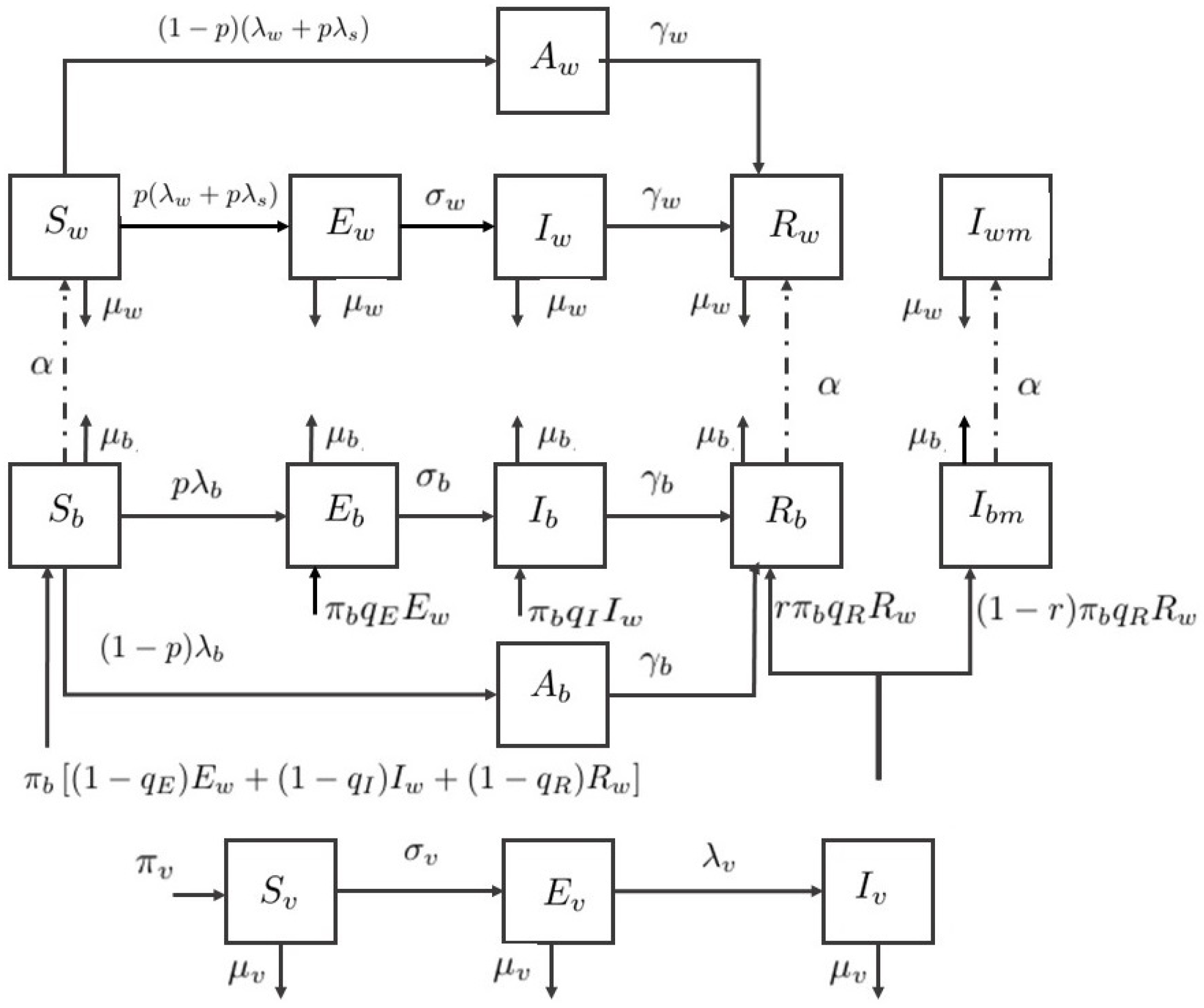
To describe the behavior of ZIKV infection, the dynamical compartment model with control is developed from the models of Gao et al. [12] and Agusto et al. [13]. The developed model consists of two human populations, adults and babies, and one mosquito (vector) population. The total newborn baby population consists of six classes: susceptible , exposed , asymptomatically infected , symptomatically infected without microcephaly, referred to as infected , infected with microcephaly , and recovered . The total adult population consists of six classes: susceptible , exposed , asymptomatically infected , symptomatically infected, referred to as infected , infected with microcephaly , and recovered . The total vector population consists of three classes: susceptible , exposed , and infected .
Hence, the total newborn baby population is , the total adult population is , the total vector population is , and the total human population is . The flow diagram of the compartment model is shown in Figure 1. Therefore, the ZIKV disease model with sexual transmission and vertical transmission is written by a system of differential equations under defined assumptions.
where
are the force of infection rates.

Figure 1.
Flow diagram of the Zika virus model.
In the system, a susceptible adult can be infected either through the bite of an infected vector or sexual contact with an exposed or symptomatically infected adult. The infected class is more contagious due to the higher load of viremia [29], hence the infection modification parameters are introduced for vector transmission and sexual transmission of an adult.
The newborn baby could be infected directly by mosquitoes or intrauterine via pregnant mother [30,31]. We assumed that the exposure rate of babies is different from adults, represented by the modification parameter . The infection modification is introduced as well. In the vertical transmission in babies, it occurred in some cases that newborn baby is infected during pregnancy [31,32].
We assumed that babies are born with infection due to vertical transmission by the parameter . Let the newborn birth rate be , the fraction of healthy newborn babies are , and the infected babies are the remaining , , and fractions. A recovered mother might give birth to the baby with microcephaly [30], and the baby born with microcephaly is assumed by the fraction in this paper.
Individuals with microcephaly experience a delay in development [33] and severe neurological disorders, so they are likely to have a short lifespan. Hence, we assumed that the adults with microcephaly do not reproduce or are involved in sexual transmission. The asymptomatically infected babies and adults are assumed to be noncontagious for both human and vector. Furthermore, the mortality rate from the disease is considered negligible. All parameter descriptions are summarized in Table 1.

Table 1.
Definition of variables and parameters.
Based on WHO [19] and Centers for Disease Control and Prevention (CDC) [20] suggestions, we considered vector, vertical, and sexual transmission the three control parameters selected for the model. The control variable is the use of mosquito repellents to prevent or reduce the biting from mosquitoes. The control variable is the procedure such as using protection for preventing pregnancy or unsafe sexual activity. The control variable is the use of insecticide to control or eliminate the mosquito population. By applying control strategy, forces of infection in the adult and baby populations decrease by the fraction of and . Correspondingly, the force of infection in vector population decreases by a fraction of . Lastly, the recruitment rate of mosquito decreases by a fraction of . It was also assumed that the mosquito death rate increases by , where . Remark: If the value of each control parameters , , and is equal to zero for all given period, the model in the system in Equation (1) would be the Zika virus model without controls.
The controls , , and are determined to minimize the given objective function:
subject to the state of system in Equation (1).
In Section 4, we find a set of controls that minimize the number of exposed humans, symptomatically infected humans, all mosquitoes and the costs related to the controlling implementation. Firstly, we introduce constants , , , , and as the weighted constants related to the exposed newborn babies, symptomatically infected newborn babies, exposed adults, symptomatically infected adults, and all mosquitoes, respectively. The constants , , and are the weighted constants of the control variables , , and , respectively. The terms , , and are the implementation costs of the three controls. The cost included in the first control might be the prices of using insect repellent, mosquito net, and herbal spray for instance. The cost included in the second control might be the prices of providing protections or warning leaflets about the safe sexual activity. The cost included in the last control could come from the expenses of using mosquito pesticides and the process implementation.
3. Differential Evolution
The differential evolution algorithm is a population-based optimization algorithm, introduced by Storn and Price [27,28]. It is also one of the Evolutionary algorithms developed to find the parameter values and optimize real parameters or functions. DE is suitable for various practical problems which are nonlinear, non-differentiable, and multi-dimensional. The process consists of four parts, namely initialization, mutation, crossover, and selection.
Suppose optimizing a problem consisting of D predicted parameters with number of population. Then, a -dimensional vector is solved by the following main steps until the best solution vector reaches the termination criteria.
Step 1. Initialization
The DE algorithm randomly selected a population of the parameter vectors where G is the generation number. Define the initial population as
that is each parameter , where is the lower bound and is the upper bound of the -th parameter and is a uniformly distributed random number between 0 and 1. Then, each of the parameter vectors will undergo mutation, crossover, and selection.
Step 2. Mutation
This process helps expand the search space. For each target vector , randomly select three vectors , , and such that each index i, , , and is different. Then, a mutant vector is generated by
where is the mutation vector and is called the donor vector.
Step 3. Crossover
Crossover or recombination process involves successful solutions from the previous generation. First, a trial vectors is produced from and by
where for a comparison to the crossover rate , and is a random index in that gets at least one component.
Step 4. Selection
The next generation vectors are selected by comparing the target vector and trial vector and selecting the one with the lowest objective function value. The objective function is given by comparing the value of , , , , and in the system in Equation (1) by applying vector and . Thus, the next generation vector is replaced by or under the following condition,
where J is the objective function (see Section 4).
Step 5. Repeating
After obtaining a new target vector, the mutation, crossover, and selection steps are repeated until the termination criteria are met.
4. Numerical Simulations for Sub-Optimal Control Problem
4.1. Sub-Optimal Control Problem
Given the objective function as defined in Equation (2), we assume there exists a solution of the optimal control problem characterized by the Pontryagins Maximum Principle [21]. Since the implemented result of the optimal control problem is complicated for the real situation, a sub-optimal control problem is proposed. The idea of sub-optimal control problem is based on the works of Rodrigues et. al. [16] and Moulay et al. [17], and the Model Predictive Control [22]. Regarding MPC, its strategy is based on the model of the system, a cost function which penalizes the undesirable behaviors, and constraints which represent the system limits. Furthermore, the stability and suboptimality of MPC can be estimated from the control horizon and the cost function [23,24]. For our nonlinear unconstrained model with a finite horizon, the continuous time horizon is discretized into N time horizon as
Then, each of the controls , , and , in each time horizon, is approximated by a piece-wise constant control such that
where , , and are constants and are referred to as the control parameters. Thus, for our model with now N control parameters for each , , and , we have total parameters to be minimized. Let
Then, the sub-optimal control problem is to
subject to the system in Equation (1) and J is as defined in Equation (2).
4.2. Numerical Simulations
The simulations in this work are constructed using the parameter values in Table 2. Since the Zika virus is still under investigation and discovery, some parameter values are obtained from the previous study of other mosquito-borne viruses. The initial conditions are also selected for the theoretical sense and illustration purpose. The initial conditions for the system in Equation (1) are given by , , , , , , 200,000, , , , , , 10,000, , and . The weight constants are given as , , , , , , , and . The total time span is 120 days, which is approximately four months.

Table 2.
Parameter values.
From [24], the performance bound, which depends on the time horizon N and the cost function, could be computed to estimate the distance between MPC cost and the optimal cost. It also suggests that the time horizon N should not be too small. Hence, in our simulation with the total time of 120 days, we consider two scenarios with the different time horizon N as follows: (i) with ; and (ii) with . All controls must be non-negative and let the maximum value be 0.9 since it is almost impossible to fully implement each control strategy. The numerical simulation from each scenario is generated with the DE algorithm with the maximum iteration of 150, , and . Number of population is 120 and 240 for Scenarios and , respectively.
(i) Scenario
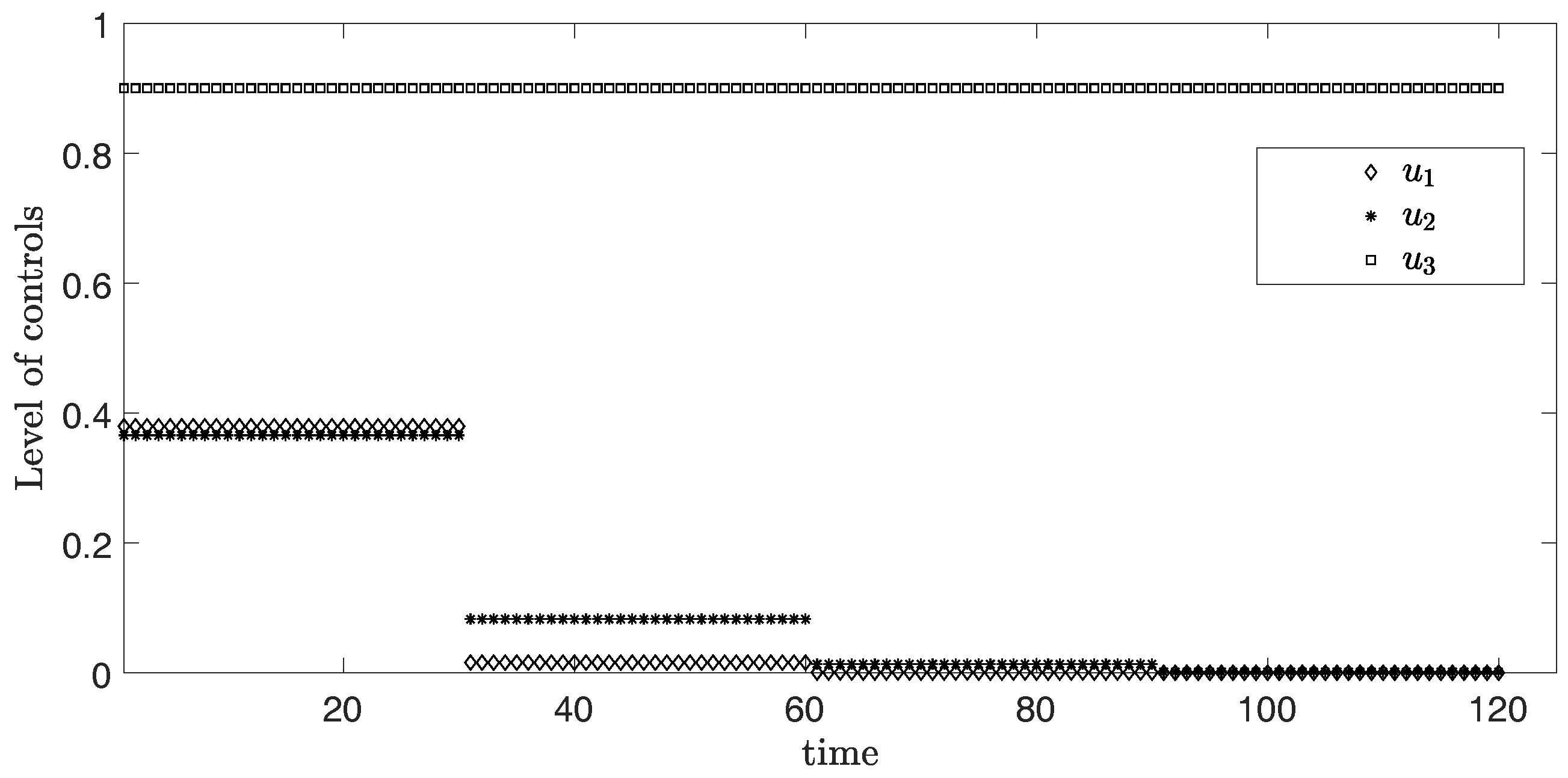
In this scenario, the period is 30 days or one month for each time horizon. Figure 2 represents the simulation of three controls over 120 days. From the graph, the levels of and are at the highest around 0.36 and 0.37 in the first month, respectively. After that, the levels of both controls and discretely drop in the second month and become approximately zero in the third month. Differently, the level of control stays at the maximum value 0.9 during the entire time.

Figure 2.
Level of controls from Scenario (i) .
The objective function value is , where the control values are:
(ii) Scenario
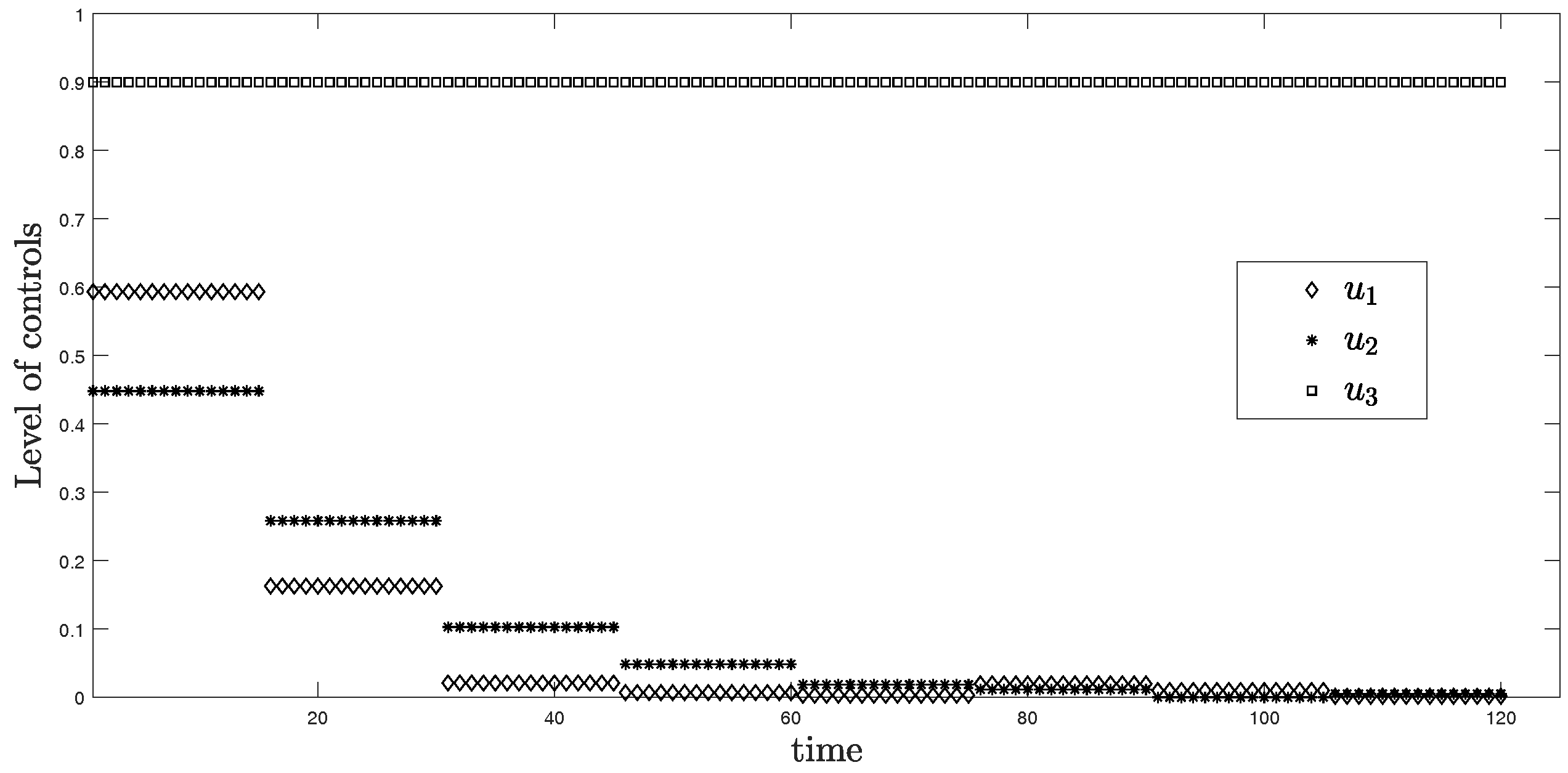
In this scenario, the period is 15 days or approximately two weeks for each time horizon. Figure 3 represents the simulation of three controls over 120 days. From the graph, is at the highest level around 0.6 in the first two weeks and discretely drops to approximately zero within one month. For , it reaches around 0.45 for the first two weeks, then drops to nearly zero after the second month. Differently, the level of control stays at the maximum value 0.9 during the entire time.
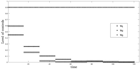
Figure 3.
Level of controls from Scenario (ii) .
The objective function value is , where the control values are:
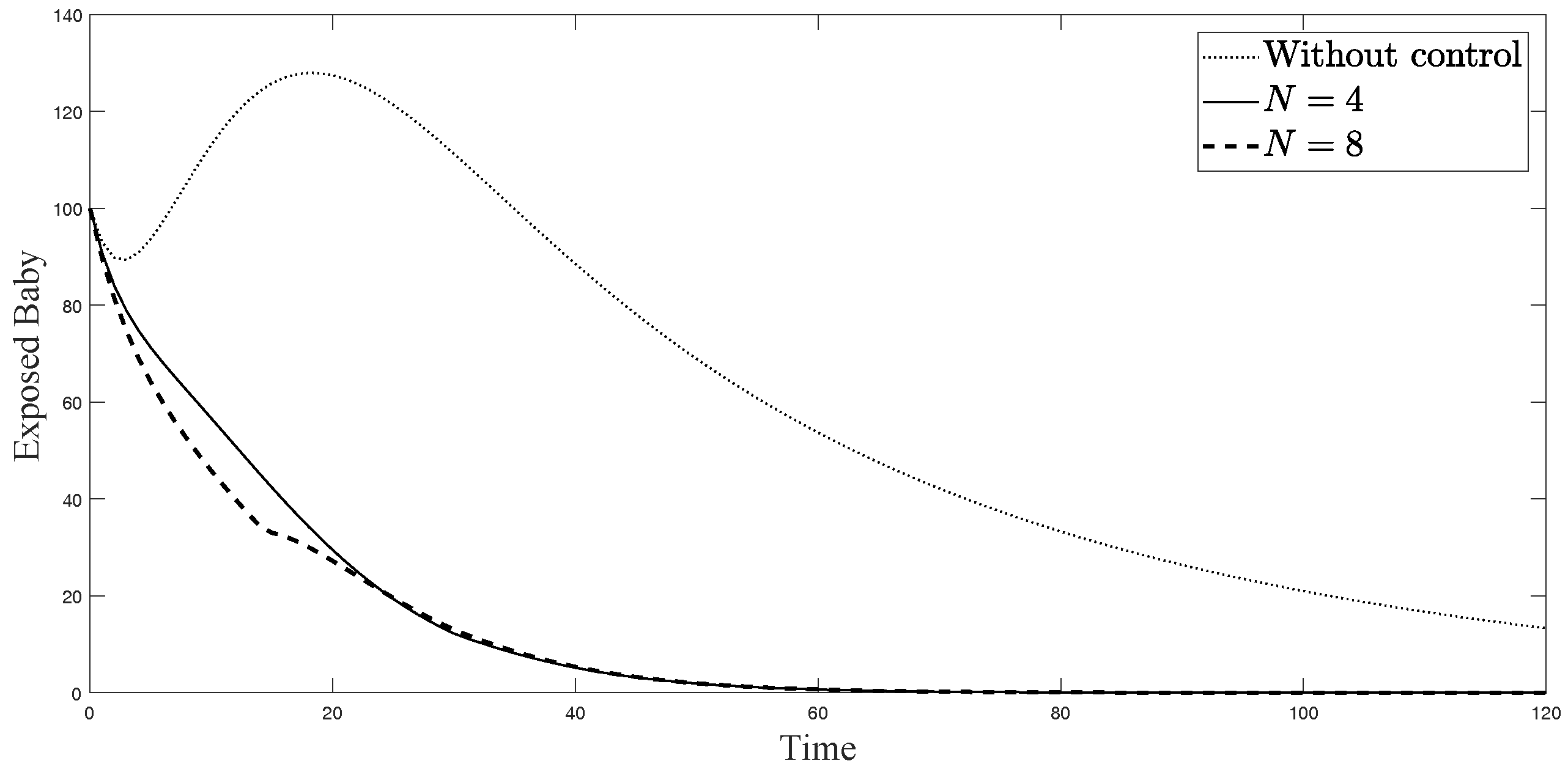
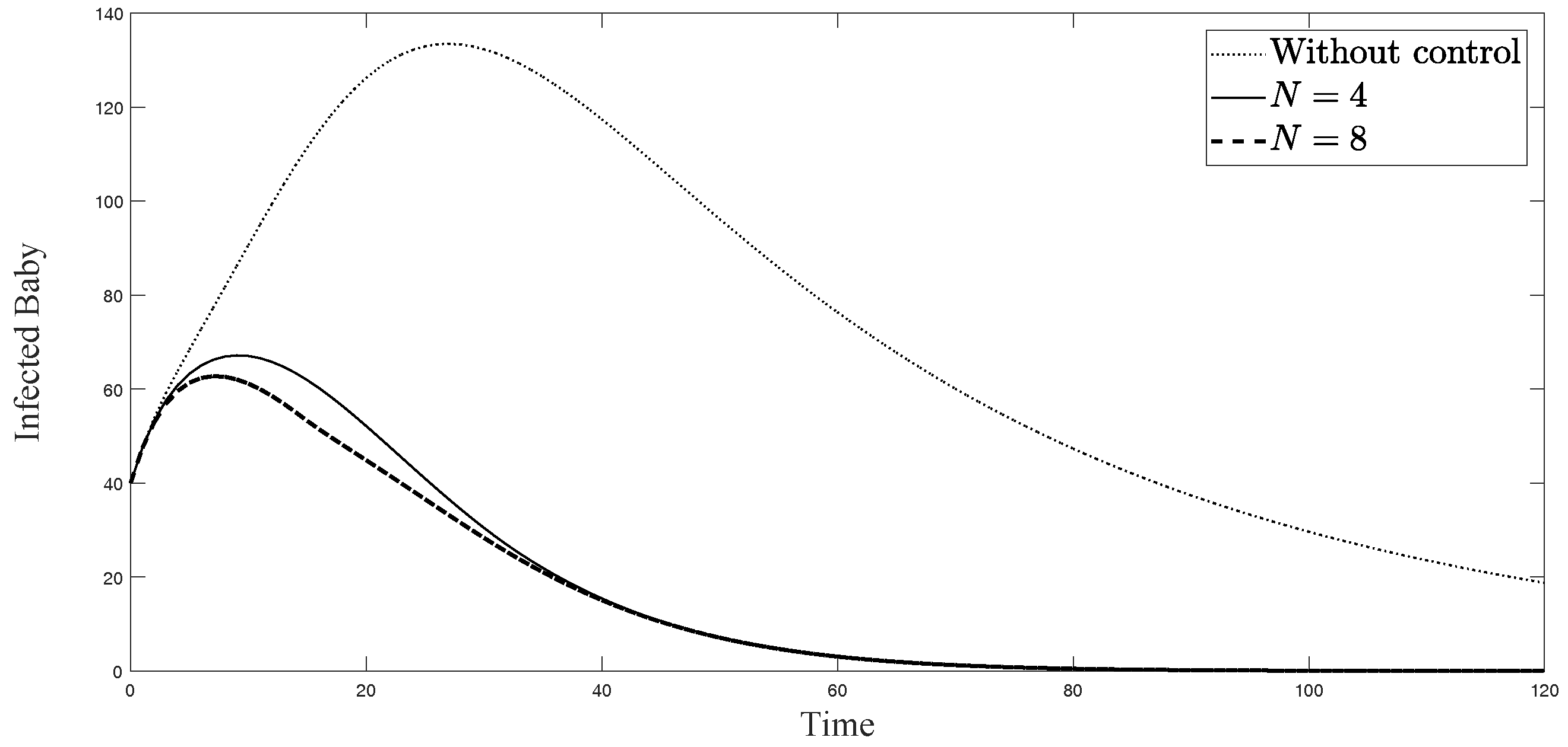
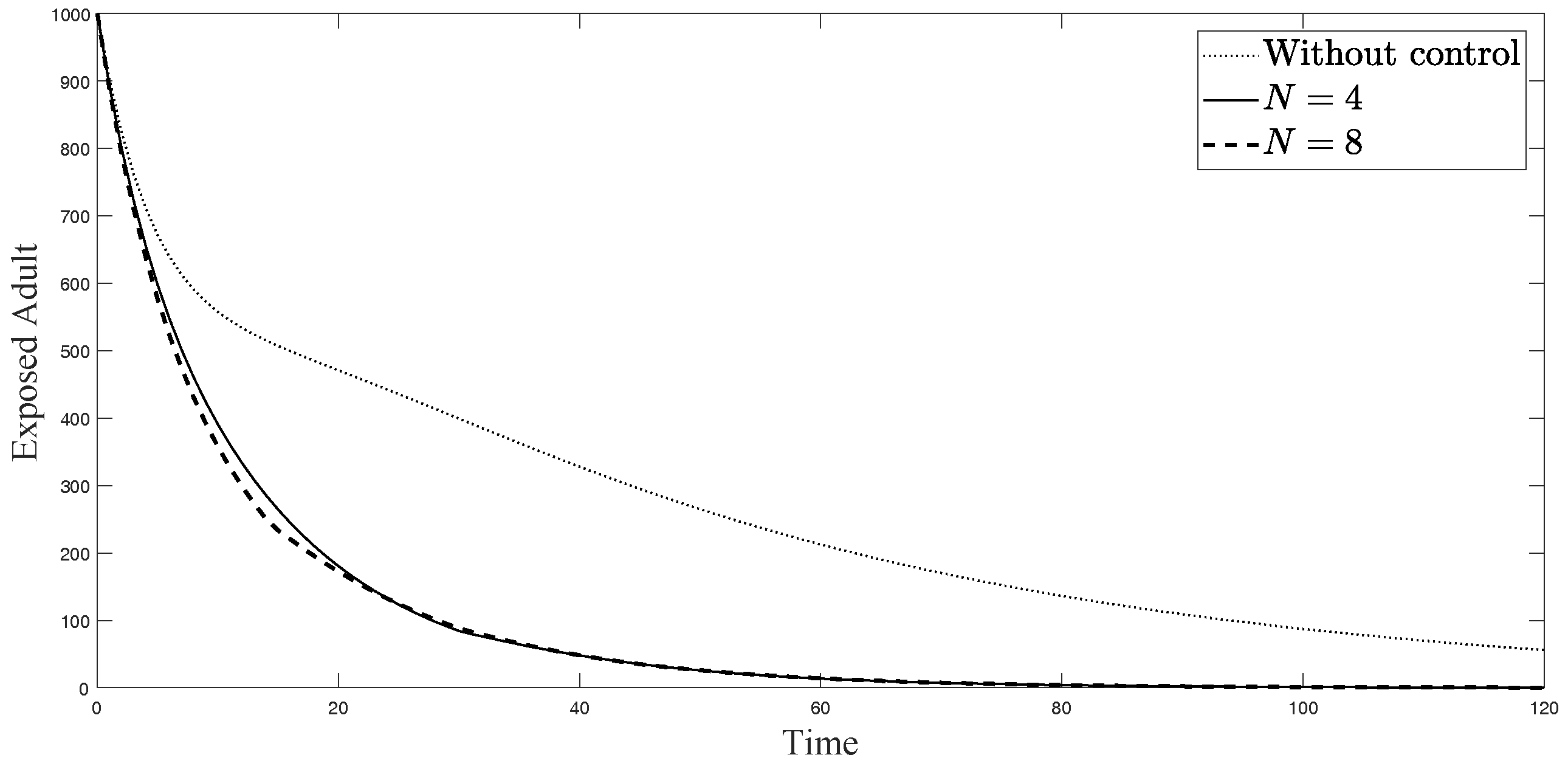
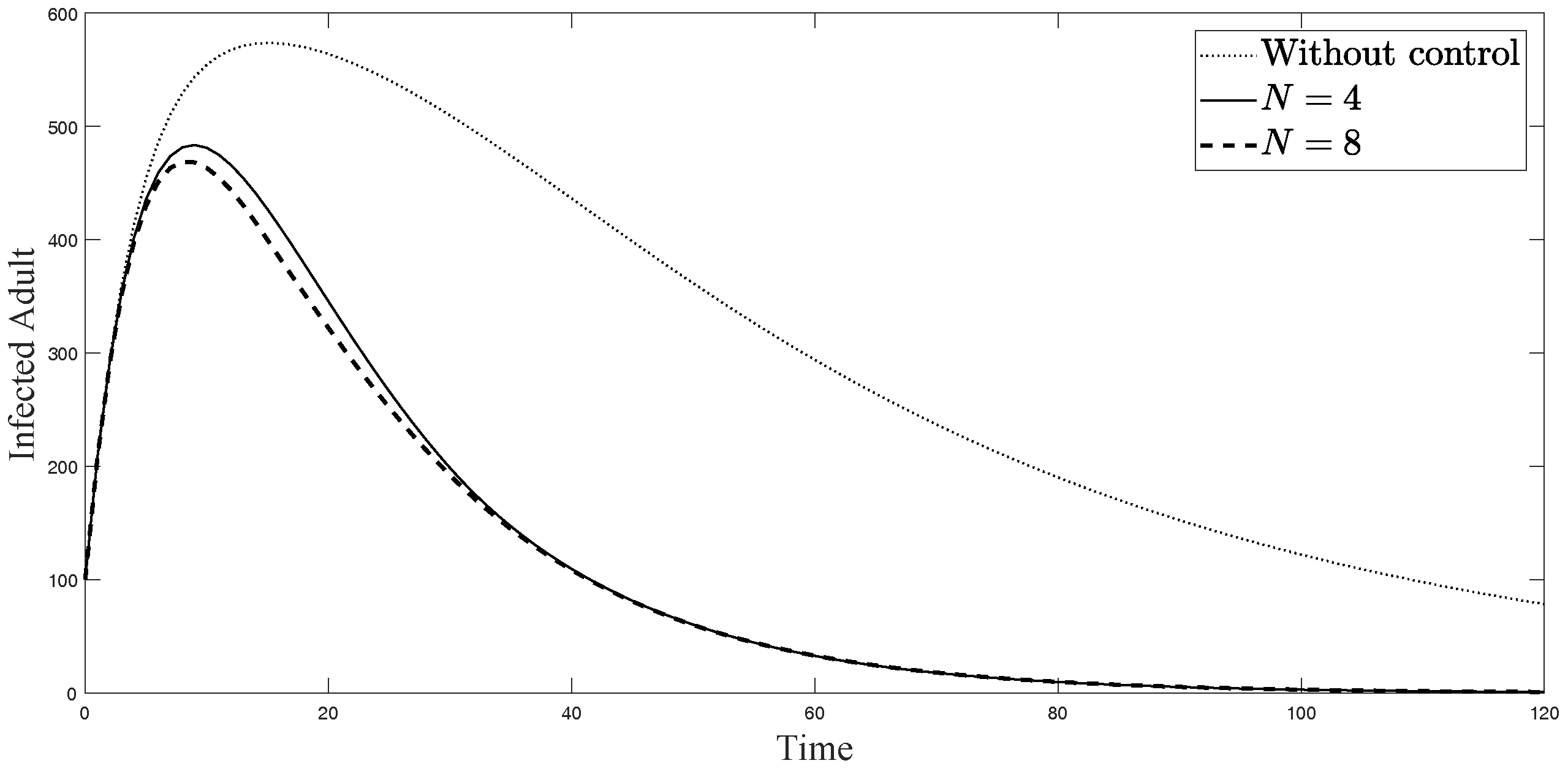
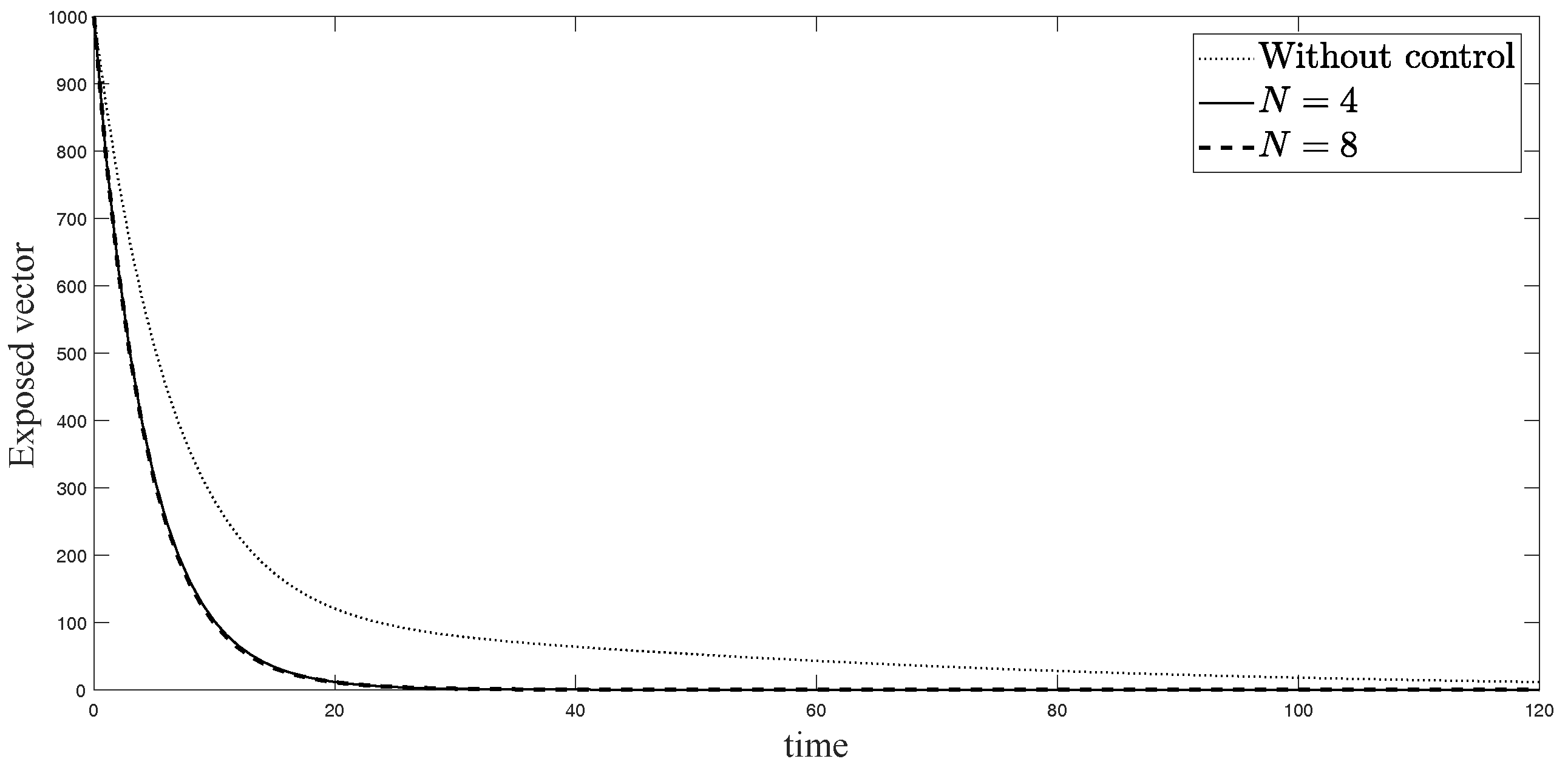
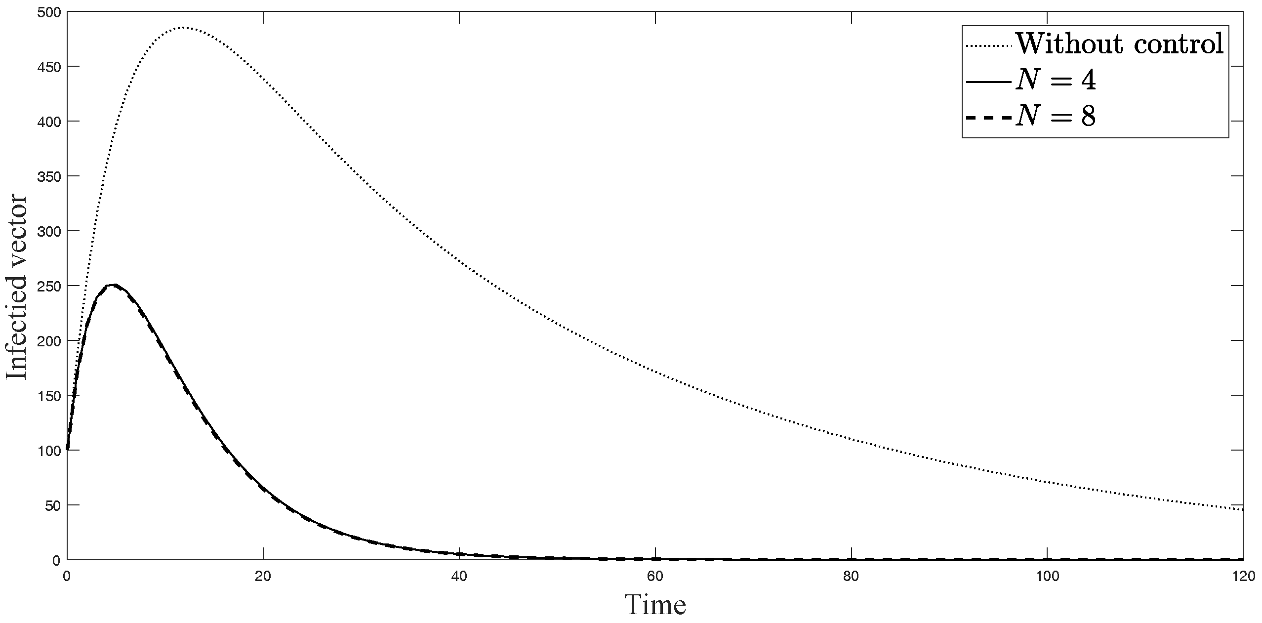
The simulations in Figure 4, Figure 5, Figure 6, Figure 7, Figure 8 and Figure 9 represent the number of exposed babies, infected babies, exposed adults, infected adults, exposed vectors and infected vectors, respectively. In each graph, the dotted line represents the model without control, the solid line represents the control model with Scenario , and the dashed line represents the control model with Scenario . In Figure 4, Figure 5, Figure 6, Figure 7, Figure 8 and Figure 9, the numbers of exposed and infected individuals from the model with controls are less than those of the model without control. This implies that control strategy ceases the serve of the disease. The models from both scenarios yield very close results where is slightly better. Notice in Figure 4, Figure 5, Figure 6 and Figure 7 that the disease spreads heavily during the first month. Later, those patients decrease and become stable after two months, corresponding to the drop in control and after two months. Thus, both and contribute to the control of the disease. The control contributes the most and becomes the top priority in the strategy.

Figure 4.
Simulation results of exposed newborn babies from: (i) the model without controls; (ii) the control model with ; and (iii) the control model with .

Figure 5.
Simulation results of symptomatically infected newborn babies from: (i) the model without controls; (ii) the control model with ; and (iii) the control model with .

Figure 6.
Simulation results of exposed adults from: (i) the model without controls; (ii) the control model with ; and (iii) the control model with .
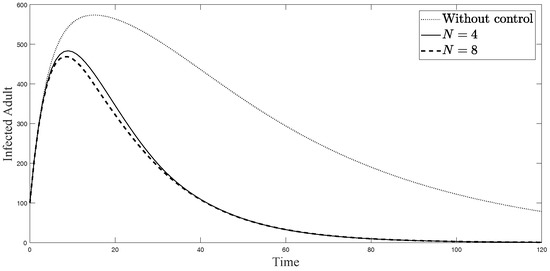
Figure 7.
Simulation results of symptomatically infected adults from: (i) the model without controls; (ii) the control model with ; and (iii) the control model with .
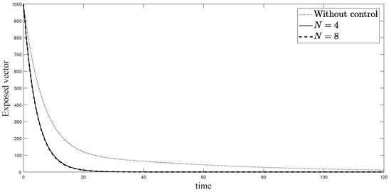
Figure 8.
Simulation results of exposed vectors: (i) the model without controls; (ii) the control model with ; and (iii) the control model with .
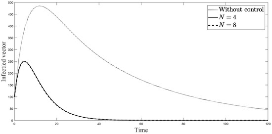
Figure 9.
Simulation results of infected vectors from: (i) the model without controls; (ii) the control model with ; and (iii) the control model with .
5. Conclusions
In this work, we developed the dynamical model of ZIKV disease with sexual transmission and vertical transmission. We proposed sub-optimal control problem with three control parameters: vector elimination, human–vector reduction, and human–human contact reduction. To find the control solution which is easy to implement, we partitioned the controls into discrete intervals. By using Differential Evolution, we solved and presented the numerical scenarios with four time horizons and eight time horizons. The simulations of both controls efficiently reduce the number of exposed and infected patients where the model with eight intervals yields a slightly better result. Controls , using repellents to prevent mosquito biting, and , avoiding pregnancy and unsafe sexual activity, should be applied mostly during the peak of the disease. After the disease dies out or becomes stable, the level of both controls will decrease. Mosquito elimination should be the first focus in controlling the disease, corresponding to the primary procedure announced by general health authorities. However, the cost associated with each control in this simulation is set to be equal. The consideration of adjusting the relative cost according to alternative scenarios might provide different results. Additionally, if more information is available in the future, the simulations should be conducted again using more precise data.
Author Contributions
Conceptualization, W.S.; Investigation, N.C. and W.S.; Methodology, W.S.; Visualization, N.C.; Writing—original draft, N.C.; and Writing—review and editing, W.S.
Funding
This research received no external funding.
Acknowledgments
This research was supported by Centre of Excellence in Mathematics, PERDO, CHE, Thailand and Golden Jubilee Scholarship from Faculty of science, Mahidol university, Thailand.
Conflicts of Interest
The authors declare no conflict of interest.
Abbreviations
The following abbreviations are used in this manuscript:
| WHO | World Health Organization |
| GA | Genetic Algorithm |
| DE | Differential Evolution |
References
- Dasti, J.I. Zika virus infections: An overview of current scenario. Asian Pac. J. Trop. Med. 2016, 7, 621–625. [Google Scholar] [CrossRef] [PubMed]
- European Centre for Disease Prevention and Control. Zika Virus Epidemic in the Americas: Potential Association with Microcephaly and Guillain-Barre Syndrome. Available online: https://ecdc.europa.eu/sites/portal/files/media/en/publications/Publications/zika-virus-americas-association-with-microcephaly-rapid-risk-assessment.pdf (accessed on 12 February 2017).
- World Health Organization. Microcephaly-Brazil: Disease Outbreak News. Available online: http://www.who.int/csr/don/archive/disease/microcephaly/en/ (accessed on 12 February 2017).
- World Health Organization. Zika Situation Report. Available online: http://www.who.int/emergencies/zika-virus/situation-report/12-february-2016/en/ (accessed on 12 February 2017).
- Coelho, F.C.; Durovni, B.; Saraceni, V.; Lemos, C.; Codeco, C.T.; Camargo, S.; de Carvalho, L.M.; Bastos, L.; Arduini, D.; Villela, D.A.; et al. Higher incidence of Zika in adult women than adult men in Rio de Janeiro suggests a significant contribution of sexual transmission from men to women. Int. J. Infect. Dis. 2016, 51, 128–132. [Google Scholar] [CrossRef] [PubMed]
- Atkinson, B.; Hearn, P.; Afrough, B.; Lumley, S.; Carter, D.; Aarons, E.J.; Simpson, A.J.; Brooks, T.J.; Hewson, R. Detection of Zika virus in semen. Emerg. Infect. Dis. 2016, 22, 940. [Google Scholar] [CrossRef] [PubMed]
- Musso, D.; Roche, C.; Robin, E.; Nhan, T.; Teissier, A.; Cao-Lormeau, V.-M. Potential sexual transmission of Zika virus. Emerg. Infect. Dis. 2015, 21, 359–361. [Google Scholar] [CrossRef] [PubMed]
- Foy, B.D.; Kobylinski, K.C.; Foy, J.L.; Blitvich, B.J.; da Rosa, A.T.; Haddow, A.D.; Lanciotti, R.S.; Tesh, R.B. Probable non-vector-borne transmission of Zika virus. Emerg. Infect. Dis. 2011, 17, 880–882. [Google Scholar] [CrossRef] [PubMed]
- Chalishajar, D. Mathematical Analysis of Insulin-glucose feedback system of Diabetes. J. Eng. Appl. Sci. 2014, 5, 36–58. [Google Scholar]
- Chalishajar, D.; Geary, D.; Cox, G. Review Study of Detection of Diabetes Models through Delay Differential Equations. Appl. Math. 2016, 7, 1087–1102. [Google Scholar] [CrossRef]
- Kucharski, A.J.; Funk, S.; Eggo, R.M.; Mallet, H.-P.; Edmunds, W.J.; Nilles, E.J. Transmission dynamics of Zika virus in island populations: A modelling analysis of the 2013-14 French Polynesia outbreak. PLoS Negl. Trop. Dis. 2016, 10, 0004726. [Google Scholar] [CrossRef] [PubMed]
- Gao, D.; Lou, Y.; He, D.; Porco, T.C.; Kuang, Y.; Chowell, G.; Ruan, S. Prevention and control of Zika as a mosquito-borne and sexually transmitted disease: a mathematical modeling analysis. Sci. Rep. 2016, 6, 28070. [Google Scholar] [CrossRef] [PubMed]
- Agusto, F.B.; Bewick, S.; Fagan, W.F. Mathematical model of Zika virus with vertical transmission. Infect. Dis. Model. 2017, 2, 244–267. [Google Scholar] [CrossRef] [PubMed]
- Lashari, A.A.; Zaman, G. Optimal control of a vector borne disease with horizontal transmission. Nonlinear Anal. 2012, 13, 203–212. [Google Scholar] [CrossRef]
- Yan, X.; Zou, Y.; Li, J. Optimal quarantine and isolation strategies in epidemics control. World J. Model. Simul. 2007, 3, 202–211. [Google Scholar]
- Rodrigues, H.S.; Monteiro, M.T.T.; Torres, D.F. Vaccination models and optimal control strategies to dengue. Math. Biosci. 2014, 247, 1–12. [Google Scholar] [CrossRef] [PubMed]
- Moulay, D.; Aziz-Alaoui, M.; Kwon, H.-D. Optimal control of chikungunya disease: Larvae reduction, treatment and prevention. Math. Biosci. Eng. 2012, 9, 369–392. [Google Scholar] [CrossRef] [PubMed]
- Chaikham, N.; Sawangtong, W. Optimal control of Zika virus infection by vector elimination, vector-to-human and human-to-human contact reduction. Adv. Differ. Equ. 2017, 2017, 177. [Google Scholar] [CrossRef]
- World Health Organization. Mosquito Control: Can It Stop Zika at Source? Available online: http://www.who.int/emergencies/zika-virus/articles/mosquito-control/en/ (accessed on 12 February 2017).
- Centers for Disease Control and Prevention (CDC), Update: Interim Guidelines for Prevention of Sexual Transmission of Zika Virus-United States. 2016. Available online: https://emergency.cdc.gov/han/han00388.asp (accessed on 5 July 2017).
- Lenhart, S.; Workman, J.T. Basic Optimal Control Problems. In Optimal Control Applied to Biological Models; CRC Press: Boca Raton, FL, USA, 2007; pp. 1–18. [Google Scholar]
- Camacho, E.F.; Alba, C.B. Introduction to Model Predictive Control. In Model Predictive Control; Springer Science & Business Media: Berlin/Heidelberg, Germany, 2007; pp. 1–30. [Google Scholar]
- Grüne, L. Analysis and design of unconstrained nonlinear MPC schemes for finite and infinite dimensional systems. SIAM J. Control Optim. 2009, 48, 1206–1228. [Google Scholar] [CrossRef]
- Herty, M.; Zanella, M. Performance bounds for the mean-field limit of constrained dynamics. arXiv, 2015; arXiv:1511.08364. [Google Scholar]
- Caetano, M.A.L.; Yoneyama, T. Optimal and sub-optimal control in Dengue epidemics. Optim. Control Appl. Methods 2011, 22, 63–73. [Google Scholar] [CrossRef]
- Yan, X.; Zou, Y. Optimal and sub-optimal quarantine and isolation control in SARS epidemics. Math. Comput. Model. 2008, 47, 235–245. [Google Scholar] [CrossRef]
- Price, K.; Storn, R.; Lampinen, J. The Differential Evolution Algorithm. In Differential Evolution: A Practical Approach to Global Optimization; Springer: New York, NY, USA, 2005; pp. 37–134. ISBN 978-3-540-31306-9. [Google Scholar]
- Storn, R.; Price, K. Differential evolution—A simple and efficient heuristic for global optimization over continuous spaces. J. Glob. Optim. 1997, 11, 341–359. [Google Scholar] [CrossRef]
- Hills, S.L. Transmission of Zika virus through sexual contact with travelers to areas of ongoing transmission-continental United States, 2016. Morb. Mortal. Wkly. Rep. 2016, 65, 215–216. [Google Scholar] [CrossRef] [PubMed]
- Moore, C.A.; Staples, J.E.; Dobyns, W.B.; Pessoa, A.; Ventura, C.V.; Fonseca, E.B.D.; Ribeiro, E.M.; Ventura, L.O.; Neto, N.N.; Arena, J.E.; et al. Characterizing the Pattern of Anomalies in Congenital Zika Syndrome for Pediatric Clinicians. JAMA Pediatr. 2017, 171, 288–295. [Google Scholar] [CrossRef] [PubMed]
- Schuler-Faccini, L.; Ribeiro, E.M.; Feitosa, I.M.; Horovitz, D.D.; Cavalcanti, D.P.; Pessoa, A.; Doriqui, M.J.; Neri, J.I.; Neto, J.M.; Wanderley, H.Y.; et al. Possible Association Between Zika Virus Infection and Microcephaly—Brazil, 2015. Morb. Mortal. Wkly. Rep. 2016, 65, 59–62. [Google Scholar] [CrossRef] [PubMed]
- Besnard, M.; Lastere, S.; Teissier, A.; Cao-Lormeau, V.M.; Musso, D. Evidence of perinatal transmission of Zika virus, French Polynesia, December 2013 and February 2014. Euro Surveill. 2014, 19, 20751. [Google Scholar] [CrossRef] [PubMed]
- Carter, M.T.; Mirzaa, G.; McDonell, L.M.; Boycott, K.M. Microcephaly-Capillary Malformation Syndrome. 2013 December 12. GeneReviews®, Seattle (WA): University of Washington, Seattle, 1993–2018. Available online: https://www.ncbi.nlm.nih.gov/books/NBK174452/ (accessed on 5 July 2017).
- Wikipedia. List of Sovereign States and Dependent Territories by Birth Rate. Available online: https://en.wikipedia.org/wiki/List_of_sovereign_states_and_dependencies_by_total_fertility_rate (accessed on 1 February 2017).
- Manore, C.; Hickmann, J.; Xu, S.; Wearing, H.; Hyman, J. Comparing dengue and chikungunya emergence and endemic transmission in a. aegypti and a. albopictus. J. Theor. Biol. 2014, 356, 174–191. [Google Scholar] [CrossRef] [PubMed]
- Bewick, S.; Fagan, W.; Calabrese, J.; Agusto, F. Zika virus: Endemic versus epidemic dynamics and implications for disease spread in the Americas. bioRxiv 2016. [Google Scholar] [CrossRef]
- Andraud, M.; Hens, N.; Marais, C.; Beutels, P. Dynamic epidemiological models for dengue transmission: A systematic review of structural approaches. PLoS ONE 2012, 7, 49085. [Google Scholar] [CrossRef] [PubMed]
- Trpis, M.; Haussermann, W. Dispersal and other population parameters of aedes aegypti in an african village and their possible significance in epidemiology of vector-borne diseases. Am. J. Trop. Med. Hyg. 1986, 35, 1263–1279. [Google Scholar] [CrossRef] [PubMed]
© 2018 by the authors. Licensee MDPI, Basel, Switzerland. This article is an open access article distributed under the terms and conditions of the Creative Commons Attribution (CC BY) license (http://creativecommons.org/licenses/by/4.0/).

