Abstract
In this paper, we examine the finite mixture (FM) model with a flexible class of two-piece distributions based on the scale mixtures of normal (TP-SMN) family components. This family allows the development of a robust estimation of FM models. The TP-SMN is a rich class of distributions that covers symmetric/asymmetric and light/heavy tailed distributions. It represents an alternative family to the well-known scale mixtures of the skew normal (SMSN) family studied by Branco and Dey (2001). Also, the TP-SMN covers the SMN (normal, t, slash, and contaminated normal distributions) as the symmetric members and two-piece versions of them as asymmetric members. A key feature of this study is using a suitable hierarchical representation of the family to obtain maximum likelihood estimates of model parameters via an EM-type algorithm. The performances of the proposed robust model are demonstrated using simulated and real data, and then compared to other finite mixture of SMSN models.
1. Introduction
Finite mixture models are highly demanded in machine-learning analysis, due to their properties, computational tractability, and for being a good approximation for continuous densities [1]. They are also an important statistical tool for many applications in clustering, discriminant analysis, image processing and satellite imaging [2]. Beyond the already known results provided for the finite mixture of normal distributions (FM-NOR) model in the literature [1], recent developments cover symmetric/asymmetric and light/heavy tailed distributions. One of these is the novel class of finite mixture of multivariate skew-normal mixture (FM-SN) models [3,4], which provides some advantages over the normal mixtures: the normal components allow an arbitrarily close modeling of any distribution by increasing the number of components, and, in the context of supervised learning, groups of observations represented by asymmetrically distributed data can lead to the wrong classification. The components of skew-normal mixture models, however, capture skewness due to their flexibility [1]. In addition, a robust extension of the FM-SN model to robust finite mixture of skew-t (FM-ST) has been done in the influential works of [3,5,6,7]. The FM-ST components, too, capture both skewness and extreme observations due to their flexibility [8].
The SMSN family is a rich and very strong flexible class of distributions which covers the light/heavy-tailed distributions; e.g., skew-normal (SN), skew-t (ST), skew-slash (SSL) and skew contaminated-normal (SCN) distributions, and has been widely considered in many statistical models, especially FM models (see e.g., [5,9,10,11,12,13,14,15]). The SMSN family is an extension of the skewed version of the well-known symmetric scale mixtures of the normal (SMN) family which contains the light/heavy-tailed members: the normal (N), t (T), slash (SL) and contaminated-normal (CN) distributions [16]. Lange et al. [17], Lange and Sinsheimer [18], and Maleki and Nematollahi [19] used the SMN family in an application of robust statistical modeling. A two-piece distribution based on the symmetrical distributions with various scales is an alternative approach to model atypical data (see e.g., [10,20,21,22,23,24]). In our approach, we have used the two-piece distributions based on the SMN family. This family, called the two-piece distributions based on the scale mixtures of normal (TP-SMN), and analogy of the SMSN family, contains the light/heavy-tailed members: the two-piece normal (TP-N), two-piece t (TP-T), two-piece slash (TP-SL) and two-piece contaminated-normal (TP-CN) distributions as its members.
In this paper, we consider the TP-SMN family of distributions as a two-component mixture of truncated SMN distributions on a special two partition of the real domain (), and then propose the finite mixture of this family, called FM-TP-SMN models. It represents an alternative family to the well-known scale mixtures of skew normal (SMSN) family studied by [25]. We have also used a hierarchical representation of the FM-TP-SMN and implemented an expectation-maximization (EM)-type algorithm for finding the maximum likelihood (ML) estimates of the proposed model. Studies by [21,23], show that by truncating the distribution in two partitions, makes it possible to obtain a better fit of empirical distribution because, the subjacent process of the complete likelihood is modeled. This way, the “two-piece” modeling is a direct competitor against the FM-SMSN family of distributions [21].
The rest of this paper is organized as follows. In Section 2, we review some main properties of the TP-SMN family and represent this family as a two-component mixture of the truncated SMN distributions. In Section 3, the FM-TP-SMN model is introduced and the ML estimates of the proposed model parameters via an EM-type algorithm are provided. In Section 4, numerical studies with an application of the proposed models and estimates are considered. Some conclusions and ideas for future research are offered in Section 5.
2. The Two-Piece Scale Mixtures of Normal Distributions
In this section, we analyze some necessary properties of the TP-SMN family of distributions for our proposed FM model.
The well-known SMN family introduced by [16] (the basis of the robust asymmetric TP-SMN family), has the following probability density function (PDF) and stochastic representation. Let , then its PDF is
and its stochastic representation is
where represents the density of distribution, is the cumulative distribution function (CDF) of the scale mixing random variable U, which can be indexed by a scalar or vector of parameters , and W is a standard normal random variable that is independent of U.
The TP-SMN is a rich family of distributions that covers the asymmetric light-tailed TP-N (also called the epsilon-skew-normal; [26]), the asymmetric heavy-tailed TP-T, TP-SL and TP-CN distributions, and their corresponding symmetric members. Note that symmetric members of the TP-SMN and SMSN classes are the SMN family. In terms of density, for this family can be represented as
where is the slant parameter, is given by (1) and is denoted by with and , for which , , , and U is the scale mixing random variable in (2).
Different TP-SMN member distributions in (3) are obtained by several distributions for scale mixing random variable U in (2), as follows:
- Two-piece normal (TP-N): with probability one,
- Two-piece t (TP-T): , i.e., ,
- Two-piece slash (TP-SL): , i.e., ,
- Two-piece contaminated normal (TP-CN): , i.e., .
For more details and statistical properties of the TP-SMN family, see [20,23].
Further, the two-piece distributions can be represented as the two-component mixture with separated supports, i.e., left and right half basic distributions [20] (Equation (4)), especially when with PDF given in (3), two-component mixture left and right half SMN distributions with special component probabilities as follows:
Note in Equation (4) that, the scale parameter and slant parameter in Equation (3) are recovered in the form of and .
By using auxiliary (latent) variables , ; in terms of the components of the mixture in Equation (4), the TP-SMN random variable can have the following stochastic representation
where and denotes the truncated SMN distribution on the interval A, and has a multinomial distribution with following probability mass function (PMF):
and is denoted by . Note that each component-label is a Bernoulli random variable ; , such that .
3. Finite Mixtures TP-SMN
In this section, we introduce the finite mixture of TP-SMN (FM-TP-SMN) model and obtain the ML estimates of this model’s parameters.
3.1. FM-TP-SMN Model
Here, we consider a distribution represented as a g-component mixture of TP-SMN distributions. In terms of density, this mixture distribution is characterized by the following density:
where , for which ß with , , , and, for , is an -component density as defined in (1). Also, we write to say that a random variable Y has an FM-TP-SMN distribution as defined by (7).
Concerning the parameter of the mixing distribution , for , it is worth noting that it can be a vector of parameters, e.g. the contaminated normal distribution. Thus, for computational convenience we assume that (see also [5]).
In terms of the components of the mixtures, Equation (7) can be equivalently obtained by
where is a multinomial (component-label) vector with probability mass function , ; , .
Since only one component of can be equal to one (remaining ones are zero), events and are equivalent, indicating thus that the distribution of Y corresponds to the i-th component of the mixture; for further details, see e.g., [1].
Remark 1.
Let , then the mean and variance of Y are, respectively, given by
and
where , , and (see e.g., [2]).
The FM-TP-ESN densities in (7) are an extremely flexible class which includes the finite mixtures of SMN densities as special case, when , .
For each i.i.d. sample in the form of , by considering the PDF (7), the log-likelihood function is
3.2. ML Estimates of Model Parameters
We can utilize a (latent) indicator (allocation) variables , , to assign observations belonging to different components of the mixture (), so in terms of , we can conclude that
and so using Equations (2) and (5) with , , we have that
for ; ; , and denotes the truncated normal distribution on the interval A.
The above hierarchical representation of the FM-TP-SMN model will be used to obtain the ML estimates via an ECME-algorithm. This algorithm is a generalization of the ECM-algorithm introduced by [27], which is an extension of the EM-algorithm [28]. It can be obtained by replacing some CM-steps, which maximize the constrained expected complete-data log-likelihood function, with steps that maximize the corresponding constrained actual likelihood function. As [27,29] indicated, the joint ML estimates obtained by ECME-algorithms are much more efficient than other EM-type algorithms.
Let denotes the complete data, where is the observed sample and are the latent or unobserved variables from the FM-TP-SMN model with vector of parameters . Considering the hierarchical representation (10), the completed (augmented) likelihood function is given by
where . After ignoring constants and using auxiliary (latent) variables the completed log-likelihood function is in the form:
Quantities , and , must be defined, and using known properties of conditional expectation and PDF in (4), we obtain , where , , , and
where is the TP-SMN PDF defined in Equation (4), and , and the conditional expectation for the TP-SMN distribution members are given by:
- Two-piece normal (TP-N): ,
- Two-piece t (TP-T): ,
- Two-piece slash (TP-SL): ,
- Two-piece contaminated Normal (TP-CN): ,
where and denotes the distribution function of the distribution evaluated at x.
Now, the expectation step (E-step) at the th iteration of the ECME-algorithm requires the calculation of . So,
E-step.
For the conditionally maximizing steps (CM-steps) at the -th iteration of the ECME-algorithm we have:
CM-steps.
Update , , as:
Update , , as:
where .
Update ; ; , by solving the following stressed cubic equations
where , for which . Note that , so this cubic equation has unique just root in the interval.
CML-step of the ECME-algorithm.
where is the log-likelihood function given in (9) and denotes the -th update of except .
The ECME-algorithm iterates until a sufficient convergence rule is satisfied, e.g., if , under the determined tolerance .
4. Numerical Studies
In this section, we assess the performance of the proposed FM model using simulated and real datasets. The implementations of the algorithms were based on the R software [30] version 3.5.1 with a core i7 760 processor 2.8 GHz, and a relative tolerance of was used for convergence of the ECME-algorithms. A sample copy of the R code is available up on request from the authors and will be available in an R package specialize to this proposed model.
4.1. Simulations
In this section, we have three simulations. In the first, we showed the robustness of the FM-TP-SMN models to classify heterogeneous data; in the second, we showed the misspecification of the proposed FM-TP-SMN models; and in the third simulation we considered suitability of the asymptotic properties for proposed model estimates.
4.1.1. Clustering
The FM models are useful for clustering the observations by allocating them into groups of observations that are similar in some sense. In fact, by considering the estimated (posterior) probabilities, we can assign such observation points to given groups. However, some atypical data have an undesirable effect to suitable clustering (see e.g., [1,2,8]). In our models, we consider the skewness and use the clustering as a base on them to show the robustness on the clustering of atypical data in components. We generated 1000 samples from the FM-TP-SMN with two components and for each sample, and considered the k-means clustering while we have ignored the true classification on these classifications.
We simulated 1000 samples with sample sizes , from the FM-TP-SMN models with parameters , , , , , , and (FM-Normal model), for which for TP-T and TP-SL, and for TP-CN. According to the FM-TP-SMN estimated (posterior) probabilities given in (12) and the threshold value 0.5, we allocated the observations to some specific component. For each sample , the mean value rate of the correct allocations are given in Table 1, which shows that clustering based on the FM-TP-T, FM-TP-SL and FM-TP-CN are more reasonability than the ordinary FM-Normal model clustering, in the presence of atypical data. Also note that in the case of the true model (FM-TP-T), the FM-TP-CN also outperforms the other models.

Table 1.
Mean of true allocations rates for fitted finite mixture two-piece distributions based on the scale mixtures of normal (FM-TP-SMN) models.
4.1.2. Misspecification
For this section, we simulated 2000 samples with lengths from FM-SN (asymmetric and light tailed components) and FM-ST (asymmetric and heavy tailed components) separately, with parameters of the previous simulation structure and with . Then, we fitted various proposed FM-TP-SMN models to these data. In Table 2, various FM-TP-SMN models were first compared with the ordinary FM-NOR model (symmetric and light tailed components) and then various competitors within the FM-TP-SMN models (asymmetric components). The results in the first of four rows of Table 2 demonstrate that the number of preferred models belongs to the class of FM-TP-SMN models against the FM-NOR model. Also, the number of preferred models to fit the FM-SN is FM-TP-N, and in this case other preferred models except the FM-TP-N model are models which have similarities with it (for example FM-TP-T with large values of degree of freedom ), i.e., preferred fitted models to the FM-SN with asymmetric and light tailed components are the FM-TP-SMN models with light tailed components. In the cases of FM-ST with asymmetric but heavy tailed components, also the FM-TP-SMN models with heavy tailed components were preferred. In this and the real application parts, the model selection criteria to choose the best model are: logarithm of the maximized likelihood function (log-like) which is , Akaike information criteria (AIC); [31], Bayesian information criteria (BIC); [32], in the form of
respectively, where k is the number of the model parameters.

Table 2.
The number of times (out of 2000) the true FM models chosen under seven proposed hypotheses.
4.1.3. Asymptotical results
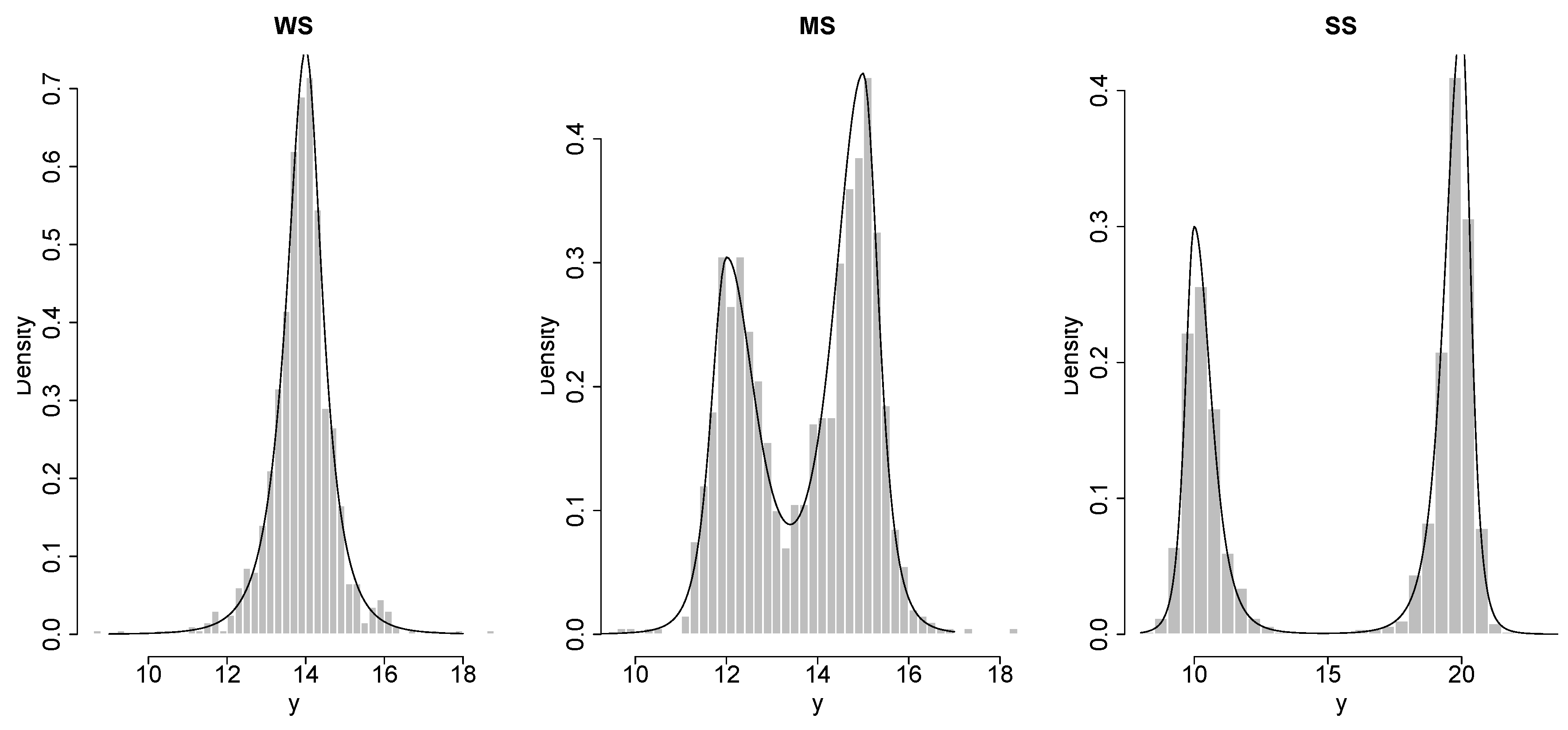
For this section, we simulated 400 samples each one with sample sizes , 600, 1000, 2000, 4000, from some FM-TP-T models with two components which are weak separated (WS), medium separated (MS) and strong separated (SS) of components, i.e., little, medium and large overlap of components respectively (see Figure 1), for which , , , , , , , and for WS data; for MS data; and for SS data.
Figure 1.
An artificial simulated finite mixture two-piece distributions based on the scale mixtures of normal (FM-TP-SMN) data of length with two components: weakly separated components (WS); medium separated components (MS) and strongly separated components (SS), with curved probability density function (PDF) that datasets extracted from them.
Using the proposed ECME algorithm to find the ML estimates we focus on the evaluation of Monte-Carlo average of biasness (MC-bias) and mean squared error (MSE) defined as of the ML estimates in each j-th sample, , respectively given in Table 3, Table 4 and Table 5 by
where is the ML estimate of the parameter in the i-th sample.

Table 3.
Monte-Carlo average bias (MC-bias) and mean squared error (MSE) for maximum likelihood (ML) estimates in the weak separated components (WS) FM-TP-true (T) model.

Table 4.
MC-Bias and MSE for ML estimates in the medium separated components (MS) FM-TP-T model.

Table 5.
MC-Bias and MSE for ML estimates estimates in the strong separated components (SS) FM-TP-T model.
These results in Table 3, Table 4 and Table 5 are obtained from the different fitted FM-TP-SMN models and show the performance of the proposed models as well as their parameters estimates. As the sample size increased we naturally observed that the Monte-Carlo average bias of ML estimates and MSE were tending toward zero.
4.2. Applications
In this section, we apply the FM-TP-SMN models on some various real data sets to show the performance of the proposed models and estimates in applications.
BMI Data
We considered the body mass index (BMI) data set collected for men aged between 18 and 80 years. The BMI data set was gathered with the National Health and Nutrition Examination Survey in the US National Center for Health Statistics (NCHS) of the Center for Disease Control (CDC). A strong relationship between the obesity problem and many chronic diseases has attracted attention in recent years, that is, most people with an obesity problem will have chronic diseases. The ratio of body weight in kilograms and height in squared meters (BMI) is a measure to determine the rate of relationship between overweight and obesity. In this way, a person with BMI > 25 is considered overweighed, while BMI > 30 is considered obese.
This dataset had 4579 participants with BMI records, but for modeling with finite mixture models, participants with weights within 39.50–70.00 kg and 95.01–196.80 kg with 1069 and 1054 participants were considered in the first and second subgroups respectively. Lin et al. [7] were first analyzed this dataset by considering the reports in 1999–2000 and 2001–2002, and were fitted the FM-normal, FM-T, FM-SN and FM-ST, always with two components, and then [5,13] fitted the FM-SMSN models to this dataset. The results, obtained by [13], were general and involved the results by [5,7]. So we fitted the proposed FM-TP-SMN models to this dataset and compared obtained results in the [13].
Table 6 contains the ML estimates of the FM-TP-SMN models with two components, and the Log-likelihood, AIC and BIC criterions of the proposed FM-TP-SMN models and FM-SMSN taken from Table 1 due to [13] appear in Table 7.

Table 6.
ML estimation results for fitting FM-TP-SMN models to the body mass index (BMI) data.

Table 7.
Model selection criteria for fitting FM-TP-SMN and FM-scale mixtures of the skew normal (SMSN) models to the BMI data. The best values are marked in bold.
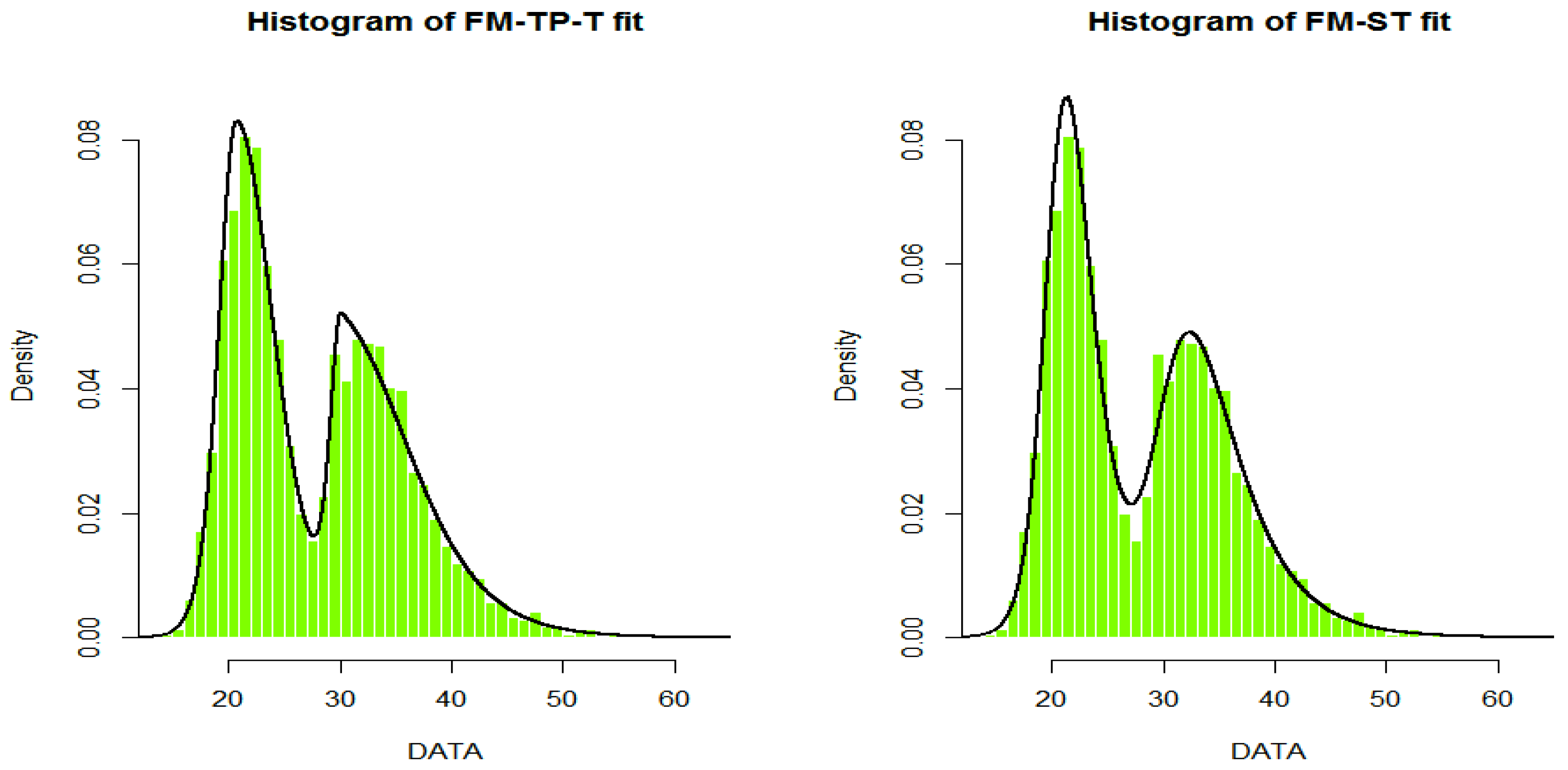
As noted by Lin et al. [4] and Prates et al. [13], the criteria values in Table 7 indicate that the heavy tailed FM-SMSN models (FM-ST, FM-SCN and FM-SSL) had a better fit than the ordinary FM-NOR and FM-SN models, and also the FM-SSL and FM-ST were the best fitted models. Such results are for the FM-TP-SMN (with corresponding FM-SMSN counterparts) models, while the FM-TP-SMN models were more reasonable than FM-TP-SMN models. However, the FM-TP-SL and FM-TP-T were the best models. In Figure 2, we plot the fitted FM-TP-T and FM-ST densities curved on the histogram of BMI data.
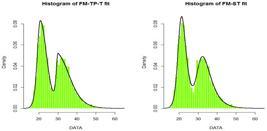
Figure 2.
Histogram of body mass index (BMI) data with fitted FM-TP-true (T) (left) and FM-ST (right) models with two components.
4.3. UScrime Data
As a further application of the FM-TP-SMN models and proposed methodology, we consider the effect of punishment regimes on crime rates [33,34], which is of high interest to criminologists. This has been studied using aggregate data of 47 US states for 1960 given in this data frame, and we consider the 13th column of this data frame which is due to income inequality. The data are available under the UScrime function in the MASS R package.
Table 8 contains the ML estimates of the FM-TP-SMN models with two components, and the Log-likelihood, AIC and BIC criterions of the proposed FM-TP-SMN and FM- SMSN models.

Table 8.
ML estimation results and model selection criteria for fitting FM-TP-SMN models to the UScrime data. The best values are marked in bold.
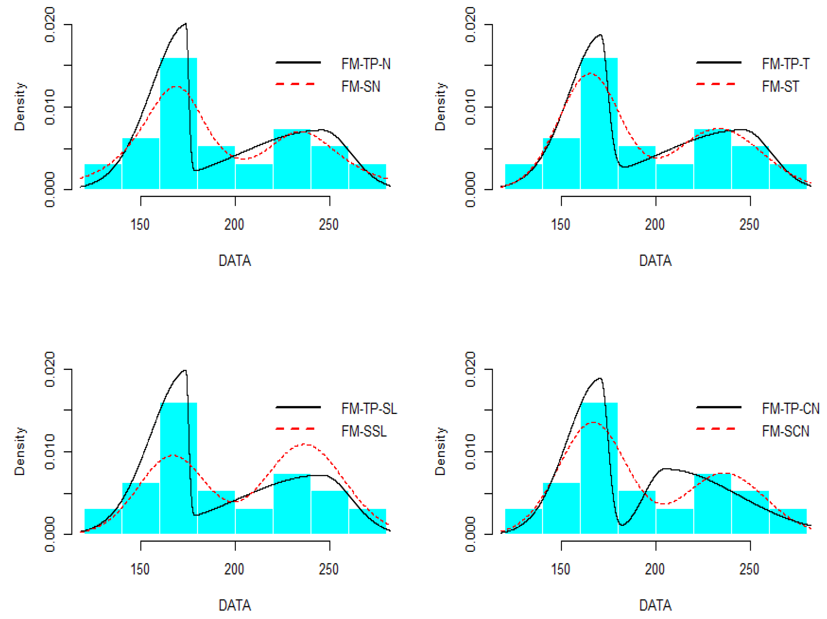
The log-likelihood values in Table 8 indicate that the FM-TP-N and FM-TP-T are the best models within the FM-TP-SMN models, while the FM-SCN is the best model in the class of the FM-SMSN models. The AIC and BIC criteria chose the FM-TP-N model (asymmetric components) within the FM-TP-SMN models, while they chose the FM-NOR model (symmetric components) in the class of the FM-SMSN models, which has symmetrical components. Among all competitors, the criteria chose the FM-TP-N model belonging to the proposed FM-TP-SMN models, which is more reasonable. In Figure 3 is plotted the histogram of US crime data with the curves of FM-TP-SMN and FM-SMSN models. These graphical visualizations show the suitability of the asymmetrical components and proposed FM-TP-SMN models.
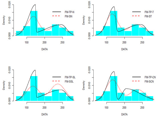
Figure 3.
Histogram of UScrime data with fitted FM-TP-SMN and FM-SMSN models with two components.
5. Conclusions
We have proposed a flexible family of TP-SMN distributions for application in clustering problems. The TP-SMN family is capable of representing distributions of symmetric/asymmetric and light/heavy tailed forms, which contains the well-known symmetric SMN family and is a reasonable competitor for asymmetric SMSN family as a special case. Estimation of the finite mixtures of the FM-TP-SMN parameters is relatively straightforward via the ECME algorithm with a fast convergence (a few iterations loop). Considering a Bayesian approach and the flexible TP-SMN family in the Autoregressive and ARMA processes from [35,36] can be further topics of research.
Author Contributions
M.M., J.E.C.-R. and M.R.M. wrote the paper and contributed the reagents/analysis/materials tools; M.M. conceived, designed, and performed the experiments, and analyzed the data. All authors read and approved the final manuscript. All authors have read and approved the final manuscript.
Acknowledgments
The authors thank the editor and three anonymous referees for their helpful comments and suggestions.
Conflicts of Interest
The authors declare that there is no conflict of interest in the publication of this paper.
References
- McLachlan, G.; Peel, D. Finite Mixture Models; John Wiley and Sons: New York, NY, USA, 2000. [Google Scholar]
- Contreras-Reyes, J.E.; Cortés, D.D. Bounds on Rényi and Shannon Entropies for Finite Mixtures of Multivariate Skew-Normal Distributions: Application to Swordfish (Xiphias gladius Linnaeus). Entropy 2016, 18, 382. [Google Scholar] [CrossRef]
- Frühwirth-Schnatter, S.; Pyne, S. Bayesian inference for finite mixtures of univariate and multivariate skew-normal and skew-t distributions. Biostatistics 2010, 11, 317–336. [Google Scholar] [CrossRef] [PubMed]
- Lin, T.I.; Lee, J.C.; Yen, S.Y. Finite mixture modelling using the skew normal distribution. Stat. Sin. 2007, 17, 909–927. [Google Scholar]
- Basso, R.M.; Lachos, V.H.; Cabral, C.R.B.; Ghosh, P. Robust mixture modeling based on scale mixtures of skew-normal distributions. Comput. Stat. Data Anal. 2010, 54, 2926–2941. [Google Scholar] [CrossRef]
- Lin, T.I. Robust mixture modeling using multivariate skew t distributions. Stat. Comput. 2009, 20, 343–356. [Google Scholar] [CrossRef]
- Lin, T.I.; Lee, J.C.; Hsieh, W.J. Robust Mixture Modelling Using the Skew t Distribution. Stat. Comput. 2007, 17, 81–92. [Google Scholar] [CrossRef]
- Contreras-Reyes, J.E.; López Quintero, F.O.; Yáñez, A.A. Towards Age Determination of Southern King Crab (Lithodes santolla) Off Southern Chile Using Flexible Mixture Modeling. J. Mar. Sci. Eng. 2018, 6, 157. [Google Scholar] [CrossRef]
- Maleki, M.; Arellano-Valle, R.B. Maximum a-posteriori estimation of autoregressive processes based on finite mixtures of scale-mixtures of skew-normal distributions. J. Stat. Comput. Sim. 2017, 87, 1061–1083. [Google Scholar] [CrossRef]
- Maleki, M.; Arellano-Valle, R.B.; Dey, D.K.; Mahmoudi, M.R.; Jalali, S.M.J. A Bayesian Approach to Robust Skewed Autoregressive Processes. Calcutta Stat. Assoc. Bull. 2017, 69, 165–182. [Google Scholar] [CrossRef]
- Maleki, M.; Wraith, D.; Arellano-Valle, R.B. Robust finite mixture modeling of multivariate unrestricted skew-normal generalized hyperbolic distributions. Stat. Comput. 2018, in press. [Google Scholar] [CrossRef]
- Maleki, M.; Wraith, D.; Arellano-Valle, R.B. A flexible class of parametric distributions for Bayesian linear mixed models. Test 2018, in press. [Google Scholar] [CrossRef]
- Prates, M.O.; Lachos, V.H.; Cabral, C. mixsmsn: Fitting finite mixture of scale mixture of skew-normal distributions. J. Stat. Soft. 2000, 54, 1–20. [Google Scholar] [CrossRef]
- Hajrajabi, A.; Maleki, M. Nonlinear semiparametric autoregressive model with finite mixtures of scale mixtures of skew normal innovations. J. Appl. Stat. 2019, in press. [Google Scholar] [CrossRef]
- Maleki, M.; Wraith, D. Mixtures of multivariate restricted skew-normal factor analyzer models in a Bayesian framework. Comput. Stat. 2019, in press. [Google Scholar] [CrossRef]
- Andrews, D.R.; Mallows, C.L. Scale mixture of normal distribution. J. R. Stat. Soc. Ser. B 1974, 36, 99–102. [Google Scholar] [CrossRef]
- Lange, K.L.; Little, R.; Taylor, J. Robust statistical modeling using t distribution. J. Am. Stat. Assoc. 1989, 84, 881–896. [Google Scholar] [CrossRef]
- Lange, K.L.; Sinsheimer, J.S. Normal/independent distributions and their applications in robust regression. J. Comput. Graph. Stat. 1993, 2, 175–198. [Google Scholar]
- Maleki, M.; Nematollahi, A.R. Autoregressive Models with Mixture of Scale Mixtures of Gaussian innovations. Iranian J. Sci. Technol. Trans. A 2017, 41, 1099–1107. [Google Scholar] [CrossRef]
- Arellano-Valle, R.B.; Gómez, H.; Quintana, F.A. Statistical inference for a general class of asymmetric distributions. J. Stat. Plan. Inf. 2005, 128, 427–443. [Google Scholar] [CrossRef]
- Hoseinzadeh, A.; Maleki, M.; Khodadadi, Z.; Contreras-Reyes, J.E. The Skew-Reflected-Gompertz distribution for analyzing symmetric and asymmetric data. J. Comput. Appl. Math. 2019, 349, 132–141. [Google Scholar] [CrossRef]
- Moravveji, B.; Khodadai, Z.; Maleki, M. A Bayesian Analysis of Two-Piece distributions based on the Scale Mixtures of Normal Family. Iranian J. Sci. Technol. Trans. A 2018, in press. [Google Scholar] [CrossRef]
- Maleki, M.; Mahmoudi, M.R. Two-Piece Location-Scale Distributions based on Scale Mixtures of Normal family. Commun. Stat. Theor. Meth. 2017, 46, 12356–12369. [Google Scholar] [CrossRef]
- Rubio, F.J.; Steel, M.F.G. Inference in Two-Piece Location-Scale Models with Jeffreys Priors. Bayesian Anal. 2014, 9, 1–22. [Google Scholar] [CrossRef]
- Branco, M.D.; Dey, D.K. A general class of multivariate skew-elliptical distributions. J. Multivar. Anal. 2001, 79, 99–113. [Google Scholar] [CrossRef]
- Mudholkar, G.S.; Hutson, A.D. The epsilon-skew-normal distribution for analyzing near-normal data. J. Stat. Plan. Inf. 2000, 83, 291–309. [Google Scholar] [CrossRef]
- Meng, X.; Rubin, D.B. Maximum likelihood estimation via the ECM algorithm: A general framework. Biometrika 2017, 80, 267–278. [Google Scholar] [CrossRef]
- Dempster, A.P.; Laird, N.M.; Rubin, D.B. Maximum likelihood from incomplete data via the EM algorithm. J. R. Stat. Soc. Ser. B 1977, 39, 1–38. [Google Scholar] [CrossRef]
- Liu, C.; Rubin, D.B. The ECME algorithm: A simple extension of EM and ECM with faster monotone convergence. Biometrika 1994, 81, 633–648. [Google Scholar] [CrossRef]
- R Core Team. A Language and Environment for Statistical Computing; R Foundation for Statistical Computing: Vienna, Austria, 2018; ISBN 3-900051-07-0. Available online: http://www.R-project.org (accessed on 12 December 2018).
- Akaike, H. A new look at the statistical model identification. IEEE Trans. Autom. Control 1974, 19, 716–723. [Google Scholar] [CrossRef]
- Schwarz, G. Estimating the dimension of a model. Ann. Stat. 1978, 6, 461–464. [Google Scholar] [CrossRef]
- Ehrlich, I. Participation in illegitimate activities: A theoretical and empirical investigation. J. Political Econ. 1973, 81, 521–565. [Google Scholar] [CrossRef]
- Vandaele, W. Participation in illegitimate activities: Ehrlich revisited. In Deterrence and Incapacitation; Blumstein, A., Cohen, J., Nagin, D., Eds.; US National Academy of Sciences: Washington, DC, USA, 1978; pp. 270–335. [Google Scholar]
- Ghasami, S.; Khodadadi, Z.; Maleki, M. Autoregressive Processes with Generalized Hyperbolic Innovations. Commun. Stat. Comput. Sim. 2019, in press. [Google Scholar] [CrossRef]
- Zarrin, P.; Maleki, M.; Khodadadi, Z.; Arellano-Valle, R.B. Time series process based on the unrestricted skew normal process. J. Stat. Comput. Sim. 2019, 89, 38–51. [Google Scholar] [CrossRef]
© 2019 by the authors. Licensee MDPI, Basel, Switzerland. This article is an open access article distributed under the terms and conditions of the Creative Commons Attribution (CC BY) license (http://creativecommons.org/licenses/by/4.0/).

