On the Numerical Solution of Ordinary, Interval and Fuzzy Differential Equations by Use of F-Transform

Abstract

An interesting property of the inverse F-transform $\widehat{f}$ of a continuous function f on a given interval $[a,b]$ says that the integrals of $\widehat{f}$ and f on $[a,b]$ coincide. Furthermore, the same property can be established for the restrictions of the functions to all subintervals $[a,p_k]$ of the fuzzy partition of $[a,b]$ used to define the F-transform. Based on this fact, we propose a new method for the numerical solution of ordinary differential equations (initial-value ordinary differential equation (ODE)) obtained by approximating the derivative $\stackrel{·}{x}\left(t\right)$ via F-transform, then computing (an approximation of) the solution $x\left(t\right)$ by exact integration. For an ODE, a global second-order approximation is obtained. A similar construction is then applied to interval-valued and (level-wise) fuzzy differential equations in the setting of generalized differentiability (gH-derivative). Properties of the new method are analyzed and a computational section illustrates the performance of the obtained procedures, in comparison with well-known efficient algorithms.

1. Introduction

The fuzzy transform (F-transform) of a continuous function $f:[a,b]⟶\mathbb{R}$ was introduced by Perfilieva in [1,2]. This special fuzzy method is particularly appealing and useful to handle many real-world problems and an extensive research activity has both analyzed its properties and its fields of applications; for the literature related to this paper we refer to, e.g., [3,4,5,6,7,8,9,10,11] and the references therein.

In recent research, attention has been paid to the numerically approximated solutions of ordinary differential equations (ODEs) $\stackrel{·}{x}\left(t\right)=F(t,x)$ of various types. In particular, it is shown that by using the inverse F-transform, it is possible to obtain good approximations of the solution $x\left(t\right)$. The methods that use the F-transform are (computationally) superior with respect to other ones such as the second-order Runge–Kutta algorithm or basic multi-step algorithms (see [12,13,14,15,16]). In the final section of this paper, we will present some comments and a preliminary comparative valuation of the proposed methods.

In this paper, we propose a numerical method where the inverse F-transform is used to approximate the derivative $\stackrel{·}{x}\left(t\right)$; the solution $x\left(t\right)$ is then obtained by exact integration of the approximated derivative: this is allowed by an interesting property which says that the integral of the inverse F-transform of f on $[a,b]$ coincides (exactly) with the integral of the function f itself; this idea was presented in a preliminary form in [17].

For an ordinary differential equation, including the case of a system, a global second-order approximation is obtained. Properties of the new method are analyzed and a computational section illustrates the performance of the obtained procedures, in comparison with well-known efficient algorithms.

A similar construction is then applied to interval-valued (IDE) and (level-wise) fuzzy differential equations (FDE) in the setting of generalized differentiability (gH-derivative, see [18,19,20]). IDEs and FDEs are designed to model uncertainty and its propagation in a dynamical setting and it is well known that the fuzzy case can be expressed in terms of a family of IDEs by adopting the level-wise representation of fuzzy numbers and fuzzy-valued functions. For a modern introduction to FDEs under Hukuhara and generalized derivative, we refer to chapter 9 of Bede’s book [21]. The interested reader is also referred to the recent book [22], in particular to chapter 4, and the references therein.

This paper is organized into five sections. In Section 2 we recall some of the basic definitions and properties of the F-transform as contained in [1,2,23]. Then, in Section 3, we describe our approach to the numerical solution of ordinary (and systems of) differential equations with initial conditions, usually referred as Cauchy problem. The F-transform is used to approximate the derivative of the solution to be founded and the unknown function is determined by point-wise by exact integration of the derivative; this section also contains the main properties of the method and a proof of its (global) convergence. Numerical examples and a computational comparison with other well-performing algorithms is presented in Section 4. Section 5 considers the case of interval differential equations and extends the use of F-transform to the numerical solution of IDEs and FDEs under (level-wise) generalized Hukuhara differentiability; in particular, the switching phenomenon is analyzed and rule to manage the switching is proposed and implemented in the proposed procedure. Several computational examples of interval and fuzzy differential equation are presented and discussed in Section 6. Section 7 presents some conclusions and present some ideas for further work.

2. Preliminaries

We briefly recall the basic definitions and properties of the F-transform setting. For all the details, we refer to the papers [1,2,23].

A fuzzy partition $(\mathbb{P},\mathbb{A})$ of the compact interval $[a,b]$ is defined by a finite decomposition $\mathbb{P}=\{a=p_1<p_2<\dots <p_n=b\}$ of $[a,b]$ with n points and by a family $\mathbb{A}=\{A_1,A_2,\dots ,A_n\}$ of n continuous basic functions $A_k:[a,b]⟶[0,1]$ with the following properties (the decomposition $\mathbb{P}$ is not required to be uniform):

• $A_k\left(t\right)=0$ for $t\notin ]p_{k-1},p_{k+1}[$ ($k=2,\dots ,n-1$), $A_1\left(t\right)=0$ for $t\notin [p_1,p_2[$, $A_n\left(t\right)=0$ for $t\notin ]p_{n-1},p_n]$;
• $A_k\left(p_k\right)=1$ for all $k=1,2,\dots ,n$ and $A_1\left(t\right)+A_2\left(t\right)+\dots +A_n\left(t\right)=1$ for all $t\in [a,b]$;
• for $k=2,\dots ,n-1$, $A_k$ is increasing on $[p_{k-1},p_k]$ and decreasing on $[p_k,p_{k+1}]$, $A_1$ is decreasing on $[p_1,p_2]$, $A_n$ is increasing of $[p_{n-1},p_n]$.

Let us define the following integrals

$$\left\{\begin{array}{ccc}{I}_1^{-}=0\hfill & ,\hfill & I_1^{+}={\int }_{p_1}^{p_2}{A}_1\left(t\right)dt\hfill \\ I_k^{-}={\int }_{p_{k-1}}^{p_k}{A}_k\left(t\right)dt\hfill & ,\hfill & I_k^{+}={\int }_{p_k}^{p_{k+1}}{A}_k\left(t\right)dt\hfill \\ I_n^{-}={\int }_{p_{n-1}}^{p_n}{A}_1\left(t\right)dt\hfill & ,\hfill & I_n^{+}=0\hfill \end{array}\right.$$

(1)

and

$$I_k=I_k^{-}+I_k^{+}\mathrm{for}k=1,\dots ,n.$$

(2)

The direct F-transform of f with respect to $(\mathbb{P},\mathbb{A})$ is the n-tuple of real numbers ${\mathbf{F}}_{(\mathbb{P},\mathbb{A})}=(F_1,F_2,\dots ,F_n)$ defined as

$$\begin{array}{cc}\hfill F_1& =\frac{1}{I_1}\underset{p_1}{\overset{p_2}{\int }}f\left(t\right)A_k\left(t\right)dt,F_n=\frac{1}{I_n}\underset{p_1}{\overset{p_n}{\int }}f\left(t\right)A_k\left(t\right)dt,\hfill \\ \hfill F_k& =\frac{1}{I_k}\underset{p_{k-1}}{\overset{p_{k+1}}{\int }}f\left(t\right)A_k\left(t\right)dt,k=2,\dots ,n-1\hfill \end{array}$$

(3)

and, obtained from the direct fuzzy transform ${\mathbf{F}}_{(\mathbb{P},\mathbb{A})}$, the inverse F-transform (iF-transform) of f is the function $f_{(\mathbb{P},\mathbb{A})}:[a,b]⟶R$ given by

$$f_{(\mathbb{P},\mathbb{A})}\left(t\right)={\displaystyle \sum _{k=1}^n}{F}_k{A}_k\left(t\right)\mathrm{for}t\in [a,b].$$

(4)

The following properties (see [1]) are the fundamentals of the F-transform setting.

Proposition 1.

(from [1]) If $f:[a,b]⟶\mathbb{R}$ is a continuous function then;

 1. 

for any positive real ε, there exists a fuzzy partition $({\mathbb{P}}_{\epsilon },{\mathbb{A}}_{\epsilon })$ such that the corresponding iF-transform $f_{({\mathbb{P}}_{\epsilon },{\mathbb{A}}_{\epsilon })}:[a,b]⟶\mathbb{R}$ satisfy

$$\left|f\left(t\right)-f_{({\mathbb{P}}_{\epsilon },{\mathbb{A}}_{\epsilon })}\left(t\right)\right|<\epsilon forallt\in [a,b].$$

 2. 

for all $k=1,\dots ,n$,

$$\begin{array}{cc}\hfill F_k& =f_{(\mathbb{P},\mathbb{A})}\left(p_k\right)\hfill \end{array}$$

(5)

$$\begin{array}{cc}\hfill f\left(p_k\right)& =F_k+O\left(h^2\right)ash⟶0\hfill \end{array}$$

(6)

where $h=max\{p_{k+1}-p_k;k=1,\dots ,n-1\}$.

 3. 

the direct and inverse F-transforms are linear, i.e., for any $\lambda \in \mathbb{R}$ and for any two continuous functions $f,g:[a,b]⟶\mathbb{R}$, with direct F-transforms ${\mathbf{F}}_{(\mathbb{P},\mathbb{A})}$ and ${\mathbf{G}}_{(\mathbb{P},\mathbb{A})}$ with respect to the same partition $(\mathbb{P},\mathbb{A})$; then

 3.1. 

the direct F-transforms of $\lambda f$ and $f+g$ are, respectively, $\lambda {\mathbf{F}}_{(\mathbb{P},\mathbb{A})}$ and ${\mathbf{F}}_{(\mathbb{P},\mathbb{A})}+{\mathbf{G}}_{(\mathbb{P},\mathbb{A})}$,

 3.2. 

the inverse F-transform of $\lambda f$ and $f+g$ are, respectively,$\lambda f_{(\mathbb{P},\mathbb{A})}$ and $f_{(\mathbb{P},\mathbb{A})}+g_{(\mathbb{P},\mathbb{A})}$.

In [10], the following property has been established:

Proposition 2.

Let $f,g:[a,b]⟶\mathbb{R}$ be continuous functions and let $(\mathbb{P},\mathbb{A})$ be a fuzzy partition of $[a,b]$. Then

 (i) 

the iF-transform satisfies

$$\underset{a}{\overset{b}{\int }}{f}_{(\mathbb{P},\mathbb{A})}\left(t\right)dt=\underset{a}{\overset{b}{\int }}f\left(t\right)dt$$

(7)

 (ii) 

if f ang g have the same direct F-transform components ${\mathbf{F}}_{(\mathbb{P},\mathbb{A})}={\mathbf{G}}_{(\mathbb{P},\mathbb{A})}$, then

$${\int }_a^{b}f\left(t\right)dt={\int }_a^{b}g\left(t\right)dt.$$

It is interesting to observe that a fuzzy partition has a “nesting” property (its proof is immediate):

Proposition 3.

Let $(\mathbb{P},\mathbb{A})$ be a fuzzy partition of interval $[a,b]$ with $\mathbb{P}=\left\{a=p_1<p_2<\dots <p_n=b\right\}$ and consider any subinterval $[a,p_k]$ with $k=2,\dots ,n$; let $({\mathbb{P}}_k,{\mathbb{A}}_k)$ be the fuzzy partition of $[a,p_k]$ defined by

$$\begin{array}{cc}\hfill {\mathbb{P}}_k& =\{a,p_2,\dots ,p_k\}\hfill \\ \hfill {\mathbb{A}}_k& =\{A_1,\dots ,{\tilde{A}}_k\}\hfill \end{array}$$

(8)

where the last basic function ${\tilde{A}}_k$ is given by the restriction of the basic function $A_k$ to the subinterval $[p_{k-1},p_k]$. The fuzzy partition $({\mathbb{P}}_k,{\mathbb{A}}_k)$, $k=1,2,\dots ,n$ is called the k-th nested partition associated with $(\mathbb{P},\mathbb{A})$ and clearly $({\mathbb{P}}_n,{\mathbb{A}}_n)=(\mathbb{P},\mathbb{A})$.

A consequences of the properties above is the following proposition:

Proposition 4.

Let $f:[a,b]⟶\mathbb{R}$ be a continuous function and let ${\mathit{F}}_{(\mathbb{P},\mathbb{A})}={(F_1,F_2,\dots ,F_n)}^T$ be its F-transform with respect to $(\mathbb{P},\mathbb{A})$. Then, for any $k=2,\dots ,n-1$, the F-transform of the restriction of f to the subinterval $[a,p_k]$ (with respect to the k-th nested partition $({\mathbb{P}}_k,{\mathbb{A}}_k)$), is given by ${\mathit{F}}^{\left(k\right)}={(F_1,\dots ,F_{k-1},{\tilde{F}}_k)}^T$ where only the last component ${\tilde{F}}_k$ is changed with respect to the components in ${\mathit{F}}_{(\mathbb{P},\mathbb{A})}$ and is given by

$${\tilde{F}}_k=\frac{\underset{a}{\overset{p_k}{\int }}f\left(t\right)A_k\left(t\right)dt}{\underset{a}{\overset{p_k}{\int }}{A}_k\left(t\right)dt}.$$

(9)

We have, for all $k=2,\dots ,n-1$ (the central summation is assumed to be zero if $k=2$),

$$f_{({\mathbb{P}}_k,{\mathbb{A}}_k)}\left(t\right)=F_1{A}_1\left(t\right)+{\displaystyle \sum _{j=2}^{k-1}}{F}_j{A}_j\left(t\right)+{\tilde{F}}_k{\tilde{A}}_k\left(t\right)$$

and

$$\underset{a}{\overset{p_k}{\int }}f\left(t\right)dt=F_1\underset{a}{\overset{p_k}{\int }}{A}_1\left(t\right)dt+{\displaystyle \sum _{j=2}^{k-1}}{F}_j\underset{a}{\overset{p_{j+1}}{\int }}{A}_j\left(t\right)dt+{\tilde{F}}_k\underset{a}{\overset{p_k}{\int }}{A}_k\left(t\right)dt.$$

(10)

With the notation in (1), equality (10) is written (for $k>1$) as

$$\underset{a}{\overset{p_k}{\int }}f\left(t\right)dt=F_1{I}_1^{+}+{\displaystyle \sum _{j=2}^{k-1}}{F}_j{I}_j+{\tilde{F}}_k{I}_k^{-}$$

(11)

and we have:

Proposition 5.

Let $f:[a,b]⟶\mathbb{R}$ be a continuous function, let $(\mathbb{P},\mathbb{A})$ be a uniform fuzzy partition of $[a,b]$ with $h=\frac{b-a}{n-1}$ and let ${\mathit{F}}_{(\mathbb{P},\mathbb{A})}={(F_1,F_2,\dots ,F_n)}^T$ be the F-transform of f; let also ${\mathit{F}}^{\left(k\right)}={(F_1,\dots ,F_{k-1},{\tilde{F}}_k)}^T$ be as in (9) for any $k=2,\dots ,n-1$. Then

$$\begin{array}{cc}\hfill I_k^{-}{\tilde{F}}_k& =\frac{h}{2}f\left(p_k\right)+O\left(h^3\right)ash⟶0\hfill \\ \hfill I_k{F}_k& =hf\left(p_k\right)+O\left(h^3\right)ash⟶0.\hfill \end{array}$$

Proof. 

Consider $2\le k\le n-1$. We have $I_k^{-}{\tilde{F}}_k=\underset{p_{k-1}}{\overset{p_k}{\int }}f\left(t\right)A_k\left(t\right)dt$ and, by the trapezoidal integration,

$$I_k^{-}{\tilde{F}}_k=\frac{h}{2}[f\left(p_{k-1}\right)A_k\left(p_{k-1}\right)+f\left(p_k\right)A_k\left(p_k\right)]+O\left(h^3\right);$$

on the other hand, $A_k\left(p_k\right)=1$ and $A_k\left(p_{k-1}\right)=0$, so $I_k^{-}{\tilde{F}}_k=\frac{h}{2}f\left(p_k\right)+O\left(h^3\right)$. For the second equality (consider that $A_k\left(p_{k+1}\right)=0$) we have

$$\begin{array}{cc}\hfill I_k{F}_k& =I_k^{-}{\tilde{F}}_k+\frac{h}{2}f\left(p_k\right)+O\left(h^3\right)\hfill \\ \hfill & =\frac{h}{2}f\left(p_k\right)+\frac{h}{2}f\left(p_k\right)+O\left(h^3\right)=hf\left(p_k\right)+O\left(h^3\right).\hfill \end{array}$$

 □

3. Numerical Solution of Initial-Value ODE by F-Transform

Let us consider the following initial-value ordinary differential equation (ODE):

$$\left\{\begin{array}{c}\stackrel{·}{x}\left(t\right)=f\left(t,x\left(t\right)\right),t\in \left[t_0,t_1\right]\hfill \\ x\left(t_0\right)=x_0\hfill \end{array}\right.$$

(12)

We assume the usual requirements on function $f(t,x)$ that ensure existence and unicity of the solution $x\left(t\right)$, $t\in \left[t_0,t_1\right]$.

We are interested to find an approximation of the final value $x\left(t_1\right)$ of the solution $x\left(t\right)$. Let $(\mathbb{P},\mathbb{A})$ be a fixed (but arbitrary) uniform fuzzy partition of $\left[t_0,t_1\right]$ with $p_1=t_0$, $p_k=p_{k-1}+h$, $k=2,\dots ,n$ and $h=\frac{t_1-t_0}{n-1}$; let $\mathbb{A}=\left\{A_1,\dots ,A_n\right\}$ be the basic functions. Let ${\stackrel{·}{x}}_{(\mathbb{P},\mathbb{A})}$ denote the iF-transform of $\stackrel{·}{x}\left(t\right)$ with (exact) direct F-transform components ${\left(F_k\right)}_{k=1,\dots ,n}$.

In the rest of the paper, we will make use of the following functions and notation: for any basic function $A_k\in \mathbb{A}$, $k=1,2,\dots ,n$, we will denote by $B_k$ the integral function defined by

$$B_k\left(t\right)={\int }_{t_0}^t{A}_k\left(s\right)ds.$$

The components of the direct F-transform of $\stackrel{·}{x}\left(t\right)$ will be denoted by $F_1,F_2,\dots ,F_n$ and the inverse F-transform of ${\stackrel{·}{x}}_{(\mathbb{P},\mathbb{A})}$ of is the function

$${\stackrel{·}{x}}_{(\mathbb{P},\mathbb{A})}\left(t\right)={\displaystyle \sum _{k=1}^n}{F}_k{A}_k\left(t\right)\mathrm{for}t\in [a,b].$$

(13)

The following proposition follows immediately from (10).

Proposition 6.

If the exact values ${\left(F_k\right)}_{k=1,\dots ,n}$ of the direct F-transform components of the function $t⟶f\left(t,x\left(t\right)\right)$ on $\left[t_0,t_1\right]$ with respect to the fuzzy partition $(\mathbb{P},\mathbb{A})$ are known, then the final value $x\left(t_1\right)$ of the solution of (12) is exactly given by

$$x\left(t_1\right)=x_0+{\displaystyle \sum _{k=1}^n}{F}_k{I}_k.$$

Furthermore, at the intermediate points $p_k$, $k=2,\dots ,n-1$ of the decomposition $\mathbb{P}$, we have that the solution $x\left(p_k\right)$ is exactly given by

$$x\left(p_k\right)=x_0+{\displaystyle \sum _{j=1}^{k-1}}{F}_j{I}_j+{\tilde{F}}_k{I}_k^{-}$$

(14)

Proof. 

By definition, we have

$${\stackrel{·}{x}}_{(\mathbb{P},\mathbb{A})}\left(t\right)={\displaystyle \sum _{k=1}^n}{F}_k{A}_k\left(t\right)$$

and, from property (ii) in Proposition 1, also

$${\int }_{t_0}^{t_1}{\stackrel{·}{x}}_{(\mathbb{P},\mathbb{A})}\left(t\right)dt={\int }_{t_0}^{t_1}\stackrel{·}{x}\left(t\right)dt;$$

we then obtain

$$x\left(t_1\right)=x_0+{\int }_{t_0}^{t_1}{\stackrel{·}{x}}_{(\mathbb{P},\mathbb{A})}\left(s\right)ds=x_0+{\displaystyle \sum _{k=1}^n}{F}_k{B}_k\left(t_1\right).$$

By Proposition 2 applied to the derivative function $\stackrel{·}{x}\left(t\right)=f\left(t,x\left(t\right)\right)$, with $(\mathbb{P},\mathbb{A})$ on $\left[t_0,t_1\right]$, and using (1)–(2), we have $B_j\left(p_k\right)=I_j$ and $B_k\left(p_k\right)=I_k^{-}$ and the conclusion follows.  □

Remark 1.

Consider that in general we have $x\left(t\right)\ne$$x_0+{\int }_{t_0}^t{\stackrel{·}{x}}_{(\mathbb{P},\mathbb{A})}\left(s\right)ds$, for $t\notin \{p_1,\dots ,p_n\}$.

From the properties of F-transform as in Proposition 1 (point 3.) we finally have the following

Proposition 7.

If the exact values ${\left(F_k\right)}_{k=1,\dots ,n}$ of the direct F-transform components of the function $t⟶f\left(t,x\left(t\right)\right)$ on $\left[t_0,t_1\right]$ with respect to a fuzzy partition $(\mathbb{P},\mathbb{A})$ are known, then the solution $x\left(t\right)$ of (12), for all $k=1,\dots ,n-1$, satisfies

$$x\left(t\right)=x_{(\mathbb{P},\mathbb{A},x_0)}\left(p_k\right)+{\int }_{p_k}^{t}f\left(s,x\left(s\right)\right)ds,oorallt\in [p_k,p_{k+1}[,$$

where

$$x_{(\mathbb{P},\mathbb{A},x_0)}\left(t\right)=x_0+{\int }_{t_0}^t{\stackrel{·}{x}}_{(\mathbb{P},\mathbb{A})}\left(s\right)ds$$

(15)

Proof. 

Apply the identity $x\left(t\right)=x_0+{\int }_{t_0}^{p_k}f\left(s,x\left(s\right)\right)ds$$+{\int }_{p_k}^{t}f\left(s,x\left(s\right)\right)ds$ and (14).  □

3.1. An F-Transform Algorithm for ODE

In view of Propositions 6 and 7, we then need a way to compute or to approximate the direct F-transform components ${\left(F_k\right)}_{k=1,\dots ,n}$ of $\stackrel{·}{x}\left(t\right)$.

By definition, we have that (here $p_0=p_1$ and $p_{n+1}=p_n$), for $k=1,2,\dots ,n$,

$$\begin{array}{cc}\hfill I_k{F}_k& ={\int }_{p_{k-1}}^{p_{k+1}}\stackrel{·}{x}\left(t\right)A_k\left(t\right)dt={\int }_{p_{k-1}}^{p_{k+1}}f(t,x\left(t\right))A_k\left(t\right)dt\hfill \\ \hfill I_k^{-}{\tilde{F}}_k& ={\int }_{p_{k-1}}^{p_k}\stackrel{·}{x}\left(t\right)A_k\left(t\right)dt={\int }_{p_{k-1}}^{p_k}f(t,x\left(t\right))A_k\left(t\right)dt\hfill \end{array}$$

and, from Proposition 5,

$$\begin{array}{cc}\hfill I_k{F}_k& =hf(p_k,x\left(p_k\right))+O\left(h^3\right)\hfill \\ \hfill I_k^{-}{\tilde{F}}_k& =\frac{h}{2}f(p_k,x\left(p_k\right))+O\left(h^3\right).\hfill \end{array}$$

As a final step, substitute $x\left(p_k\right)=$$x_0+{\displaystyle \sum _{j=1}^{k-1}}{F}_j{I}_j+{\tilde{F}}_k{I}_k^{-}$ and obtain, for $h⟶0$,

$$\begin{array}{cc}\hfill I_k{F}_k& =hf\left(p_k,x_0+{\displaystyle \sum _{j=1}^{k-1}}{F}_j{I}_j+{\tilde{F}}_k{I}_k^{-}\right)+O\left(h^3\right)\hfill \end{array}$$

(16)

$$\begin{array}{cc}\hfill I_k^{-}{\tilde{F}}_k& =\frac{h}{2}f\left(p_k,x_0+{\displaystyle \sum _{j=1}^{k-1}}{F}_j{I}_j+{\tilde{F}}_k{I}_k^{-}\right)+O\left(h^3\right).\hfill \end{array}$$

(17)

Approximated values $G_k$ and ${\tilde{G}}_k$ of $F_k$ and ${\tilde{F}}_k$, respectively, can be computed by solving the following equations (we will assume that the sums below will be zero if $k=1$)

$$\begin{array}{cc}\hfill I_k{G}_k& =hf\left(p_k,x_0+{\displaystyle \sum _{j=1}^{k-1}}{G}_j{I}_j+{\tilde{G}}_k{I}_k^{-}\right)\hfill \end{array}$$

(18)

$$\begin{array}{cc}\hfill I_k^{-}{\tilde{G}}_k& =\frac{h}{2}f\left(p_k,x_0+{\displaystyle \sum _{j=1}^{k-1}}{G}_j{I}_j+{\tilde{G}}_k{I}_k^{-}\right).\hfill \end{array}$$

(19)

To solve Equations (18) and (19) let us write them for different values of $k=1,\dots ,n$. The first component $G_1$ can be determined from the initial condition $\stackrel{·}{x}\left(t_0\right)=f(t_0,x\left(t_0\right))=f(p_1,x_0)$, obtained from $I_1{F}_1=hf(p_1,x\left(p_1\right))+O\left(h^3\right)$ by ignoring the term $O\left(h^3\right)$:

$$G_1=\frac{hf(t_0,x_0)}{I_1}.$$

(20)

When computing $G_2$ and ${\tilde{G}}_2$, the value of $G_1$ is known, and Equations (18) and (19) become

$$\begin{array}{cc}\hfill I_2^{-}{\tilde{G}}_2& =\frac{h}{2}f\left(p_2,x_0+G_1{I}_1+{\tilde{G}}_2{I}_2^{-}\right)\hfill \end{array}$$

(21)

$$\begin{array}{cc}\hfill I_2{G}_2& =hf\left(p_2,x_0+G_1{I}_1+{\tilde{G}}_2{I}_2^{-}\right).\hfill \end{array}$$

(22)

From the first equation we determine ${\tilde{G}}_2$ and, by substituting into the second, we compute $G_2=2I_2^{-}{\tilde{G}}_2/I_2$.

For a general $k,$ the values $G_1,\dots ,G_{k-1}$ are known and we need to solve Equation (19) only for ${\tilde{G}}_k$

$$I_k^{-}{\tilde{G}}_k=\frac{h}{2}f\left(p_k,x_0+{\displaystyle \sum _{j=1}^{k-1}}{G}_j{I}_j+{\tilde{G}}_k{I}_k^{-}\right);$$

(23)

then we set $G_k=2I_k^{-}{\tilde{G}}_k/I_k$.

Summarizing, we determine the values ${\tilde{G}}_k$ and $G_k$ iteratively from (23) starting with (20). Each Equation (23) has the form of a fixed-point problem for ${\tilde{G}}_k$

$${\tilde{G}}_k=\frac{h}{2I_k^{-}}f\left(p_k,x_0+{\displaystyle \sum _{j=1}^{k-1}}{G}_j{I}_j+{\tilde{G}}_k{I}_k^{-}\right)$$

and can be solved by any zero finder routine or, considering that the system is in (nonlinear) triangular form, by any iterative procedure.

We have the following approximation property for the solution of (12).

Theorem 1.

Let $G_k=(G_1,\dots ,G_{k-1},{\tilde{G}}_k)$ be solutions of (20)–(23) and define

$$x_{{\mathbb{G}}_k}\left(p_k\right)=x_0+{\displaystyle \sum _{j=1}^{k-1}}{G}_j{I}_j+{\tilde{G}}_k{I}_k^{-}\mathrm{for}k=1,2,\dots ,n.$$

Then, for the solution $x\left(p_k\right)$ of (12) at the points $p_k$, $k=1,2,\dots ,n$, we have

$$\begin{array}{cc}\hfill x\left(p_k\right)& =x_{{\mathbb{G}}_k}\left(p_k\right)+O\left(k{h}^3\right)\mathit{as}h⟶0,\hfill \\ \hfill x\left(t_1\right)& =x_{{\mathbb{G}}_n}\left(t_1\right)+(t_1-t_0)O\left(h^2\right)\mathit{as}h⟶0.\hfill \end{array}$$

Proof. 

From (14), (24) and (25) we have

$$\begin{array}{cc}\hfill |x\left(p_k\right)-x_{{\mathbb{G}}_k}\left(p_k\right)|& \le {\displaystyle \sum _{j=1}^{k-1}}|F_j-G_j|I_j+|{\tilde{F}}_k-{\tilde{G}}_k|I_k^{-}\hfill \\ \hfill & ={\displaystyle \sum _{j=1}^k}O\left(h^3\right)=kO\left(h^3\right)\mathrm{as}h⟶0.\hfill \end{array}$$

From $h=\frac{t_1-t_0}{n-1}$ we get $n=(t_1-t_0)O\left(\frac{1}{h}\right)$ and $nO\left(h^3\right)=(t_1-t_0)O\left(\frac{1}{h}\right)O\left(h^3\right)=(t_1-t_0)O\left(h^2\right)$ as $h⟶0$ and the conclusion follows.  □

The last theorem allows development of the following algorithm for the numerical solution of ODE based on F-transform.

Algorithm ODE-FT: Find an approximated final value $x_{(\mathbb{P},\mathbb{A})}\left(t_1\right)$ of the ODE $\stackrel{·}{x}\left(t\right)=f\left(t,x\left(t\right)\right),$$t\in \left[t_0,t_1\right]$ with initial condition $x\left(t_0\right)=x_0.$

 Step 1. 

Choose a uniform fuzzy partition $(\mathbb{P},\mathbb{A})$ of $\left[t_0,t_1\right]$ with n points $p_1=t_0$, $p_k=p_{k-1}+h$, $k=2,\dots ,n$ and $h=\frac{t_1-t_0}{n-1}$; let $I_k^{-}$, $I_k^{+}$ and $I_k$ as in (1)-(2).

 Step 2. 

For $k=1,2,\dots ,n$, compute the solutions $G_1,\dots ,G_{k-1},{\tilde{G}}_k$ of Equation (23) and define

$$x_{(\mathbb{P},\mathbb{A})}\left(p_k\right)=x_0+{\displaystyle \sum _{j=1}^{k-1}}{G}_j{I}_j+{\tilde{G}}_k{I}_k^{-}\mathrm{for}k=1,2,\dots ,n.$$

 Step 3. 

The final value $x_{(\mathbb{P},\mathbb{A})}\left(t_1\right)$ (corresponding to $p_n=t_1$) is the desired approximation of $x\left(t_1\right)$ with $x\left(t_1\right)-x_{(\mathbb{P},\mathbb{A})}\left(t_1\right)=(t_1-t_0)O\left(h^2\right)$ as $h⟶0$.

Theorem 1 ensures that the algorithm ODE-FT is (globally) convergent. Clearly, the convergence of the algorithm ODE-FT assumes that the solutions of Equation (23) are solved with high precision, independent on the number n of points $p_k$ of the fuzzy partition; in practice, if the exact solutions $G_1,\dots ,G_{k-1},{\tilde{G}}_k$ are approximated and substituted in the algorithm by quantities $G_1^{\ast },\dots ,G_{k-1}^{\ast },{\tilde{G}}_k^{\ast }$, it is required that they are such that $\left|G_j-G_j^{\ast }\right|<to{l}_j$ for small positive tolerances $to{l}_j<\epsilon$ and fixed small $\epsilon >0$; in this case, taking into account that $I_j\le 2h$, $I_j^{-}\le h$ and consequently ${\displaystyle \sum _{j=1}^{k-1}}|G_j-G_j^{\ast }|I_j+|{\tilde{G}}_k-{\tilde{G}}_k^{\ast }|I_k^{-}\le (2k-1)\epsilon h={\displaystyle \frac{2k-1}{n-1}}(t_1-t_0)\epsilon$, the precision of ODE-FT is such that

$$\begin{array}{cc}\hfill |x\left(p_k\right)-x_{{\mathbb{G}}_k^{\ast }}\left(p_k\right)|& \le {\displaystyle \sum _{j=1}^{k-1}}|F_j-G_j|I_j+{\displaystyle \sum _{j=1}^{k-1}}|G_j-G_j^{\ast }|I_j+|{\tilde{F}}_k-{\tilde{G}}_k|I_k^{-}+|{\tilde{G}}_k-{\tilde{G}}_k^{\ast }|I_k^{-}\hfill \\ \hfill & ={\displaystyle \sum _{j=1}^k}O\left(h^3\right)+{\displaystyle \sum _{j=1}^{k-1}}|G_j-G_j^{\ast }|I_j+|{\tilde{G}}_k-{\tilde{G}}_k^{\ast }|I_k^{-}\mathrm{as}h⟶0\hfill \\ \hfill & \le kO\left(h^3\right)+{\displaystyle \frac{2k-1}{n-1}}(t_1-t_0)\epsilon \mathrm{as}h⟶0\hfill \end{array}$$

and, for $k=n$, $|x\left(p_n\right)-x_{{\mathbb{G}}_n^{\ast }}\left(p_n\right)|\le (t_1-t_0)O(h^2+2\epsilon )\mathrm{as}h⟶0\mathrm{and}n⟶\infty$. In the computations reported in this paper, we have solved the fixed-point problems either exactly (in the case of linear differential equations) or, in the nonlinear cases, with a tolerance $tol\le {10}^{-12}$ in the absolute difference between two successive iterates of the used equation solver.

3.2. Extension to Systems of ODEs

The extension of the described procedure to solve systems of ordinary differential equations with initial conditions in the form

$$\left\{\begin{array}{c}{\stackrel{.}{x}}_i\left(t\right)=f_i(t,x_1\left(t\right),\dots ,x_n\left(t\right)),i=1,2,\dots ,d\hfill \\ x_i\left(t_0\right)=x_{i,0},i=1,2,\dots ,d\hfill \\ t\in [t_0,t_1]\hfill \end{array}\right.$$

We can find an approximation of the final value of each function $x_i\left(t_1\right)$, $i=1,2,\dots ,d$, in terms of a fixed fuzzy partition $(\mathbb{P},\mathbb{A})$ of $\left[t_0,t_1\right]$, e.g., $p_1=t_0$, $p_k=p_{k-1}+h$, $k=2,\dots ,n$ and $h=\frac{t_1-t_0}{n-1}$ and basic functions $\mathbb{A}=\left\{A_1,\dots ,A_n\right\}$. Let ${\stackrel{·}{x}}_{i,(\mathbb{P},\mathbb{A})}$ denote the iF-transform of ${\stackrel{·}{x}}_i\left(t\right)$ with direct F-transform components ${\left(F_{i,k}\right)}_{k=1,\dots ,n}$, then, the final value $x_i\left(t_1\right)$ can be obtained, in terms of the components ${\left(F_{i,k}\right)}_{k=1,\dots ,n}$ and the initial condition $x_{i,0}$:

$$x_{i,(\mathbb{P},\mathbb{A})}\left(t\right)=x_0+{\int }_{t_0}^t{\stackrel{·}{x}}_{i,(\mathbb{P},\mathbb{A})}\left(s\right)ds=x_0+{\displaystyle \sum _{k=1}^n}{F}_{i,k}{B}_k\left(t\right)$$

where $B_k\left(t\right)={\int }_{t_0}^t{A}_k\left(s\right)ds$, $k=1,\dots ,n$.

The direct F-transform components of the functions $t⟶f_i\left(t,x_1\left(t\right),\dots ,x_d\left(t\right)\right)$ on $\left[t_0,t_1\right]$ with respect to a fuzzy partition $(\mathbb{P},\mathbb{A})$ are given, in this case, by d simultaneous systems of equalities (here $p_0=p_1$ and $p_{n+1}=p_n$), for $k=1,2,\dots ,n$,

$$\begin{array}{cc}\hfill I_k{F}_{i,k}& ={\int }_{p_{k-1}}^{p_{k+1}}\stackrel{·}{x_i}\left(t\right)A_k\left(t\right)dt={\int }_{p_{k-1}}^{p_{k+1}}{f}_i(t,x_1\left(t\right),\dots ,x_d\left(t\right))A_k\left(t\right)dt\hfill \\ \hfill I_k^{-}{\tilde{F}}_{i,k}& ={\int }_{p_{k-1}}^{p_k}\stackrel{·}{x_i}\left(t\right)A_k\left(t\right)dt={\int }_{p_{k-1}}^{p_k}{f}_i(t,x_1\left(t\right),\dots ,x_d\left(t\right))A_k\left(t\right)dt\hfill \end{array}$$

and, for all $i=1,\dots ,d$ and $k=1,\dots ,n$, we obtain, by substituting $x_i\left(p_k\right)=$$x_{i,0}+{\displaystyle \sum _{j=1}^{k-1}}{F}_{i,j}{I}_j+{\tilde{F}}_{i,k}{I}_k^{-}$, for $h⟶0$,

$$\begin{array}{cc}\hfill I_k{F}_{i,k}& =hf\left(p_k,x_{1,0}+{\displaystyle \sum _{j=1}^{k-1}}{F}_{1,j}{I}_j+{\tilde{F}}_{1,k}{I}_k^{-},\dots ,x_{d,0}+{\displaystyle \sum _{j=1}^{k-1}}{F}_{d,j}{I}_j+{\tilde{F}}_{d,k}{I}_k^{-}\right)+O\left(h^3\right)\hfill \end{array}$$

(24)

$$\begin{array}{cc}\hfill I_k^{-}{\tilde{F}}_{i,k}& =\frac{h}{2}f\left(p_k,x_{1,0}+{\displaystyle \sum _{j=1}^{k-1}}{F}_{1,j}{I}_j+{\tilde{F}}_{1,k}{I}_k^{-},\dots ,x_{d,0}+{\displaystyle \sum _{j=1}^{k-1}}{F}_{d,j}{I}_j+{\tilde{F}}_{d,k}{I}_k^{-}\right)+O\left(h^3\right).\hfill \end{array}$$

(25)

Approximated values $G_{i,k}$ and ${\tilde{G}}_{i,k}$ of $F_{i,k}$ and ${\tilde{F}}_{i,k}$, respectively, are computed by solving the systems of d equations

$$\begin{array}{cc}\hfill I_k{G}_{i,k}& =h{f}_i\left(p_k,x_{1,0}+{\displaystyle \sum _{j=1}^{k-1}}{G}_{1,j}{I}_j+{\tilde{G}}_{1,k}{I}_k^{-},\dots ,x_{d,0}+{\displaystyle \sum _{j=1}^{k-1}}{G}_{d,j}{I}_j+{\tilde{G}}_{d,k}{I}_k^{-}\right)\hfill \end{array}$$

(26)

$$\begin{array}{cc}\hfill I_k^{-}{\tilde{G}}_{i,k}& =\frac{h}{2}{f}_i\left(p_k,x_{1,0}+{\displaystyle \sum _{j=1}^{k-1}}{G}_{1,j}{I}_j+{\tilde{G}}_{1,k}{I}_k^{-},\dots ,x_{d,0}+{\displaystyle \sum _{j=1}^{k-1}}{G}_{d,j}{I}_j+{\tilde{G}}_{d,k}{I}_k^{-}\right).\hfill \end{array}$$

(27)

The first components $G_{i,1}$, from the initial condition $\stackrel{·}{x_i}\left(t_0\right)=f_i(p_1,x_{1,0},\dots ,x_{d,0})$, are

$$G_{i,1}=\frac{h{f}_i(t_0,x_{1,0},\dots ,x_{d,0})}{I_1}$$

(28)

and, for $k\ge 2$, with the known values $G_{i,1},\dots ,G_{i,k-1}$, we need to solve the system of d equations for ${\tilde{G}}_{i,k}$

$$I_k^{-}{\tilde{G}}_{i,k}=\frac{h}{2}{f}_i\left(p_k,x_{1,k}+{\tilde{G}}_{1,k}{I}_k^{-},\dots ,x_{d,k}+{\tilde{G}}_{d,k}{I}_k^{-}\right),i=1,\dots ,d$$

(29)

where we have denoted $x_{i,k}=x_{i,0}+{\displaystyle \sum _{j=1}^{k-1}}{G}_{i,j}{I}_j$; finally, we set $G_{i,k}=2I_k^{-}{\tilde{G}}_{i,k}/I_k$.

Each system of Equation (29) has the form of a fixed-point problem for ${\tilde{G}}_{i,k}$ and can be solved by any zero finder routine or by an iterative procedure similar to the one already described, adapted for the simultaneous case:

$${\tilde{G}}_{i,k}^{(l+1)}=\frac{h}{2I_k^{-}}{f}_i\left(p_k,x_{1,k}+{\tilde{G}}_{1,k}^{\left(l\right)}{I}_k^{-},\dots ,x_{d,k}+{\tilde{G}}_{d,k}^{\left(l\right)}{I}_k^{-}\right),i=1,\dots ,d.$$

If $G_{i,k}$, $i=1,\dots ,d$ and $k=1,\dots ,n$, are the solutions of (28) and (29) and we define

$$x_{i,{\mathbb{G}}_{i,k}}\left(p_k\right)=x_{i,0}+{\displaystyle \sum _{j=1}^{k-1}}{G}_{i,j}{I}_j+{\tilde{G}}_{i,k}{I}_k^{-}\mathrm{for}k=1,2,\dots ,n,i=1,\dots ,d,$$

then, for the solution $x_i\left(p_k\right)$ of the system of ODEs at the points $p_k$, $k=1,2,\dots ,n$, we have

$$\begin{array}{cc}\hfill x_i\left(p_k\right)& =x_{i,{\mathbb{G}}_{i,k}}\left(p_k\right)+O\left(k{h}^3\right)\mathrm{as}h⟶0,\hfill \\ \hfill x_i\left(t_1\right)& =x_{i,{\mathbb{G}}_{i,n}}\left(t_1\right)+(t_1-t_0)O\left(h^2\right)\mathrm{as}h⟶0.\hfill \end{array}$$

3.3. The Case of Linear ODE

When the ODE is linear, with $f(t,x(t\left)\right)=a\left(t\right)x\left(t\right)+b\left(t\right)$, then the algorithm ODE-FT can be simplified considerably, because Equation (23) for ${\tilde{G}}_k$ is

$$I_k^{-}{\tilde{G}}_k=\frac{h}{2}\left(a\left(p_k\right)\left(x_0+{\displaystyle \sum _{j=1}^{k-1}}{G}_j{I}_j+{\tilde{G}}_k{I}_k^{-}\right)+b\left(p_k\right)\right)$$

(30)

and one obtains $G_1$ from $I_1{G}_1=h\left(a\left(p_1\right)x_0+b\left(p_1\right)\right)$ and, for $k>1$,

$${\tilde{G}}_k=\frac{a\left(p_k\right)\left(x_0+{\displaystyle \sum _{j=1}^{k-1}}{G}_j{I}_j\right)+b\left(p_k\right)}{I_k^{-}\left(\frac{2}{h}-a\left(p_k\right)\right)};$$

(31)

remark that the denominator can be controlled to be non-zero by choosing an appropriate (small) value of h; in particular when $a\left(t\right)$ has positive values, in order to have $\left(\frac{2}{h}-a\left(p_k\right)\right)>0$ it is sufficient to choose h (or, equivalently, n) such that $a\left(p_k\right)<\frac{2}{h}$ for all $k=1,2,\dots ,n$.

4. Computational Results for ODEs

The algorithm ODE-FT described in Section 2 has been implemented in MATLAB and used to solve a series of d-dimensional ODEs with $d=1,2,3$ and 4. For some of them the exact solution $x_j\left(t\right)$, $j=1,\dots ,d$, is available and the performance of our algorithm is evaluated by comparing the found solutions $x_{j,(\mathbb{P},\mathbb{A})}\left(t\right)$ and $x_j\left(t\right)$ at a number M of points $t\in \left\{t_1,t_2,\dots ,t_M\right\}$; for the problems without exact solutions, the comparison is performed with the solution $x_{j,RK}\left(t\right)$ found using the well-known Runge–Kutta–Fehlberg (RK) combination of fourth- and fifth-order approximation algorithm available in MATLAB function ode45, one of the possibly best implementations of the explicit RK method with variable step-size adaptation.

The first example proposes a simple (non-trivial) calculation of the erf function (see [24], Problem P6-1)

$$x\left(t\right)=erf\left(t\right)=\frac{2}{\sqrt{\pi }}\underset{0}{\overset{t}{\int }}{e}^{-s^2}ds,t\ge 0$$

at points $t_i=(i-1)/100$, $i=1,\dots ,101$ by solving the ODE (anti derivative problem)

$$\begin{array}{cc}\hfill \stackrel{.}{x}\left(t\right)& =\frac{2}{\sqrt{\pi }}{e}^{-t^2},t\in [0,1]\hfill \\ \hfill x\left(0\right)& =0.\hfill \end{array}$$

(32)

Our solution ${\widehat{x}}_i$ at points $t_i$, that approximates $x\left(t_i\right)$, is found by applying algorithm ODE-FT successively on each subinterval $[t_i,t_{i+1}]$, $i=1,\dots ,100$, starting with the first interval $[t_1,t_2]=[0,\frac{1}{100}]$ (initial condition ${\widehat{x}}_1=x\left(t_1\right)=0$ to find ${\widehat{x}}_2\simeq x\left(t_2\right)$) and continuing by solving (32) on subsequent subintervals $[t_i,t_{i+1}]$, $i=2,\dots ,100$, with the initial condition $x\left(t_i\right)={\widehat{x}}_i$. On each subinterval, algorithm ODE-FT is applied with a uniform fuzzy partition $(\mathbb{P},\mathbb{A})$, with $n=101$ nodes and triangular basic functions $A_k$. We remark that with the decomposition of interval $[0,1]$ into 101 points and a fuzzy partition of each subinterval $[t_i,t_{i+1}]$, $i=1,\dots ,100$, with $n=101$ nodes, the resulting (fixed) step size for solving (32) on $[0,1]$ is $h=1.0\times {10}^{-4}$ (and $h^2=1.0\times {10}^{-8}$).

To compare the found solution with the values obtained using routine $erf\left(\right)$ in MATLAB, we found the average absolute error $\frac{1}{101}{\displaystyle \sum _{i=1}^{101}}|{\widehat{x}}_i-erf\left(t_i\right)|=5.9191\times {10}^{-10}<h^2$; at the final point $t=1$, we have $erf\left(1\right)=8.427007929497149\times {10}^{-1}$ and ${\widehat{x}}_{101}=8.427007922578713\times {10}^{-1}$ with error ${\widehat{x}}_{101}-erf\left(1\right)=-6.9184\times {10}^{-10}$.

To test the validity of the ODE-FT algorithm, we have performed two numerical experiments on two series of ODEs.

For the first experiment, we have chosen five non-trivial problems with known exact solution; this allows comparison of the one obtained by ODE-FT with the exact one.

In the second experiment we solve other five typical well-known ODEs and we compare our solutions with the ones obtained by well-established routines in MATLAB, like ode45 (based on explicit single step Runge–Kutta method of orders 4 and 5 with step-size control), ode113 (a variable-step and variable-order method based on Adams–Bashforth–Moulton discretizations of orders 1 to 13) or ode15i (an implicit variable-step and variable-order solver of orders 1 to 5, particularly efficient for stiff problems).

4.1. ODEs with Known Exact Solutions

The five ODEs for the first experiment are denoted Ex1 (single equation, $d=1$) and Ex2, Ex3, Ex4, Ex5 (systems of two equations, $d=2$).

For all the examples, we provide the following MATLAB output:

-

MFT = … number M of points $t_i$ where the solution is computed;

-

N = Number of nodes in the partition $(\mathbb{P},\mathbb{A})$;

-

hstep = … step size h used on each subinterval $[t_i,t_{i+1}]$, $i=1,\dots ,MFT-1$;

-

FunctionEvaluations = total number of function evaluations required by algorithm ODE-FT.

-

Final FT value $x\left(j\right)$ = …(final value found for ${\widehat{x}}_j\left(t\right)$ at $t=t_{MFT})$, $j=1,\dots ,d$;

-

AveErrFT = Average absolute error $\frac{1}{MFT}{\displaystyle \sum _{i=1}^{MFT}}|{\widehat{x}}_{j,i}-x_j\left(t_i\right)|$, $j=1,\dots ,d$;

-

MaxErrFT = Maximum absolute error $ma{x}_{i=1,\dots ,MFT}|{\widehat{x}}_{j,i}-x_j\left(t_i\right)|$, $j=1,\dots ,d$;

-

Final Exact value $x\left(j\right)$ = …(final value of $x_j\left(t\right)$ at $t=t_{MFT}$, $j=1,\dots ,d$;

-

Error in Final value $Errx\left(j\right)$ = (${\widehat{x}}_j\left(t_{MFT}\right)-x_j\left(t_{MFT}\right)$, $j:1,\dots ,d$ )

Problem Ex1 (Logistic equation with unitary carrying capacity): Solution interval is $t\in [0,1]$;

$$\left\{\begin{array}{c}\stackrel{.}{x}=rx(1-x)\hfill \\ x\left(0\right)=x_0.\hfill \end{array}\right.$$

The exact solution is $x_1\left(t\right)=\frac{1}{1+\left(\frac{1}{x_0}-1\right)e^{-rt}}$ ($x_0=0.1$, $r=3$).

The first run with MFT = 101 and N = 2 (corresponding step size $h=0.01$) produced the following results:

AveErrFT = 3.131431926296436 $\times {10}^{-6}$, MaxErrFT = 8.708952653480040 $\times {10}^{-6}$

Final FT: $x\left(1\right)$ = 6.905591487503622 $\times {10}^{-1}$,

Final Exact: $x\left(1\right)$ = 6.905678577030157 $\times {10}^{-1}$,

Final Error: Errx( 1) = -8.708952653480040 $\times {10}^{-6}$.

The second run uses MFT = 101 and N = 41, corresponding to a step size $h=0.0025$, produces the following better result, with a final error of the order 5 $\times {10}^{-9}$:

MFT = 101, N = 41, hstep = 2.5 $\times {10}^{-4}$, FunctionEvaluations = 14,798.

AveErrFT = 1.957156456839409 $\times {10}^{-9}$, MaxErrFT = 5.443002715210810 $\times {10}^{-9}$.

Final FT: $x\left(1\right)$ = 6.905678522600129 $\times {10}^{-1}$,

Final Exact: $x\left(1\right)$ = 6.905678577030157 $\times {10}^{-1}$ and

Final Error: Errx( 1) = -5.443002715210810 $\times {10}^{-9}$.

Problem Ex2: (non-autonomous nonlinear system): Solution interval is $t\in [0,1]$;

$$\left\{\begin{array}{c}{\stackrel{.}{x}}_1=x_1-tcos\left(t\right)(x_2+1)+sin\left(t\right)\hfill \\ {\stackrel{.}{x}}_2=x_1^2+{sec}^2\left(t\right)-t^2{sin}^2\left(t\right)\hfill \\ x_1\left(0\right)=0\hfill \\ x_2\left(0\right)=0.\hfill \end{array}\right.$$

The exact solution is $\left\{\begin{array}{c}{x}_1\left(t\right)=tsin\left(t\right)\hfill \\ x_2\left(t\right)=tan\left(t\right)\hfill \end{array}\right.$.

The solution is first computed using MFT = 101, N = 41, hstep = 2.50 $\times {10}^{-4}$, FunctionEvaluations = 15,988, with the following results:

AveErrFT = 1.0 $\times {10}^{-7}$ * (0.057812917960167, 0.117536307911936),

MaxErrFT = 1.0 $\times {10}^{-7}$ * (0.208599681972288, 0.491491372045516),

Final FT: $x\left(1\right)$ = 8.414709639479283 $\times {10}^{-1}$, $x\left(2\right)$ = 1.557407773804039 $\times {10}^0$,

Final Exact: $x\left(1\right)$ = 8.414709848078965 $\times {10}^{-1}$, $x\left(2\right)$ = 1.557407724654902 $\times {10}^0$,

Final Error: Errx(1) = −2.085996819722880 $\times {10}^{-8}$, Errx(2) = 4.914913720455161 $\times {10}^{-8}$

If the step size is reduced to $h=0.00001$ the error decreases significantly,

MFT = 1001, N = 101, hstep = 1.0 $\times {10}^{-5}$, FunctionEvaluations = 301,000.

AveErrFT = 1.0$\times {10}^{-10}$ * (0.091807074367543, 0.186150663977414),

MaxErrFT = 1.0 $\times {10}^{-10}$ * (0.333676419828066, 0.786386511464343),

Final FT: $x\left(1\right)$ = 8.414709847745289 $\times {10}^{-1}$, $x\left(2\right)$ = 1.557407724733541 $\times {10}^0$.

Problem Ex3 (stiff, linear, see [24], Section 6.5): Solution interval is $t\in [0,\frac{1}{2}]$;

$$\left\{\begin{array}{c}{\stackrel{.}{x}}_1=998x_1+1998x_2\hfill \\ {\stackrel{.}{x}}_2=-999x_1-1999x_2\hfill \\ x_1\left(0\right)=1\hfill \\ x_2\left(0\right)=1.\hfill \end{array}\right.$$

The exact solution is $\left\{\begin{array}{c}{x}_1\left(t\right)=4e^{-t}-3e^{-1000t}\hfill \\ x_2\left(t\right)=-2e^{-t}+3e^{-1000t}\hfill \end{array}\right.$.

The first run uses MFT = 51, N = 11, hstep = 0.001 and FunctionEvaluations = 550, with:

AveErrFT = 1.0 $\times {10}^{-5}$ * (0.173411281358034, 0.170428606844124),

MaxErrFT = 1.0 $\times {10}^{-4}$ * (0.853912256957301, 0.853928757786893),

Final FT: $x\left(1\right)$ = 2.426122537762081 $\times {10}^{-1}$, $x\left(2\right)$ = −1.213061268881040 $\times {10}^0$,

Final Exact: $x\left(1\right)$ = 2.426122638850534 $\times {10}^0$, $x\left(2\right)$ = -1.213061319425267 $\times {10}^0$ and

Final Error: Errx(1) = −1.010884531638112 $\times {10}^{-7}$, Errx(2) = 5.054422635986100 $\times {10}^{-8}$.

By reducing the step size, i.e., MFT = 501, N = 101, hstep = 0.00001, FunctionEvaluations = 50,500, we obtain:

AveErrFT = 1.0 $\times {10}^{-7}$ * (0.459480472441389, 0.459450580577288),

MaxErrFT = 1.0 $\times {10}^{-5}$ * (0.919708563218436, 0.919708564739441),

Final FT: $x\left(1\right)=2.426122638840430\times {10}^{-0},$ $x\left(2\right)=-1.213061319420215\times {10}^0,$

Final Exact: $x\left(1\right)=2.426122638850534\times {10}^0,$ $x\left(2\right)=-1.213061319425267\times {10}^0$ and

Final Error: Errx(1) = $-1.010391770250862\times {10}^{-11}$, Errx(2) = $5.051958851254312\times {10}^{-12}$.

Problem Ex4: (Lotka–Volterra system, see, e.g., [14]) Solution interval is $t\in [0,1]$;

$$\left\{\begin{array}{c}{\stackrel{.}{x}}_1=(4+tan\left(t\right))x_1-e^{2t}{x}_1{x}_2\hfill \\ {\stackrel{.}{x}}_2=cos\left(t\right)x_1{x}_2-2x_2\hfill \\ x_1\left(0\right)=-4\hfill \\ x_2\left(0\right)=4.\hfill \end{array}\right.$$

The exact solution is $\left\{\begin{array}{c}{x}_1\left(t\right)=\frac{-4}{cos\left(t\right)}\hfill \\ x_2\left(t\right)=4e^{-2t}\hfill \end{array}\right.$.

In this case, the first run with MFT = 21, N = 6, hstep = 0.01, FunctionEvaluations = 820, produced:

• AveErrFT = $1.0\times {10}^{-3}\ast (0.788752989084725,0.115131629788532),$
• MaxErrFT = (0.004132636807097, 0.000295217766130),
• Final FT: $x\left(1\right)=-7.407395507530799\times {10}^0,x\left(2\right)=5.410459151803206\times {10}^{-1},$
• Final Exact: $x\left(1\right)=-7.403262870723702\times {10}^0,x\left(2\right)=5.413411329464508\times {10}^{-1},$
• Final Error: Errx(1) = $-4.132636807097079\times {10}^{-3},$ Errx(2) = $-2.952177661301736\times {10}^{-4}.$

while in the second run with MFT = 201, N = 41, hstep = 1.25 $\times {10}^{-4}$, FunctionEvaluations = 32,200, the results are significantly better:

• AveErrFT = $1.0\times {10}^{-6}\ast (0.113447339005566,0.017745086026901),$
• MaxErrFT = $1.0\times {10}^{-6}\ast (0.645177737013114,0.046113228457934),$
• Final FT: $x\left(1\right)=-7.403263515901439\times {10}^0,x\left(2\right)=5.413410868332224\times {10}^{-1},$
• Final Exact: $x\left(1\right)=-7.403262870723702e\times {10}^0,x\left(2\right)=5.413411329464508\times {10}^{-1},$
• Final Error: Errx(1) = $-6.451777370131140\times {10}^{-7},$ Errx(2) = $-4.611322845793353\times {10}^{-8}.$

Problem Ex5: (linear, see [14]) Solution interval is $t\in [0,1]$;

$$\left\{\begin{array}{c}{\stackrel{.}{x}}_1=x_1-x_2+2t-t^2-t^3\hfill \\ {\stackrel{.}{x}}_2=x_1+x_2-4t^2+t^3\hfill \\ x_1\left(0\right)=1\hfill \\ x_2\left(0\right)=0.\hfill \end{array}\right.$$

The exact solution is $\left\{\begin{array}{c}{x}_1\left(t\right)=e^{t}cos\left(t\right)+t^2\hfill \\ x_2\left(t\right)=e^{t}sin\left(t\right)-t^3\hfill \end{array}\right.$.

The first run is executed with MFT = 11, N = 2, hstep = 0.1, FunctionEvaluations = 20 and produced a solution with

AveErrFT = (0.000949321158793, 0.003176265306333),

MaxErrFT = (0.001690735853275, 0.008258267736959),

Final FT: $x\left(1\right)=2.467003204062610\times {10}^0,x\left(2\right)=1.279097019441884\times {10}^0,$

Final Exact: $x\left(1\right)=2.468693939915886\times {10}^0,x\left(2\right)=1.287355287178843\times {10}^0,$

Final Error: Errx(1) = $-1.690735853275172\times {10}^{-3},$ Errx(2) = $-8.258267736958924\times {10}^{-3}.$

By reducing the step size to 0.01 (MFT = 11, N = 11, FunctionEvaluations = 110), the errors reduce to AveErrFT = $1.0\times {10}^{-4}\ast (0.095673985461337,0.317351098208354),$ MaxErrFT = $1.0\times {10}^{-4}\ast (0.171320181454604,0.825459662427974).$

Finally, using MFT = 101, N = 201, hstep = $5.0000\times {10}^{-5}$, FunctionEvaluations = 20,100, the result is

Final FT: $x\left(1\right)=2.468693939487529\times {10}^0,x\left(2\right)=1.287355285115205\times {10}^0,$

Final Exact: $x\left(1\right)=2.468693939915886\times {10}^0,$ $x\left(2\right)=1.287355287178843\times {10}^0$, with

AveErrFT = $1.0\times {10}^{-9}\ast (0.241829418976129,0.769468268633189),$

MaxErrFT = $1.0\times {10}^{-8}\ast (0.042918868459196,0.206363814925226).$

4.2. ODEs without Known Closed-Form Solution

The five ODEs for the second experiment are nonlinear d-dimensional systems denoted No1 ($d=3$), No2 ($d=2$), No3 ($d=3$), No4 ($d=3$) and No5 ($d=4$).

These ODEs are generally considered to be numerically difficult to solve and are frequently used to test ODE solvers, in comparison with existing well-performing procedures. We have executed algorithm ODE-FT using MATLAB in parallel with well-established routines in MATLAB, in particular with routine ode45 (based on explicit single step Runge–Kutta method of orders 4 and 5 with step-size control) and, in one case, with routines ode113 (a variable-step and variable-order method based on Adams–Bashforth–Moulton discretization of orders 1 to 13) and ode15i (an implicit variable-step and variable-order solver of orders 1 to 5, particularly efficient for stiff problems).

Now, as we have explained in Section 2, the performance of algorithm ODE-FT depends essentially on the step size h resulting from the two parameters MFT and N; on the other hand, our simple implementation of ODE-FT does not consider variable step size, designed to control adaptively the local discretization and/or approximation errors. For this reason, we have first executed routine ode45 to compute the solution at an appropriate number M of points $t_i,i=1,2,\dots ,M$ and, from the output of ode45, we have computed the number N of nodes for the fuzzy partition in such a way that $h_{FT}$ is of the same order as the optimal step size $h_{ode45}$ determined by ode45. In this way, the two routines produce solutions by using a step size of the same magnitude and the comparison does not depend on this element; for example, suppose that in solving an ODE on time domain $[a,b]$ at M uniform points $t_i$, $i=1,2,\dots ,M$, routine ode45 returns, e.g., an optimal step size $h_{ode45}$, we then execute algorithm ODE-FT with MFT = M and with N$\sim 1+{\displaystyle \frac{b-a}{(M-1)h_{ode45}}}$ so that $h_{ode45}\sim h_{FT}={\displaystyle \frac{b-a}{(M-1)(N-1)}}$.

We remark that to determine the step size $h_{FT}$ for ODE-FT, we can freely play with the two parameters MFT and N; in our experiment, in order to balance the number of Equation (29) to solve and the memory requirements, we have limited values of N between 11 and 501, so determining M to obtain the required step size, eventually by increasing M to take N in the range above.

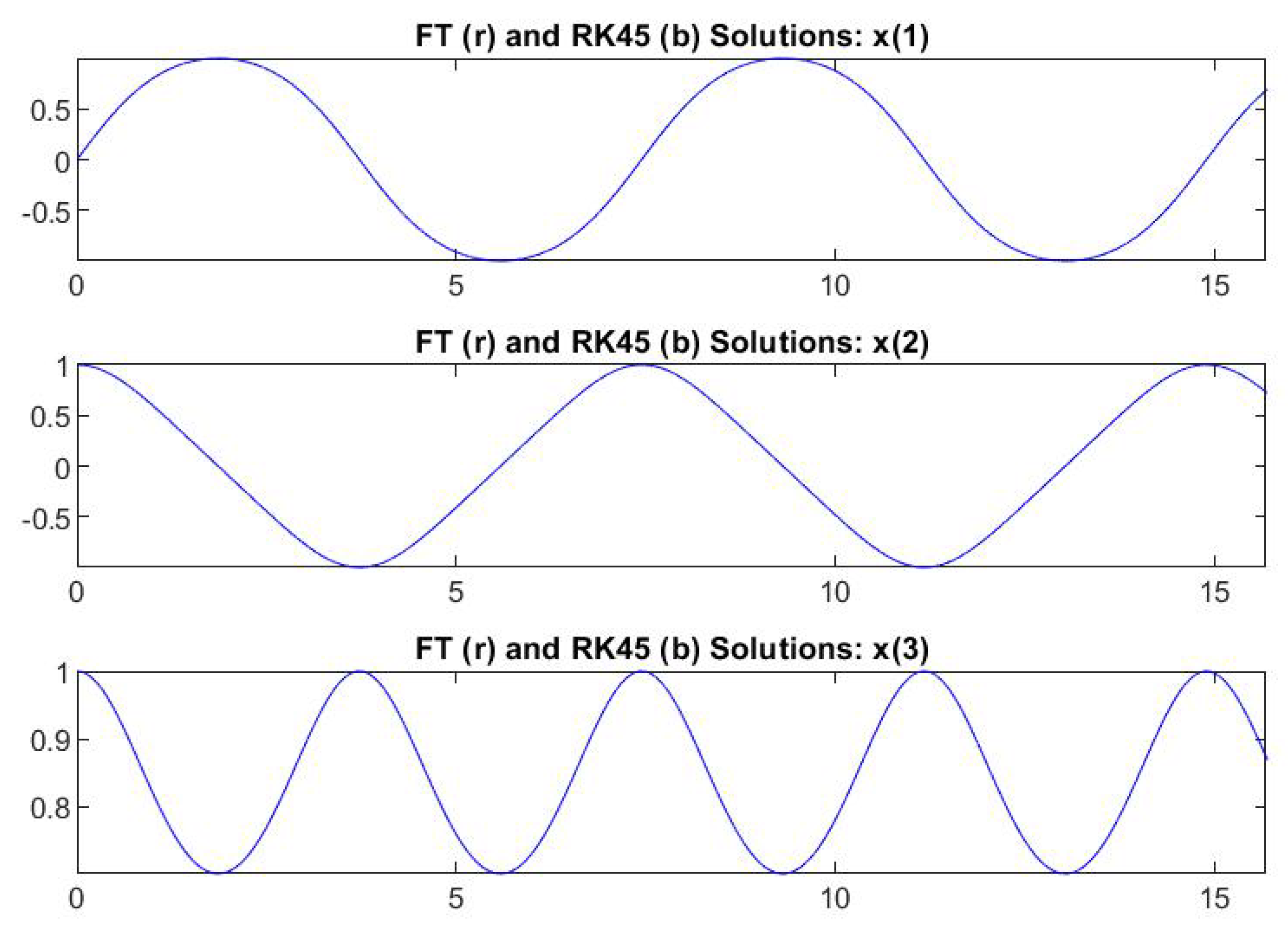
Problem No1: Solution interval is $t\in [0,5\pi ]$;

$$\left\{\begin{array}{cc}{\stackrel{.}{x}}_1=x_2{x}_3\hfill & x_1\left(0\right)=0\hfill \\ {\stackrel{.}{x}}_2=-x_1{x}_3\hfill & x_2\left(0\right)=1\hfill \\ {\stackrel{.}{x}}_3=-0.51x_1{x}_2\hfill & x_3\left(0\right)=1\hfill \end{array}\right.$$

Routine ode45 solves this ODE with optimal step size $h_{ode45}=3.93\times {10}^{-5}$ and final solution vector $x\left(1\right)=6.946876684\times {10}^{-1},x\left(2\right)=7.193115065\times {10}^{-1},x\left(3\right)=8.682618339\times {10}^{-1}.$

We execute ODE-FT with MFT = 10,001, N = 21 so that hstep = 7.853981633974483 $\times {10}^{-5}$, with final solution $x\left(1\right)=6.946876670\times {10}^{-1},x\left(2\right)=7.193115081\times {10}^{-1},x\left(3\right)=8.682618346\times {10}^{-1}.$

At the MFT points $t_i$ where the solution is approximated, the average and the maximum absolute differences between the FT solution and the RK solution for each $x\left(j\right)$ are:

AveDiffFTRK = $1.0\times {10}^{-9}\ast (0.670804140961247,0.565236806318909,0.252472631608888),$

MaxDiffFTRK = $1.0\times {10}^{-8}\ast (0.208394865253148,0.161572011325717,0.078973372286129),$

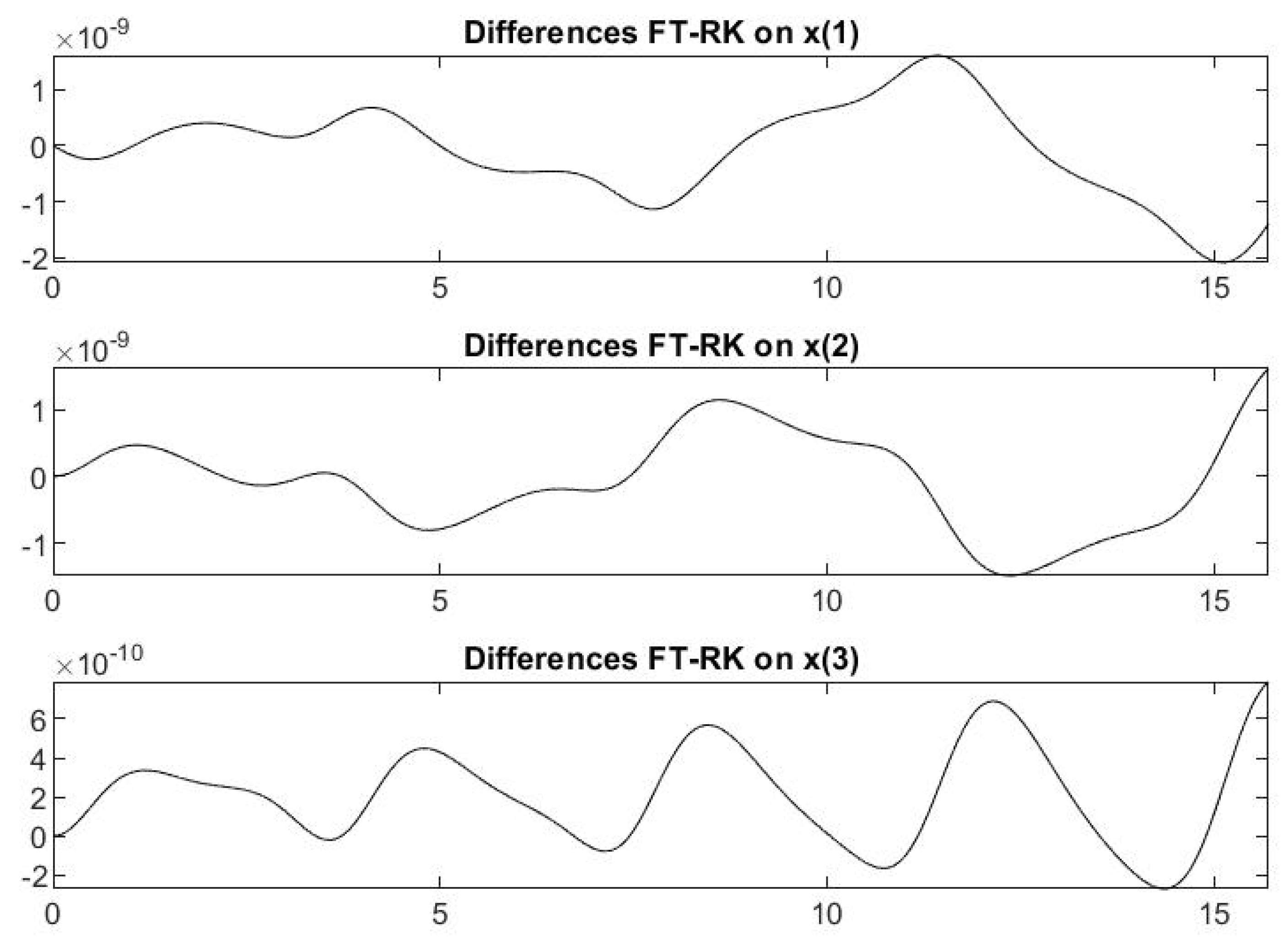
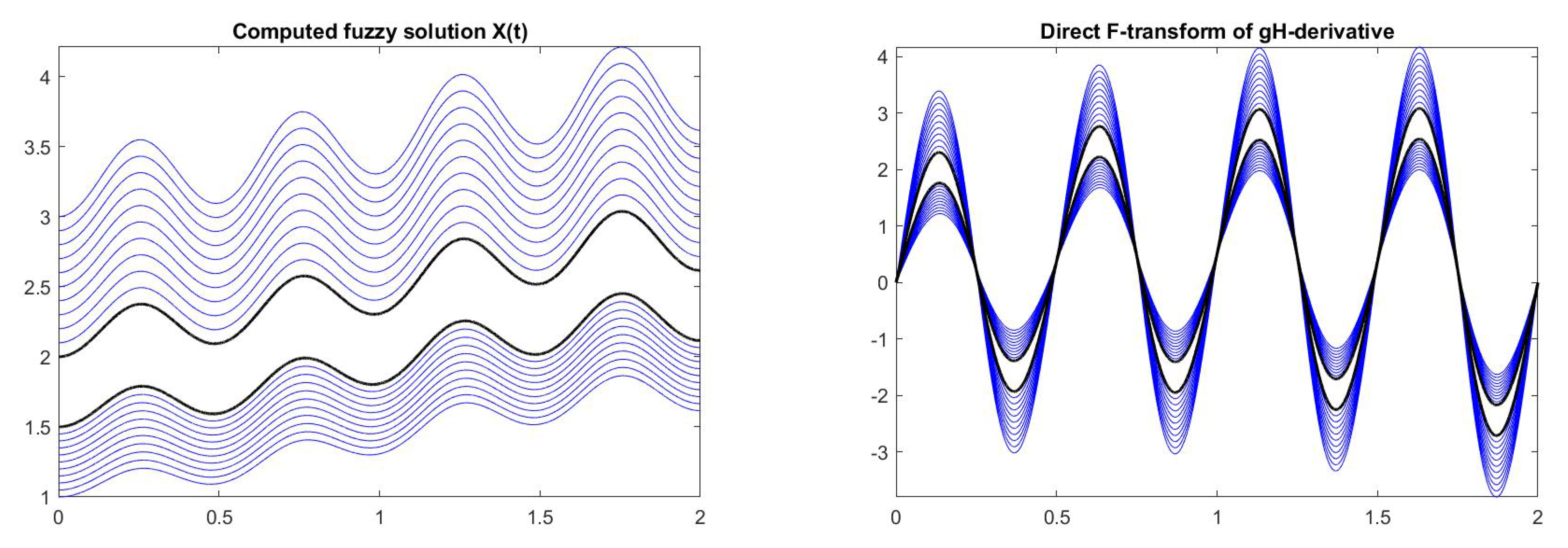
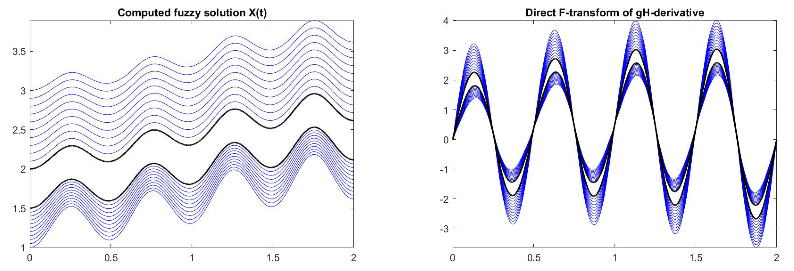
See Figure 1 for the graphical representation of the found solutions. For this example, Figure 2 pictures the differences $FT\left(t\right)-RK\left(t\right)$ between the FT solution and the RK solution for the three components $x_j\left(t\right)$, $j=1,2,3$ at the MFT points. It is interesting to observe that the differences oscillate in sign, showing that in absolute value the differences are not systematically diverging.

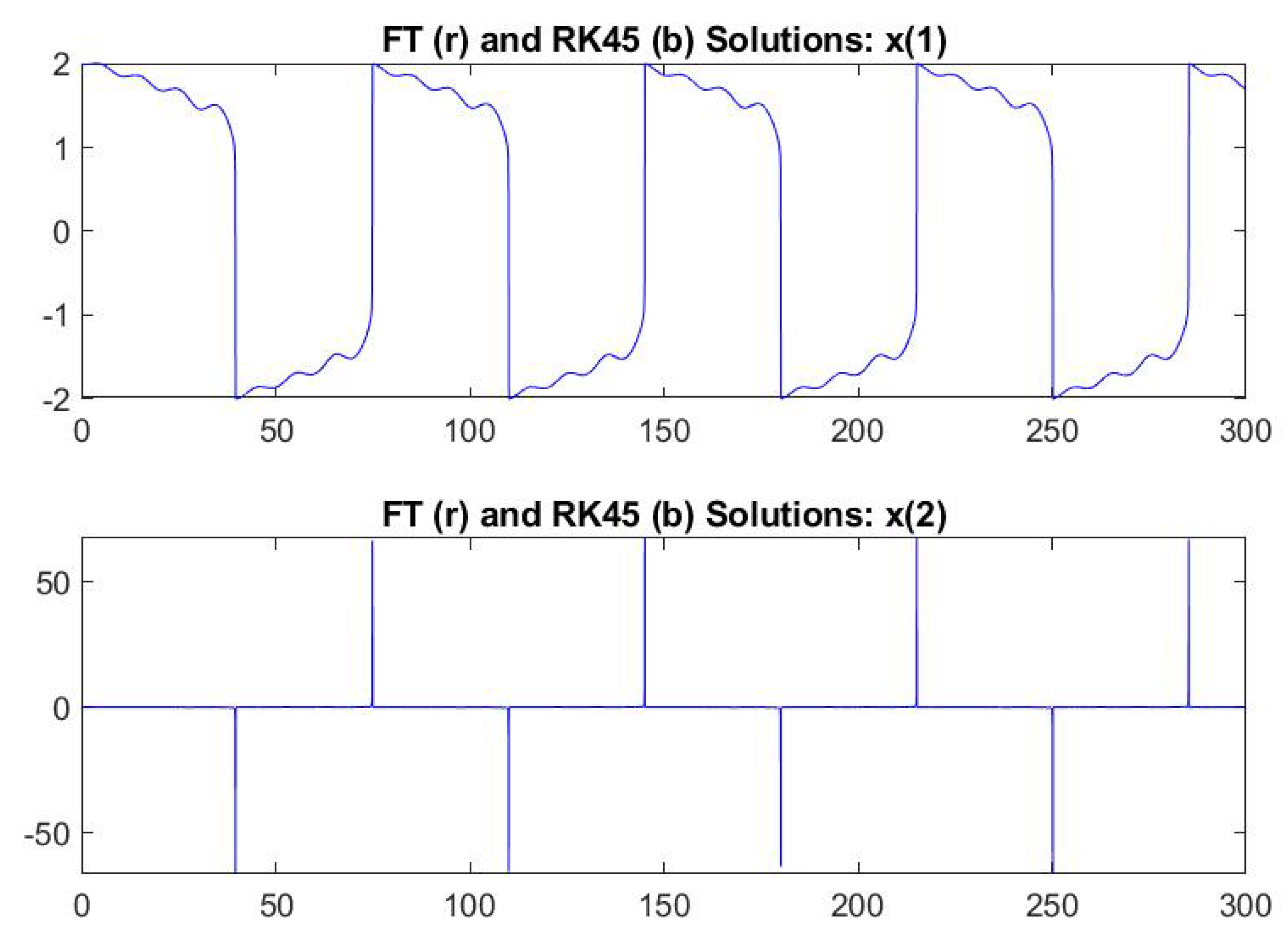
Problem No2: (Van der Pol equations) Solution interval is $t\in [0,300]$;

$$\left\{\begin{array}{c}{\stackrel{.}{x}}_1=x_2\hfill \\ {\stackrel{.}{x}}_2=\mu (1-x_1^2)x_2-x_1+asin\left(\omega t\right)\hfill \\ x_1\left(0\right)=2\hfill \\ x_2\left(0\right)=0.\hfill \end{array}\right.$$

The parameters are $\mu =50$, $a=3$, $\omega =\frac{\pi }{5}$.

This system is considered to be a hard ODE and requires very small step size to determine points where the solution changes suddenly (see Figure 3). To capture this phenomenon, we use M = 30,001. The solution by ode45 has optimal step size $h_{ode45}=2.196\times {10}^{-5}$ and final solution vector $x\left(1\right)=1.700147566\times {10}^0,x\left(2\right)=-1.819270275\times {10}^{-2}$.

With MFT = 30,001, we choose N = 501 to have hstep = 2.0 $\times {10}^{-5}$ and ODE-FT finds the final value $x\left(1\right)=1.700150689\times {10}^0,x\left(2\right)=-1.819263248\times {10}^{-2}$. The comparison gives AveDiffFTRK = 1.398228278980211 $\times {10}^{-4}$ and MaxDiffFTRK = 0.397462807473403.

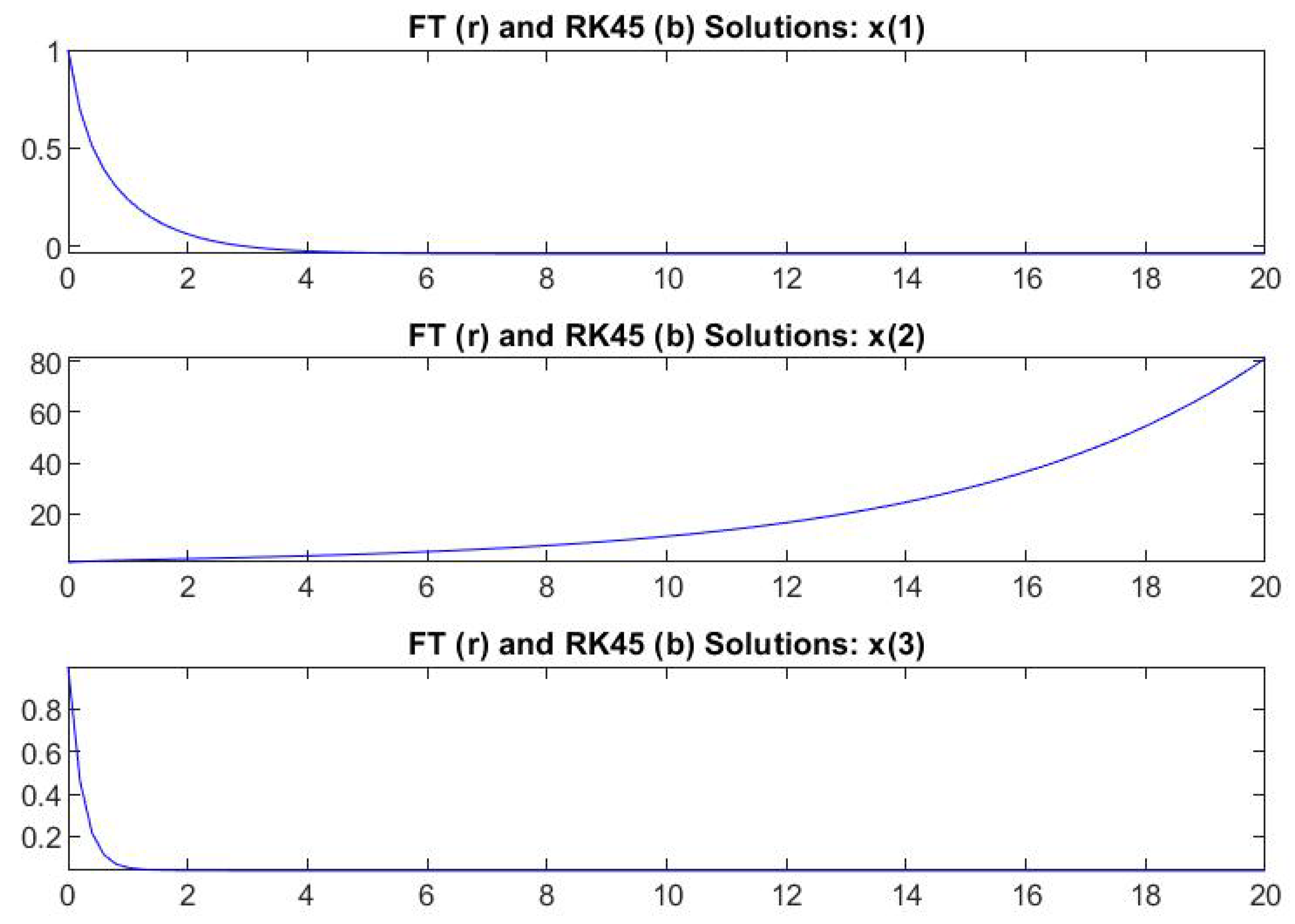
Problem No3: (Rössler’s equations) Solution interval is $t\in [0,20]$;

$$\left\{\begin{array}{cc}{\stackrel{.}{x}}_1=-x_1-x_3\hfill & x_1\left(0\right)=1\hfill \\ {\stackrel{.}{x}}_2=x_1+\alpha x_2\hfill & x_2\left(0\right)=1\hfill \\ {\stackrel{.}{x}}_3=\beta +x_3(x_1-\gamma )\hfill & x_3\left(0\right)=1\hfill \end{array}\right.$$

The parameters are $\alpha =0.2$, $\beta =0.2$, $\gamma =5.0$.

The third equation is nonlinear, but this problem is considered to be not numerically hard. The solution by ode45 has optimal step size $h_{ode45}=0.00144$ and final solution vector $x\left(1\right)=-3.722813228\times {10}^{-1},x\left(2\right)=7.646204266\times {10}^0,x\left(3\right)=3.722813233\times {10}^{-1}.$

With MFT = 101, we choose N = 41 to have hstep = 0.005 and ODE-FT finds the final value $x\left(1\right)=-3.722813228\times {10}^{-1},x\left(2\right)=7.646166172\times {10}^0,x\left(3\right)=3.722813233\times {10}^{-1}.$ The comparison (see Figure 4) gives

AveDiffFTRK = $1.0\times {10}^{-5}\ast (0.025127112474346,0.947056407667963,0.015362751349660),$

MaxDiffFTRK = $1.0\times {10}^{-4}\ast (0.030880110357123,0.380942339370804,0.039961137723310).$

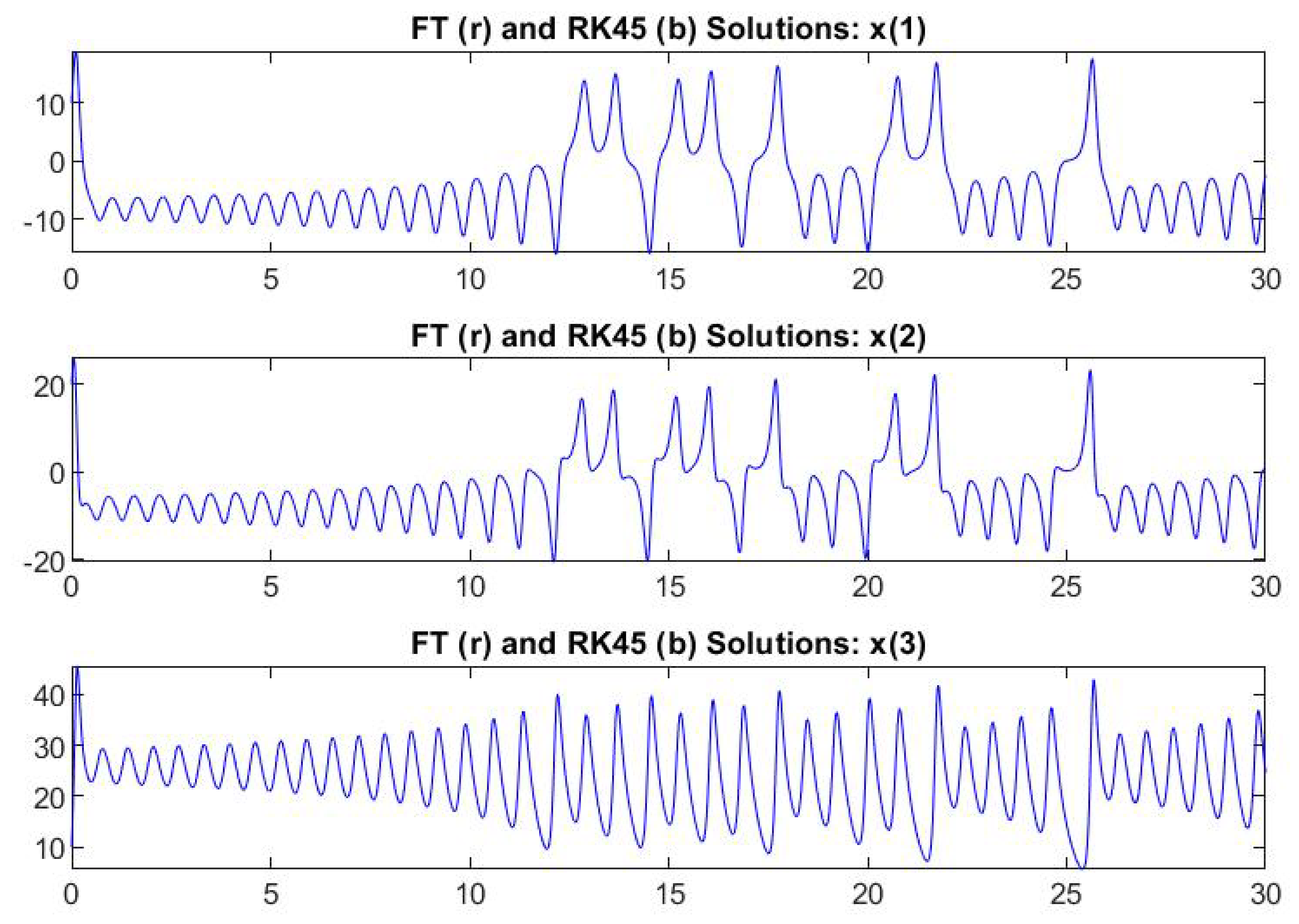
Problem No4: (Lorenz’s system) Solution interval is $t\in [0,100]$;

$$\left\{\begin{array}{cc}{\stackrel{.}{x}}_1=a(x_2-x_1)\hfill & x_1\left(0\right)=10\hfill \\ {\stackrel{.}{x}}_2=x_1(b-x_3)-x_1\hfill & x_2\left(0\right)=20\hfill \\ {\stackrel{.}{x}}_3=x_1{x}_2-c{x}_3\hfill & x_3\left(0\right)=10\hfill \end{array}\right.$$

The parameters are $a=10$, $b=28.0$, $c=\frac{8}{3}$.

It is well known that this nonlinear system is hard to solve numerically as it exhibits chaotic trajectories. Routine ode45 solves the Lorenz system by optimal step size $h_{ode45}=9.37\times {10}^{-7}$ and computes the final value $x\left(1\right)=-2.480991301578959\times {10}^0,x\left(2\right)=4.324784533758371\times {10}^{-1},x\left(3\right)=2.470283374011438\times {10}^1.$ Taking M = 30,001 the step size hstep = 1.0 $\times {10}^{-6}$ is obtained with N = 1001; the found final value using ODE-FT is $x\left(1\right)=-2.453228212514948\times {10}^0,x\left(2\right)=3.798179329138090\times {10}^{-1},x\left(3\right)=2.457087763696305\times {10}^1$ with AveDiffFTRK = (0.004740929429043, 0.006537238822312, 0.008150973471168) and MaxDiffFTRK = (0.149405722393993, 0.285676182819206, 0.328764820957794). 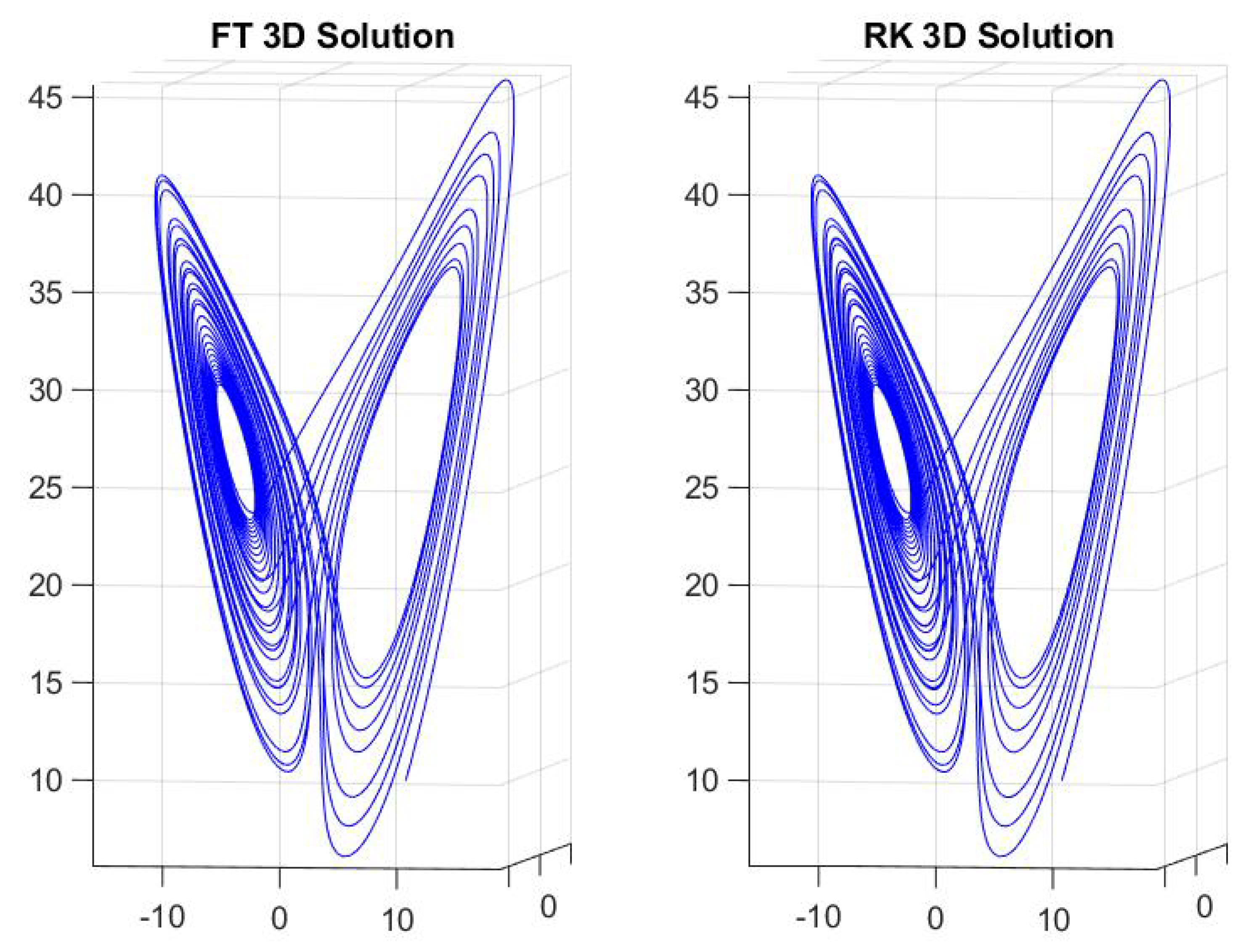See Figure 5 for the trajectories of components $x_j\left(t\right)$, $j=1,2,3$ and Figure 6 for the 3D representations of the solutions.

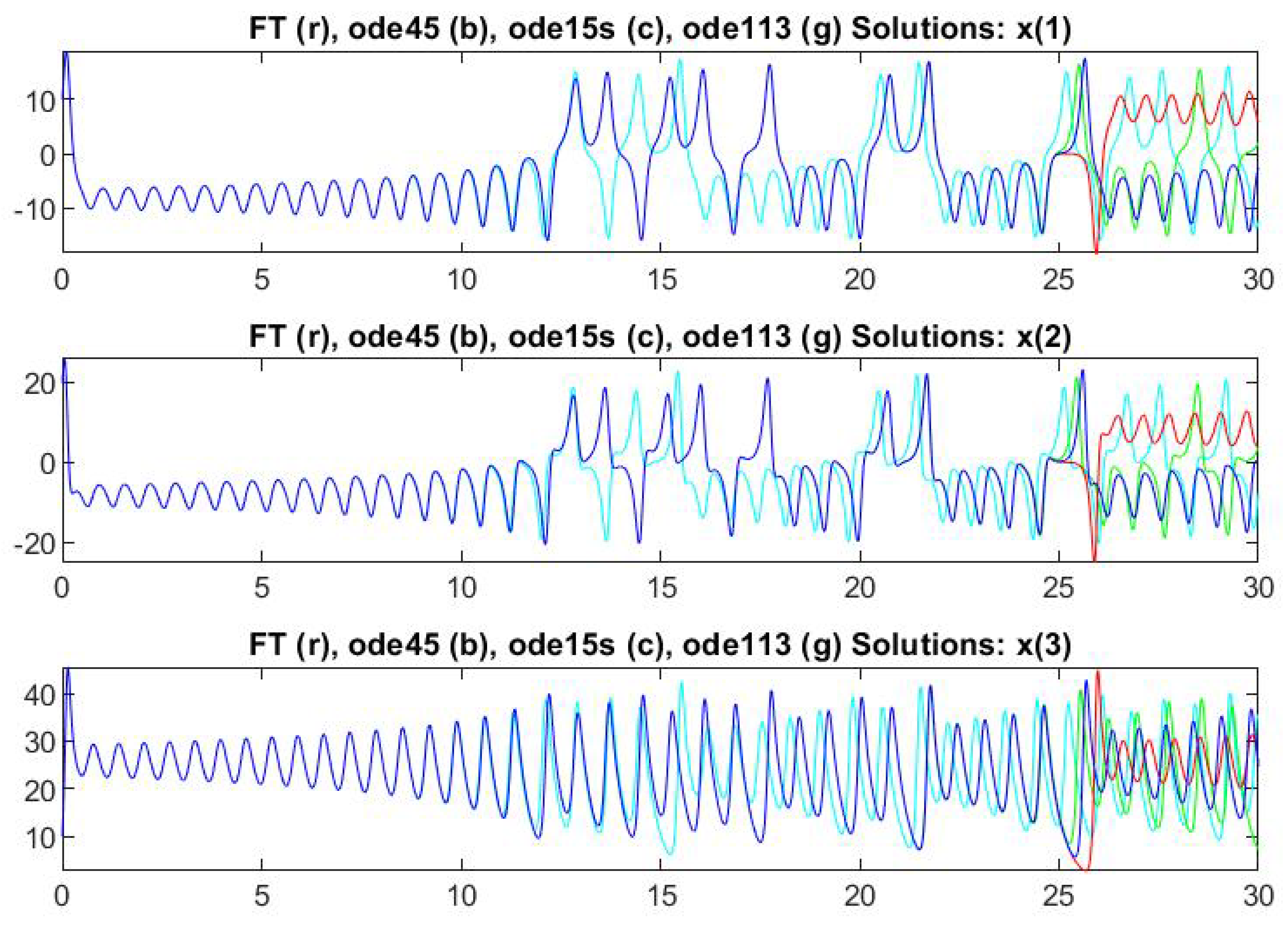
We have also solved this system by a run of ODE-FT with MFT = 30,001, N = 101 and by running the two MATLAB routines ode113 and ode15i; the resulting solutions are visualized in Figure 7 and we see that all the routines tend to generate trajectories with very different behavior for large values of time t.

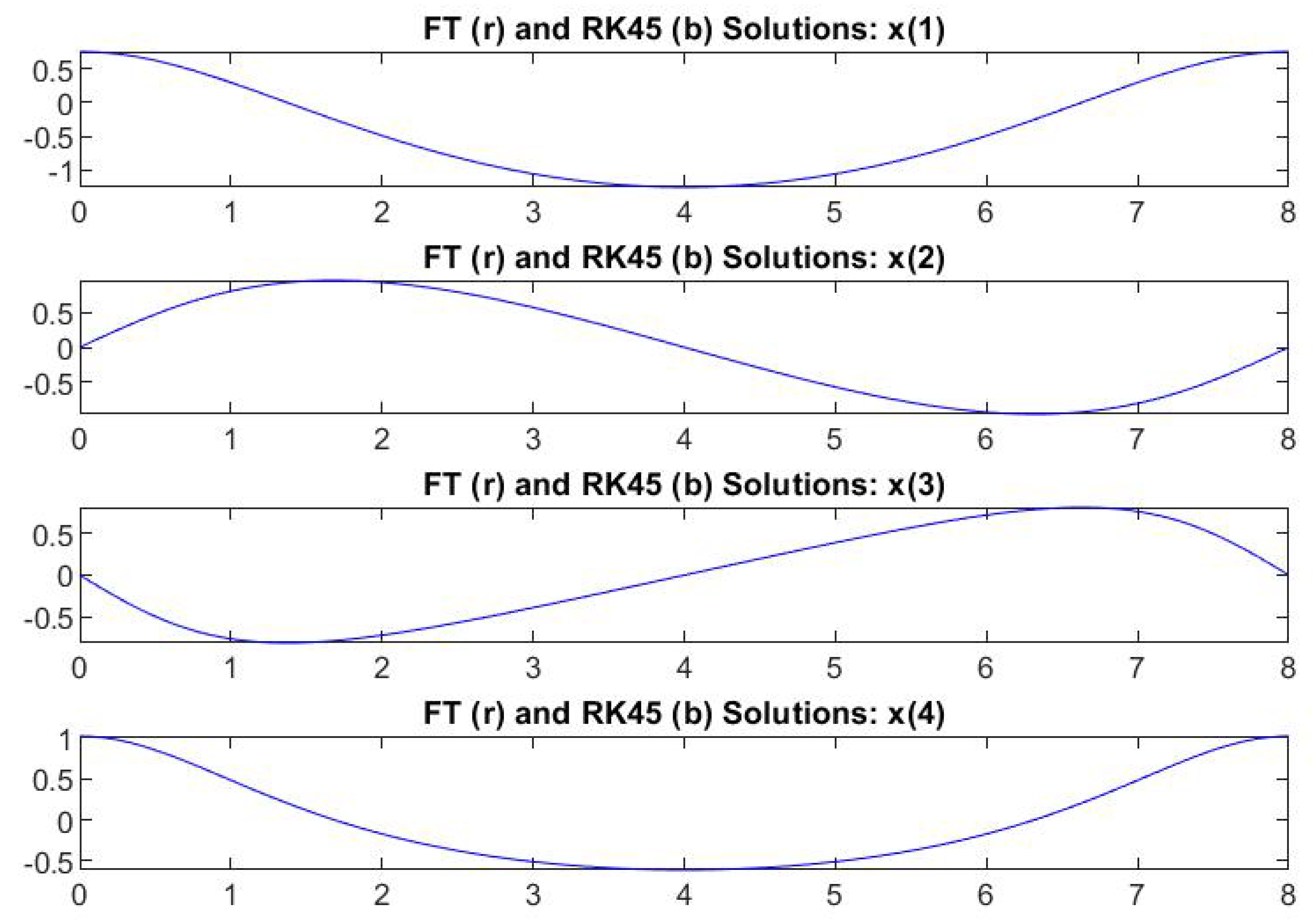
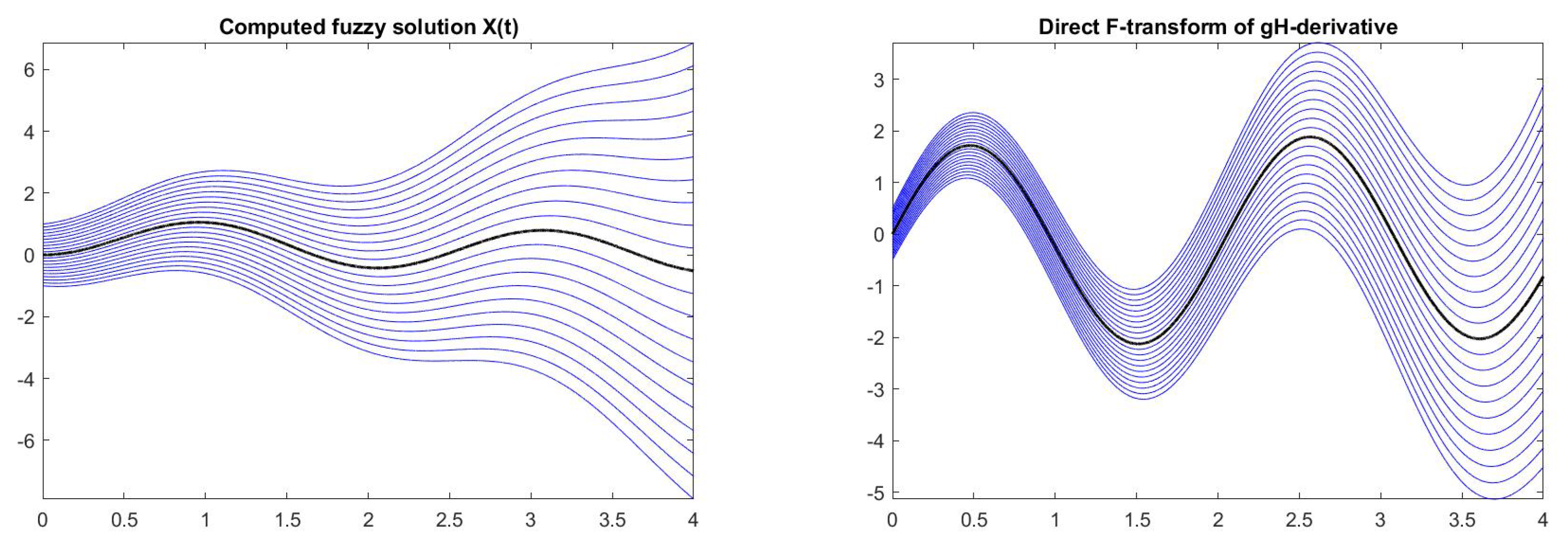
Problem No5: (Periodic system with period $T=8$, see [24], Section 6.8): Solution interval is $t\in [0,8]$;

$$\left\{\begin{array}{cc}{\stackrel{.}{x}}_1=x_3\hfill & x_1\left(0\right)=1-k\hfill \\ {\stackrel{.}{x}}_2=x_4\hfill & x_2\left(0\right)=0\hfill \\ {\stackrel{.}{x}}_3=\frac{-{\alpha }^2{x}_1}{{\left(x_1^2+x_2^2\right)}^{\frac{3}{2}}}\hfill & x_3\left(0\right)=0\hfill \\ {\stackrel{.}{x}}_4=\frac{-{\alpha }^2{x}_2}{{\left(x_1^2+x_2^2\right)}^{\frac{3}{2}}}\hfill & x_4\left(0\right)=\alpha \left(\frac{1+k}{1-k}\right)\hfill \end{array}\right.$$

The parameters are $k=0.25$, $\alpha =\frac{\pi }{4}\sqrt{\frac{1+k}{1-k}}$; we remark that from periodicity, the exact solution has $x_i\left(8\right)=x_i\left(0\right)$, $i=1,\dots ,4$.

The initial condition is $x\left(1\right)=7.50\times {10}^{-1},x\left(2\right)=0.0,x\left(3\right)=0.0,x\left(4\right)=1.013944668993403.$

With MFT = 801, N = 201 and the step size hstep = 5.0 $\times {10}^{-5}$, the final solution found by ODE-FT is $x\left(1\right)=7.500000000000394\times {10}^{-1},x\left(2\right)=-1.890855\times {10}^{-8},x\left(3\right)=1.923939\times {10}^{-8},x\left(4\right)=1.013944668993378$, and the one computed by ode45 is $x\left(1\right)=7.499999999999980\times {10}^{-1},x\left(2\right)=-5.566185\times {10}^{-14},x\left(3\right)=5.123376\times {10}^{-14},x\left(4\right)=1.013944668993403$; comparatively (see Figure 8), we get

AveDiffFTRK = $1.0\times {10}^{-8}\ast (0.4273611,0.3695634,0.3303905,0.3234898),$

MaxDiffFTRK = $1.0\times {10}^{-7}\ast (0.1278607,0.18908499,0.19239342,0.13127243).$

5. Interval (Fuzzy) Differential Equations and F-Transform

In this section, we consider interval and fuzzy differential equations in the setting of generalized Hukuhara differentiability as described in [18,19,25]. A preliminary version of this section has been presented as a conference paper in [17].

Compact intervals of real numbers will be denoted by the usual endpoints notation $A=[a^{-},a^{+}]$, $B=[b^{-},b^{+}]$ or by the midpoint notation $A=(\widehat{a};\tilde{a})$, $B=(\widehat{b};\tilde{b})$ where $\widehat{a}=\frac{1}{2}(a^{-}+a^{+})$ is the midpoint and $\overline{a}=\frac{1}{2}(a^{+}-a^{-})$ is the radius (half-length). The set of all compact real intervals will be denoted by ${\mathcal{K}}_C$.

The use of midpoint representation for intervals has been recently adopted to study several topics in the analysis of interval-valued functions, the single variable case (see [26,27] and the references therein), to which the interested reader is referred for a complete description of interval-valued generalized Hukuhara derivative (gH-derivative for short).

Given two intervals $A,B\in {\mathcal{K}}_C$, the gH-difference is the interval $C\in {\mathcal{K}}_C$ (it always exists and is unique) such that

$$A{⊝}_{gH}B=C⟺\left\{\begin{array}{ccc}\hfill & \left(i\right)\hfill & A=B+C\hfill \\ or\hfill & \left(ii\right)\hfill & B=A-C\hfill \end{array}\right..$$

(33)

Using midpoint notation, we have $A{⊝}_{gH}B=(\widehat{a}-\widehat{b};|\tilde{a}-\tilde{b}|)$ and (i) is verified if $\tilde{a}\ge \tilde{b}$ and $C=(\widehat{a}-\widehat{b};\tilde{a}-\tilde{b})$, (ii) is verified when $\tilde{a}\le \tilde{b}$ and $C=(\widehat{a}-\widehat{b};\tilde{b}-\tilde{a})$. If $\tilde{a}=\tilde{b}$ then clearly $A{⊝}_{gH}B=(\widehat{a}-\widehat{b};0)=\{\widehat{a}-\widehat{b}\}$ is a singleton (real number).

Please note that if $A_i{\ominus }_{gH}{B}_i$ are gH-differences of the same type for all $i=1,\dots ,n$, i.e., all satisfy either (i) or (ii) above, then (see [25])

$${\displaystyle \sum _{i=1}^n}\left(A_i{\ominus }_{gH}{B}_i\right)=\left({\displaystyle \sum _{i=1}^n}{A}_i\right){\ominus }_{gH}\left({\displaystyle \sum _{i=1}^n}{B}_i\right).$$

(34)

An interval-valued function $F:[a,b]\to {\mathcal{K}}_C$ will be denoted by $F\left(t\right)=[f^{-}\left(t\right),f^{+}\left(t\right)]$ or, in equivalent midpoint notation, by $F\left(t\right)=(\widehat{f}\left(t\right);\tilde{f}\left(t\right))$, for $t\in [a,b]$.

We will denote by ${\mathbb{R}}_{\mathcal{F}}$ the set of fuzzy numbers, i.e. normal, fuzzy convex, upper semi-continuous and compactly supported fuzzy sets defined over the real line $\mathbb{R}$. The $\alpha$-level set of u (or simply its $\alpha$-cut) is defined by ${\left[u\right]}_{\alpha }=\{x|x\in \mathbb{R},u\left(x\right)\ge \alpha \}$ and, for $\alpha =0$, it is the closure of the support ${\left[u\right]}_0=cl\{x|x\in \mathbb{R},u\left(x\right)>0\}$.

A well-known result (see [21]) allows us to represent a fuzzy number as a pair $u=\left(u^{-},u^{+}\right)$ of functions $u^{-},u^{+}:\left[0,1\right]⟶\mathbb{R}$, defining the endpoints of the $\alpha$-cuts as ${\left[u\right]}_{\alpha }=[u_{\alpha }^{-},u_{\alpha }^{+}]=({\widehat{u}}_{\alpha };{\tilde{u}}_{\alpha })$

We refer to functions $u_{(.)}^{-}$ and $u_{(.)}^{+}$ as the lower and upper branches of u, respectively; the two functions ${\widehat{u}}_{(.)}$, ${\tilde{u}}_{(.)}$ are the (level-wise) midpoint and radius functions.

Given fuzzy numbers $u,v\in {\mathbb{R}}_{\mathcal{F}},$ the level-wise generalized Hukuhara difference (LgH-difference for short) is the family of intervals

$$u{⊝}_{LgH}v=\left\{{\left[u\right]}_{\alpha }{\ominus }_{gH}{\left[v\right]}_{\alpha }|\alpha \in [0,1]\right\}.$$

A fuzzy-valued function $F:[a,b]\to {\mathbb{R}}_{\mathcal{F}}$ will have $\alpha$-cuts denoted by ${\left[F\left(t\right)\right]}_{\alpha }=[f_{\alpha }^{-}\left(t\right),f_{\alpha }^{+}\left(t\right)]$ or, equivalently, by $({\widehat{f}}_{\alpha }\left(t\right);{\tilde{f}}_{\alpha }\left(t\right))$, for $t\in [a,b]$. Remark that for each $\alpha \in [0,1]$, the functions ${\left[F\right]}_{\alpha }:[a,b]\to {\mathcal{K}}_C$ defined by ${\left[F\right]}_{\alpha }\left(t\right)={\left[F\left(t\right)\right]}_{\alpha }$ are properly interval-valued functions and their family (sometimes called their bunch) $\left\{{\left[F\right]}_{\alpha }|\alpha \in [0,1]\right\}$ gives a unique and equivalent representation of F.

The following definition of generalized derivative can be applied both to interval-valued function or to the level-cuts of a fuzzy-valued function.

Definition 1

([18]). Let $t_0\in ]a,b[$ and h be such that $t_0+h\in ]a,b[$.

-

If $F:[a,b]\to {\mathcal{K}}_C$ is an interval-valued function, its gH-derivative at $t_0$ is defined to be the limit, if it exists,

$$F_{gH}^{\prime }\left(t_0\right)=\underset{h\to 0}{lim}\left(\frac{F(t_0+h){⊝}_{gH}F\left(t_0\right)}{h}\right).$$

(35)

-

If $F:]a,b[\to {\mathbb{R}}_{\mathcal{F}}$ is a fuzzy-valued function, its level-wise gH-derivative (LgH-derivative for short) at $t_0$ is defined to be the family of the gH-derivatives of ${\left[F\right]}_{\alpha }$, if they exist for all $\alpha \in [0,1]$, i.e.,

$$\begin{array}{cc}\hfill F_{LgH}^{\prime }\left(t_0\right)& =\left\{{\left({\left[F\right]}_{\alpha }\right)}_{gH}^{\prime }\left(t_0\right)|\alpha \in [0,1]\right\}where\hfill \end{array}$$

(36)

$$\begin{array}{cc}\hfill {\left({\left[F\right]}_{\alpha }\right)}_{gH}^{\prime }\left(t_0\right)& =\underset{h\to 0}{lim}\frac{1}{h}\left({\left[F(t_0+h)\right]}_{\alpha }{⊝}_{gH}{\left[F\left(t_0\right)\right]}_{\alpha }\right).\hfill \end{array}$$

(37)

For an interval-valued function $F:[a,b]\to {\mathcal{K}}_C$, $F\left(t\right)=[f^{-}\left(t\right),f^{+}\left(t\right)]$, when $f^{-}\left(t\right)$ and $f^{+}\left(t\right)$ are both differentiable, we can distinguish two cases, corresponding to (i) and (ii) of (33) (see [18])

Definition 2.

Let $F:[a,b]⟶{\mathcal{K}}_C$ and $t_0\in ]a,b[$ with $f_{\alpha }\left(t\right)$ and $f_{\alpha }\left(t\right)$ both differentiable at $t_0$. We say that

-

$F$ is (i)-gH-differentiable at $t_0$ if

$$(i.)F_{gH}^{\prime }\left(t_0\right)=\left[{\left(f^{-}\right)}^{\prime }\left(t_0\right),{\left(f^{+}\right)}^{\prime }\left(t_0\right)\right]$$

(38)

-

F is (ii)-gH-differentiable at $t_0$ if

$$(ii.)F_{gH}^{\prime }\left(t_0\right)=[{\left(f^{+}\right)}^{\prime }\left(t_0\right),{\left(f^{-}\right)}^{\prime }\left(t_0\right)].$$

(39)

If $F:]a,b[\to {\mathbb{R}}_{\mathcal{F}}$ is a fuzzy-valued function, we define analogously (i)-LgH and (ii)-LgH differentiability of F, with the additional requirement that (38) (or (39), respectively) are valid for all ${\left[F\right]}_{\alpha }$.

As in [18], we say that a point $t_0\in ]a,b[$ is an l-critical point of F if it is a critical point for the length function $len\left(\left[F\left(t\right)\right]\right)=f^{+}\left(t\right)-f^{-}\left(t\right)$. A point $t_0\in ]a,b[$ is a switching point for the gH-differentiability of F, if in any neighborhood V of $t_0$ there exist points $t_1<t_0<t_2$ such that

type-I switch point): at $t_1$ (38) holds while (39) does not hold and at $t_2$ (39) holds and (38) does not hold, or

type-II switch point): at $t_1$ (39) holds while (38) does not hold and at $t_2$ (38) holds and (39) does not hold.

Analogous definitions can be given level-wise for a fuzzy-valued function.

5.1. Numerical Interval ODE by F-Transform

An interval differential equation (IDE) with initial condition can be written in the form

$$\left\{\begin{array}{c}{\stackrel{·}{x}}_{gH}\left(t\right)=F\left(t,x\left(t\right)\right),t\in \left[t_0,t_1\right]\hfill \\ x\left(t_0\right)=x_0\hfill \end{array}\right.$$

(40)

where $F\left(t,x\left(t\right)\right)=[F^{-}\left(t,x\left(t\right)\right),F^{+}\left(t,x\left(t\right)\right)]$ and $x\left(t\right)=[x^{-}\left(t\right),x^{+}\left(t\right)]$ are intervals for all $t\in \left[t_0,t_1\right]$ and $x_0=[x_0^{-},x_0^{+}]$ is an interval initial value.

The gH-derivative of $x\left(t\right)$ is denoted by

$${\stackrel{·}{x}}_{gH}\left(t\right)=[{\stackrel{·}{x}}_{gH}^{-}\left(t\right),{\stackrel{·}{x}}_{gH}^{+}\left(t\right)].$$

We will approximate ${\stackrel{·}{x}}_{gH}\left(t\right)$ by the iF-transforms of the two functions ${\stackrel{·}{x}}_{gH}^{-}\left(t\right)$ and ${\stackrel{·}{x}}_{gH}^{+}\left(t\right)$ on the same fuzzy partition $\left(\mathbb{P},\mathbb{A}\right)$, i.e.,

$$\begin{array}{cc}\hfill {\left({\stackrel{·}{x}}_{gH}^{-}\right)}_{(\mathbb{P},\mathbb{A})}\left(t\right)& =\sum _{j=1}^n{F}_j^{-}{A}_j\left(t\right)\hfill \end{array}$$

(41)

$$\begin{array}{cc}\hfill {\left({\stackrel{·}{x}}_{gH}^{+}\right)}_{(\mathbb{P},\mathbb{A})}\left(t\right)& =\sum _{j=1}^n{F}_j^{+}{A}_j\left(t\right)\hfill \end{array}$$

(42)

where for $j=1,2,\dots ,n$, using the same notation as in Section 2 with $[a,b]=[t_0,t_1]$, $F_j^{-}$ and $F_j^{+}$ are the direct F-transforms of $\left({\stackrel{·}{x}}_{gH}^{-}\right)$ and $\left({\stackrel{·}{x}}_{gH}^{+}\right)$.

From the monotonicity properties of F-transform (see [4,10] ), we know that $F_j^{-}\le F_j^{+}$ (because ${\stackrel{·}{x}}_{gH}^{-}\left(t\right)\le {\stackrel{·}{x}}_{gH}^{+}\left(t\right)$ for all t) and we can define the intervals $F_j=[F_j^{-},F_j^{+}]$. Consequently, in terms of interval arithmetic operations, we also have the following approximation of the (interval-valued) inverse F-transform ${\left({\stackrel{·}{x}}_{gH}\right)}_{(\mathbb{P},\mathbb{A})}\left(t\right)$ of ${\stackrel{·}{x}}_{gH}$:

$${\left({\stackrel{·}{x}}_{gH}\right)}_{(\mathbb{P},\mathbb{A})}\left(t\right)=\sum _{j=1}^n{F}_j{A}_j\left(t\right).$$

On the other hand, the following function is well defined:

$$H\left(t\right)=\underset{t_0}{\overset{t}{\int }}\left(\sum _{j=1}^n{F}_j{A}_j\left(s\right)ds\right)=\sum _{j=1}^n{F}_j{B}_j\left(t\right),t\in \left[t_0,t_1\right]$$

(43)

and $H\left(t_0\right)=0$ (here 0 stands for the interval $[0,0]$). The interval-valued function $H\left(t\right)$ will play a central role in our method to solve the IDE (40).

For simplicity, define the following interval-valued function

$$\phi \left(t\right)=\sum _{j=1}^n{F}_j{A}_j\left(t\right),t\in [t_0,t_1];$$

(44)

Clearly, $\phi$ is a continuous interval-valued function and, from Theorem 43(i) in [18], the integral function $H\left(t\right)=\underset{t_0}{\overset{t}{\int }}\phi \left(s\right)ds$ is gH-differentiable with

$$H_{gH}^{\prime }\left(t\right)=\phi \left(t\right),H\left(t_0\right)=0.$$

The following property is proved in [17].

Proposition 8.

Consider the function $H\left(t\right)$ in (43) and define the two interval-valued functions $\mathsf{\Phi }\left(t\right)$ and $\mathsf{\Psi }\left(t\right)$ on $\left[t_0,t_1\right]$ by

$$\begin{array}{cc}\hfill \mathsf{\Phi }\left(t\right)& =H\left(t\right){\ominus }_{gH}(-x_0)\hfill \end{array}$$

(45)

$$\begin{array}{cc}\hfill \mathsf{\Psi }\left(t\right)& =H\left(t\right)+x_0.\hfill \end{array}$$

(46)

Then

 (1) 

$\mathsf{\Psi }\left(t\right)$ is gH-differentiable with ${\mathsf{\Psi }}_{gH}^{\prime }\left(t\right)={\sum }_{j=1}^n{F}_j{A}_j\left(t\right)$ and $\mathsf{\Psi }\left(t_0\right)=x_0$.

 (2) 

If all the gH-differences $H\left(t\right){\ominus }_{gH}(-x_0)$ are of the same type for all t, then $\mathsf{\Phi }\left(t\right)$ is gH-differentiable with ${\mathsf{\Phi }}_{gH}^{\prime }\left(t\right)={\sum }_{j=1}^n{F}_j{A}_j\left(t\right)$ and $\mathsf{\Phi }\left(t_0\right)=x_0$.

Consequently, if function $\phi :\left[t_0,t_1\right]⟶{\mathcal{K}}_C$ is generated by a fixed fuzzy partition $\left(\mathbb{P},\mathbb{A}\right)$ as in (44) and $H\left(t\right)={\sum }_{j=1}^n{F}_j{B}_j\left(t\right)$, then we have the following two cases:

(1)

If the intervals $F_j$, $j=1,\dots ,n$ are such that

$$\phi \left(t\right)=F\left(t,H\left(t\right)+x_0\right)\mathrm{for}t\in \left[t_0,t_1\right]$$

then $\mathsf{\Psi }\left(t\right)$ defined on $\left[t_0,t_1\right]$ as in (46) is a solution of (40).

(2)

If the intervals $F_j$, $j=1,\dots ,n$ are such that

$$\phi \left(t\right)=f\left(t,H\left(t\right){\ominus }_{gH}(-x_0)\right)\mathrm{for}t\in \left[t_0,t_1\right]$$

then $\mathsf{\Phi }\left(t\right)$ defined on $\left[t_0,t_1\right]$ as in (45) is a solution of (40), provided that all the gH-differences $H\left(t\right){\ominus }_{gH}(-x_0)$ are of the same type for all $t\in \left[t_0,t_1\right]$.

Remark 2.

From the properties of gH-difference, we have that

$$\begin{array}{cc}\hfill \mathsf{\Psi }\left(t\right){\ominus }_{gH}{x}_0& =H\left(t\right)\hfill \\ \hfill \mathsf{\Phi }\left(t\right){\ominus }_{gH}{x}_0& =\left(H\left(t\right){\ominus }_{gH}(-x_0)\right){\ominus }_{gH}{x}_0.\hfill \end{array}$$

It is interesting to observe that function $\mathsf{\Psi }\left(t\right)$ is (i)-gH-differentiable at all points, while function $\mathsf{\Phi }\left(t\right)$ is (i)-gH-differentiable if the differences $H\left(t\right){\ominus }_{gH}(-x_0)$ are of type (i), i.e., if $H\left(t\right)=\mathsf{\Phi }\left(t\right)-x_0$, and is (ii)-gH-differentiable if the differences $H\left(t\right){\ominus }_{gH}(-x_0)$ are of type (ii), i.e., if $x_0=\mathsf{\Phi }\left(t\right)-H\left(t\right)$. Consequently, solution

$$\mathsf{\Psi }\left(t\right)=[{\mathsf{\Psi }}^{-}\left(t\right),{\mathsf{\Psi }}^{+}\left(t\right)]=(\widehat{\mathsf{\Psi }}\left(t\right);\tilde{\mathsf{\Psi }}\left(t\right))$$

has always increasing length, but the same is not true for solution

$$\mathsf{\Phi }\left(t\right)=[{\mathsf{\Phi }}^{-}\left(t\right),{\mathsf{\Phi }}^{+}\left(t\right)]=(\widehat{\mathsf{\Phi }}\left(t\right);\tilde{\mathsf{\Phi }}\left(t\right))$$

in the case where $\mathsf{\Phi }\left(t\right)$ is (ii)-gH-differentiable.

Finally, let $G_j^{-}$ and $G_j^{+}$ be the $O\left(h^3\right)$ approximations, respectively, of $F_j^{-}$ and $F_j^{+}$ similar to (18)–(19); we can see that the interval-valued iF-transform approximation ${\left({\stackrel{·}{x}}_{gH}\right)}_{(\mathbb{P},\mathbb{A})}\left(t\right)={\sum }_{j=1}^n{G}_j{A}_j\left(t\right)$ of ${\stackrel{·}{x}}_{gH}$ is useful in determining conditions for a switching point.

Indeed, if $p_{k-1}<$$p_k<$$p_{k+1}$ are three adjacent points of $\mathbb{P}$ ($2\le k\le n-1$) and we suppose that no switching point exists internally to the two subintervals $[p_{k-1},p_k]$ and $[p_k,p_{k+1}]$ (i.e., possibly, the switching is exactly at $p_k$) then the solution $x\left(t\right)$ must satisfy

$$\begin{array}{cc}\hfill x\left(p_k\right){\ominus }_{gH}x\left(p_{k-1}\right)& =H_k^L\mathrm{and}x\left(p_{k+1}\right){\ominus }_{gH}x\left(p_k\right)=H_k^R\hfill \end{array}$$

(47)

$$\begin{array}{cc}\hfill \mathrm{where}{H}_k^L& =\underset{p_{k-1}}{\overset{p_k}{\int }}{\stackrel{·}{x}}_{gH}\left(t\right)dt\mathrm{and}{H}_k^R=\underset{p_k}{\overset{p_{k+1}}{\int }}{\stackrel{·}{x}}_{gH}\left(t\right)dt.\hfill \end{array}$$

(48)

On the other hand, we have $H_k^L=F_{k-1}{I}_{k-1}^{+}+F_k{I}_k^{-}$ and $H_k^R=F_k{I}_k^{+}+F_{k+1}{I}_{k+1}^{-}$.

Suppose now that $p_k$ is a switching point for the gH-differentiability of $x\left(t\right)$. We have two cases:

(I): (i)-to-(ii) switch: $x\left(t\right)$ is (i)-gH-differentiable on $]p_{k-1},p_k[$ and is (ii)-gH-differentiable on $]p_k,p_{k+1}[$, i.e., $x\left(p_k\right)=x\left(p_{k-1}\right)+H_k^L$ and $x\left(p_k\right)=x\left(p_{k+1}\right)-H_k^R$ so that $x\left(p_{k+1}\right)=(x\left(p_{k-1}\right)+H_k^L){\ominus }_{gH}(-H_k^R)$, where the difference is of type (i);

(II): (ii)-to-(i) switch: $x\left(t\right)$ is (ii)-gH-differentiable on $]p_{k-1},p_k[$ and is (i)-gH-differentiable on $]p_k,p_{k+1}[$, i.e., $x\left(p_{k-1}\right)=x\left(p_k\right)-H_k^L$ and $x\left(p_{k+1}\right)=x\left(p_k\right)+H_k^R$ so that $x\left(p_{k+1}\right)=\left(x\left(p_{k-1}\right){\ominus }_{gH}(-H_k^L)\right)+H_k^R$, where the difference is of type (i).

Instead, if $p_k$ is not a switching point and $x\left(p_{k+1}\right)=x\left(p_{k-1}\right)+H_k^L+H_k^R$ we have a type (i) solution on $]p_{k-1},p_{k+1}[$; or, if $x\left(p_{k-1}\right)=x\left(p_{k+1}\right)-H_k^L+H_k^R$ we have a type (ii) solution on $]p_{k-1},p_{k+1}[$.

In terms of midpoint notation for intervals, we can summarize the discussion above as follows:

Types of switching points:Let$\left(\mathbb{P},\mathbb{A}\right)$be a fuzzy partition of$\left[t_0,t_1\right]$and$p_{k-1}<$$p_k<$$p_{k+1}$($2\le k\le n-1$); let$x\left(t\right)=(\widehat{x}\left(t\right);\tilde{x}\left(t\right))$be a solution to (40) and$H_k^L=({\widehat{H}}_k^L,{\tilde{H}}_k^L)$and$H_k^R=({\widehat{H}}_k^R,{\tilde{H}}_k^R)$be given as in (48). Then, the midpoint values satisfy

$$\begin{array}{cc}\hfill \widehat{x}\left(p_k\right)& =\widehat{x}\left(p_{k-1}\right)+{\widehat{H}}_k^L\hfill \\ \hfill \widehat{x}\left(p_{k+1}\right)& =\widehat{x}\left(p_{k-1}\right)+{\widehat{H}}_k^L+{\widehat{H}}_k^R.\hfill \end{array}$$

Assuming that only$p_k$ is eventually a switching point, we have the following four cases

 (a) 

if$p_k$is a (i)-to-(ii) switch, then

$$\begin{array}{cc}\hfill \tilde{x}\left(p_k\right)& =\tilde{x}\left(p_{k-1}\right)+{\tilde{H}}_k^L\hfill \\ \hfill \tilde{x}\left(p_{k+1}\right)& =\tilde{x}\left(p_{k-1}\right)+{\tilde{H}}_k^L-{\tilde{H}}_k^R\ge 0\hfill \end{array}$$

 (b) 

if$p_k$is a (ii)-to-(i) switch, then

$$\begin{array}{cc}\hfill \tilde{x}\left(p_k\right)& =\tilde{x}\left(p_{k-1}\right)-{\tilde{H}}_k^L\ge 0\hfill \\ \hfill \tilde{x}\left(p_{k+1}\right)& =\tilde{x}\left(p_{k-1}\right)-{\tilde{H}}_k^L+{\tilde{H}}_k^R\ge 0\hfill \end{array}$$

 (c) 

if$x\left(t\right)$is (i)-gH- differentiable on$[p_{k-1},p_{k+1}]$, then

$$\begin{array}{cc}\hfill \tilde{x}\left(p_k\right)& =\tilde{x}\left(p_{k-1}\right)+{\tilde{H}}_k^L\hfill \\ \hfill \tilde{x}\left(p_{k+1}\right)& =\tilde{x}\left(p_{k-1}\right)+{\tilde{H}}_k^L+{\tilde{H}}_k^R\hfill \end{array}$$

 (d) 

if$x\left(t\right)$is (ii)-gH- differentiable on$[p_{k-1},p_{k+1}]$, then

$$\begin{array}{cc}\hfill \tilde{x}\left(p_k\right)& =\tilde{x}\left(p_{k-1}\right)-{\tilde{H}}_k^L\ge 0\hfill \\ \hfill \tilde{x}\left(p_{k+1}\right)& =\tilde{x}\left(p_{k-1}\right)-({\tilde{H}}_k^L+{\tilde{H}}_k^R)\ge 0.\hfill \end{array}$$

There are no general rules to locate a switching point. Denote by $x\left(t\right)=$ $[x^{-}\left(t\right),x^{+}\left(t\right)]=$$(\widehat{x}\left(t\right);\tilde{x}\left(t\right))$ a solution of the IDE (40); if $x\left(t\right)$ is (i)-gH-differentiable, its length $\tilde{x}\left(t\right)$ will not decrease, while $\tilde{x}\left(t\right)$ will not increase if $x\left(t\right)$ is (ii)-gH-differentiable. Some authors have noticed that possibly, the sequence of switching points can be pre-defined a priori, by positioning them in the time domain of the interval differential equation; this is true, at least in principle, provided that the found solution is guaranteed to have exactly them and not other switching points, but such purely exogenous proposal is not fully convincing.

An endogenous way may be preferred, similar to control strategies, to connect the type of gH-differentiability to the evolution of the trajectory. For example, it seems reasonable to locate the switching points depending on how the solution is evolving, by fixing a lower $l\left(t\right)$ and an upper threshold $u\left(t\right)$, say $0\le L\le l\left(t\right)\le u\left(t\right)\le U$ and requiring that $l\left(t\right)\le \tilde{x}\left(t\right)\le u\left(t\right)$ for all t; then,

(a)

a (i)-to-(ii) switch is decided at $t=p_k$ if the following condition is reached

$$\left\{\begin{array}{c}\tilde{x}\left(p_k\right)=\tilde{x}\left(p_{k-1}\right)+{\tilde{H}}_k^L\le u\left(p_k\right)\hfill \\ \tilde{x}\left(p_{k+1}\right)=\tilde{x}\left(p_{k-1}\right)+{\tilde{H}}_k^L+{\tilde{H}}_k^R>u\left(p_{k+1}\right)\hfill \end{array}\right.$$

(b)

a (ii)-to-(i) switch is decided at $t=p_k$ if the following condition is reached

$$\left\{\begin{array}{c}\tilde{x}\left(p_k\right)=\tilde{x}\left(p_{k-1}\right)-{\tilde{H}}_k^L\ge l\left(p_k\right)\hfill \\ \tilde{x}\left(p_{k+1}\right)=\tilde{x}\left(p_{k-1}\right)-{\tilde{H}}_k^L-{\tilde{H}}_k^R<l\left(p_{k+1}\right).\hfill \end{array}\right.$$

In some sense, the rule above will control the increasing and decreasing of “uncertainty” in an endogenous way, without any reference to the interval initial condition $x_0$ or to the interval-valued function $F(t,x)$.

Furthermore, we are essentially free to decide the type of differentiability at the initial point; if the initial length ${\tilde{x}}_0$ is such that $L<{\tilde{x}}_0<U$, we can start either with a type c) or a type d) and a unique solution is then found by applying the decided switching rule.

A different purely endogenous rule can be obtained by following the increase or decrease of $\tilde{x}\left(t\right)$ and trying to intercept points $t^{\ast }$ where the function $\tilde{x}\left(t\right)$ has a local maximum (for a (i)-to-(ii) switch) or a local minimum (for a (ii)-to-(i) switch). A necessary condition can be obtained according to the following simple result:

Endogenous criteria for a switching point:Assume that$x\left(t\right)=$$[x^{-}\left(t\right),x^{+}\left(t\right)]=$$(\widehat{x}\left(t\right);\tilde{x}\left(t\right))$is such that$x^{-}\left(t\right)$and$x^{+}\left(t\right)$are differentiable so that its gH-derivative${\stackrel{·}{x}}_{gH}\left(t\right)$can be expressed in terms of the derivatives${\left(x^{-}\right)}^{\prime }\left(t\right)$and${\left(x^{+}\right)}^{\prime }\left(t\right)$. Let$(\mathbb{P},\mathbb{A})$be a fuzzy partition of$[t_0,t_1]$and let${\left({\stackrel{·}{x}}_{gH}\right)}_{(\mathbb{P},\mathbb{A})}\left(t\right)={\sum }_{k=1}^n{F}_k{A}_k\left(t\right)$be the iF-transform of${\stackrel{·}{x}}_{gH}\left(t\right)$with interval-valued components$F_k=({\widehat{F}}_k;{\tilde{F}}_k)$. If$p_k$is a local minimum or maximum of$\tilde{x}\left(t\right)$, then${\tilde{F}}_k=0+O\left(h^2\right)$.

Proof. 

From the properties of F-transform, we have $F_k^{-}={\left({\stackrel{·}{x}}_{gH}\right)}^{-}\left(p_k\right)+O\left(h^2\right)$, $F_k^{+}={\left({\stackrel{·}{x}}_{gH}\right)}^{+}\left(p_k\right)+O\left(h^2\right)$ and, in particular, ${\tilde{F}}_k=$ $\widetilde{{\stackrel{·}{x}}_{gH}}\left(p_k\right)+O\left(h^2\right)$. On the other hand, from the differentiability of $x^{-}\left(t\right)$ and $x^{+}\left(t\right)$, we have $0=\frac{d}{dt}\tilde{x}\left(t\right))$ for $t=p_k$, i.e., ${\left(x^{+}\right)}^{\prime }\left(p_k\right)-{\left(x^{-}\right)}^{\prime }\left(p_k\right)=0$. It follows that $\widetilde{{\stackrel{·}{x}}_{gH}}\left(p_k\right)=\left|\frac{{\left(x^{+}\right)}^{\prime }\left(p_k\right)-{\left(x^{-}\right)}^{\prime }\left(p_k\right)}{2}\right|=0$, i.e., ${\tilde{F}}_k=$$\widetilde{{\stackrel{·}{x}}_{gH}}\left(p_k\right)+O\left(h^2\right)=$$0+O\left(h^2\right)$.  □

We then suggest the following (purely endogenous) switching rule.

Switching rule for IDE: Let $(\mathbb{P},\mathbb{A})$ be a fuzzy partition of $[t_0,t_1]$ and suppose we have computed the approximate solution $x\left(p_i\right)$ of IDE (40) at the points $t_0=p_1<p_2<\dots <p_k$ with $k<n$. Assume that $h=\frac{t_1-t_0}{n-1}$ is sufficiently small and $p_i=p_{i-1}+h$.

In any case, the midpoint value is computed as $\widehat{x}\left(p_k\right)=\widehat{x}\left(p_{k-1}\right)+{\widehat{F}}_{k-1}{I}_{k-1}^{+}+{\widehat{F}}_k{I}_k^{-}$.

(1)

If $x\left(p_k\right)$ is computed according to (i)-gH-differentiability on $[p_{k-1},p_k]$, i.e., $\tilde{x}\left(p_k\right)=\tilde{x}\left(p_{k-1}\right)+{\tilde{F}}_{k-1}{I}_{k-1}^{+}+{\tilde{F}}_k{I}_k^{-}$ and if ${\tilde{F}}_k=O\left(h^2\right)$, then $p_k$ is assumed to be a (i)-to-(ii) switch and the next iteration is performed according to (ii)-gH-differentiability.

(2)

If $x\left(p_k\right)$ is computed according to (ii)-gH-differentiability on $[p_{k-1},p_k]$, i.e., $\tilde{x}\left(p_k\right)=\tilde{x}\left(p_{k-1}\right)-{\tilde{F}}_{k-1}{I}_{k-1}^{+}-{\tilde{F}}_k{I}_k^{-}$ and if ${\tilde{F}}_k=O\left(h^2\right)$, then $p_k$ is assumed to be a (ii)-to-(i) switch and the next iteration is performed according to (i)-gH-differentiability.

In our computations, the test ${\tilde{F}}_k=O\left(h^2\right)$ is performed by the condition ${\tilde{F}}_k<\epsilon$ for a small tolerance $\epsilon >0$ (say $\epsilon \in [{10}^{-3},{10}^{-5}]$).

5.2. Numerical Procedure for IDE

We are now ready to summarize the proposed procedure to solve the IDE (40) on $[t_0,t_1]$, based on F-transform of the gH-derivative ${\stackrel{·}{x}}_{gH}\left(t\right)$.

Chose a uniform fuzzy partition $\left(\mathbb{P},\mathbb{A}\right)$ with $n>2$ points $\mathbb{P}=\left\{t_0=p_1<\dots <p_n=t_1\right\}$ and basic functions $\mathbb{A}=\left\{A_1,\dots ,A_n\right\}$.

From the properties of the F-transforms on $\left({\mathbb{P}}_k,{\mathbb{A}}_k\right)$, we have

$${\int }_{p_1}^{p_k}{\stackrel{·}{x}}_{gH}\left(t\right)dt=\sum _{j=1}^{k-1}{\int }_{p_1}^{p_k}{F}_j{A}_j\left(t\right)dt+{\int }_{p_1}^{p_k}{\tilde{F}}_k{\tilde{A}}_k\left(t\right)dt$$

for all $k=2,\dots ,n$, where

$${\tilde{F}}_k=\frac{{\int }_{p_{k-1}}^{p_k}{\stackrel{·}{x}}_{gH}\left(t\right)A_k\left(t\right)dt}{{\int }_{p_{k-1}}^{p_k}{A}_k\left(t\right)dt}.$$

With the introduced notation, we solve (40) by the following procedure, assuming that no switching point exists on $\left[p_{k-1},p_k\right]$ and $x_0$ is the given initial condition.

Algorithm IDE-FT: Find an approximated final value $x_{(\mathbb{P},\mathbb{A})}\left(t_1\right)$ of the IDE ${\stackrel{·}{x}}_{gH}\left(t\right)=F\left(t,x\left(t\right)\right),$$t\in \left[t_0,t_1\right]$ with initial condition $x\left(t_0\right)=x_0.$

Step 1.

Chose one of the two models (45) or (46) to start with, say $Meth=1$ for (i)-gH-differentiability (increasing length) and $Meth=2$ for (ii)-gH-differentiability (decreasing length); chose a positive tolerance $\epsilon >0$ to test for switching; chose $n>2$, set $h=\frac{t_1-t_0}{n-1}$ so that $p_j=t_0+(j-1)h$ for $j=1,\dots ,n$ and chose a family $\mathbb{A}$ of basic functions.

Step 2.

Compute $F_1=f\left(t_0,x_0\right)$. Set $H=F_1{I}_1^{+}$, $y=x_0$.

Step 3.

For $k=2,3,\dots ,n$, the interval-valued components ${\tilde{F}}_k$, $F_k$ are first approximated iteratively by finding ${\tilde{F}}_k$ as a fixed point

$${\tilde{F}}_k=\frac{h}{I_k^{-}}f\left(p_k,y+H+{\tilde{F}}_k{I}_k^{-}\right)\mathrm{if}Meth=1$$

or

$${\tilde{F}}_k=\frac{h}{I_k^{-}}f\left(p_k,\left(y+H+{\tilde{F}}_k{I}_k^{-}\right){\ominus }_{gH}(-x_0)\right)\mathrm{if}Meth=2$$

and $F_k=2I_k^{-}{\tilde{F}}_k/I_k$. Set the new solution interval value for $t=p_k$ as

$$x\left(p_k\right)=\left\{\begin{array}{ccc}y+H+F_k{I}_k^{-}& \mathrm{if}& Meth=1\\ \left(H+F_k{I}_k^{-}\right){\ominus }_{gH}(-y)& \mathrm{if}& Meth=2\end{array}\right.$$

Step 4.

(Test for a switching at $p_k$) If ${\tilde{F}}_k<\epsilon$, then $p_k$ is declared to be a switch of gH-differentiability: if so, exchange the value of $Meth$ from 1 to 2 or from 2 to 1; set $H=f(p_k,x\left(p_k\right))I_k^{+}$, $y=x\left(p_k\right)$. If instead ${\tilde{F}}_k>\epsilon$, then $p_k$ is not a switch: in this case, update H to $H+F_k{I}_k^{-}$, without changing $Meth$.

Step 5.

Continue from step 3 with next k, until the final point $t_1$ is reached.

5.3. Application to Fuzzy Differential Equations

If the fuzzy-valued function $\phi :[a,b]⟶{\mathbb{R}}_{\mathcal{F}}$ is gH-differentiable with respect to t, or if it is level-wise gH-differentiable, we can approximate its gH-derivative ${\phi }_{gH}^{\prime }$ or its LgH-derivative ${\phi }_{LgH}^{\prime }$ by a family of interval-valued iF-transforms, parametrized with $\alpha \in [0,1]$, in terms of its $\alpha$-cuts (consider that $A_j\left(x\right)\ge 0$ for all x and all j)

$$\begin{array}{cc}\hfill {\left({\left[{\phi }_{gH}^{\prime }\left(x\right)\right]}_{\alpha }\right)}_{(P,A)}={\displaystyle \sum _{j=1}^n}{F}_{j,\alpha }{A}_j\left(x\right)& =\left[{\displaystyle \sum _{j=1}^n}{F}_{j,\alpha }^{-}{A}_j\left(x\right),{\displaystyle \sum _{j=1}^n}{F}_{j,\alpha }^{+}{A}_j\left(x\right)\right].\hfill \end{array}$$

The F-transform of ${\phi }_{gH}^{\prime }$ is then obtained by the family of F-transforms of the lower and upper functions ${\left({\phi }_{gH}^{\prime }\right)}_{j,\alpha }^{-}\left(x\right)$ and ${\left({\phi }_{gH}^{\prime }\right)}_{j,\alpha }^{+}\left(x\right)$:

$$\begin{array}{cc}\hfill F_{j,\alpha }^{-}& =\frac{\underset{a}{\overset{b}{\int }}{\left({\phi }_{gH}^{\prime }\right)}_{j,\alpha }^{-}\left(x\right)A_j\left(x\right)dx}{\underset{a}{\overset{b}{\int }}{A}_j\left(x\right)dx},j=1,2,\dots ,n\hfill \\ \hfill F_{j,\alpha }^{+}& =\frac{\underset{a}{\overset{b}{\int }}{\left({\phi }_{gH}^{\prime }\right)}_{j,\alpha }^{+}\left(x\right)A_j\left(x\right)dx}{\underset{a}{\overset{b}{\int }}{A}_j\left(x\right)dx},j=1,2,\dots ,n.\hfill \end{array}$$

and, considering that each $A_j$ is a continuous non-negative function, we can obtain an approximation of $\phi \left(x\right)$ by

$$\begin{array}{c}\hfill \phi \left(x\right){⊝}_{gH}\phi \left(a\right)=\underset{a}{\overset{x}{\int }}{\phi }_{gH}^{\prime }\left(t\right)dt={\displaystyle \sum _{j=1}^n}\left({\phi }_{gH}^{\prime }\left(x_j\right)\underset{a}{\overset{x}{\int }}{A}_j\left(t\right)dt\right).\end{array}$$

Consider now an FDE in gH-derivative form

$$\begin{array}{cc}\hfill {\phi }_{gH}^{\prime }\left(x\right)& =f(x,\phi \left(x\right))\mathrm{for}x\in [x_1,x_q]\hfill \\ \hfill \phi \left(x_1\right)& ={\phi }_1;\hfill \end{array}$$

we approximate ${\phi }_{gH}^{\prime }\left(x\right)={\displaystyle \sum _{j=1}^q}{\phi }_{gH}^{\prime }\left(x_j\right)B_j\left(x\right)$ and substituting the condition ${\phi }_{gH}^{\prime }\left(x\right)=f(x,\phi \left(x\right))$ into the approximation, we obtain

$${\phi }_{gH}^{\prime }\left(x\right)={\displaystyle \sum _{j=1}^q}f(x,\phi \left(x\right))A_j\left(x\right);$$

Integrating with given initial condition $\phi \left(x_1\right)={\phi }_1$ we obtain

$$\phi \left(x\right){⊝}_{gH}{\phi }_1=\underset{x_1}{\overset{x}{\int }}f(t,\phi \left(t\right))dt$$

and, at the points $x_j\in \mathbb{P}$, defining ${\phi }_j=\phi \left(x_j\right)$, $j=2,\dots ,q$,

$$\begin{array}{cc}\hfill {\phi }_2{⊝}_{gH}{\phi }_1& =f(x_1,{\phi }_1)I_1^{+}+f(x_2,{\phi }_2)I_2^{-}\hfill \\ \hfill \mathrm{and},\mathrm{for}j& =3,\dots ,n\hfill \\ \hfill {\phi }_j{⊝}_{gH}{\phi }_1& ={\displaystyle \sum _{l=1}^{j-1}}f(x_l,{\phi }_l)(I_l^{-}+I_l^{+})+f(x_j,\phi \left(x_j\right))I_j^{-}.\hfill \end{array}$$

These are (generally nonlinear) non-differential fuzzy equations of the form

$${\phi }_j{⊝}_{gH}{\phi }_1=c_{j-1}+f(x_j,{\phi }_j)I_j^{-},j=2,3,\dots ,n$$

where when solving for ${\phi }_j$, the fuzzy numbers ${\phi }_1,{\phi }_2,\dots ,{\phi }_{j-1}$ are determined in previous steps and the fuzzy quantity

$$c_{j-1}={\displaystyle \sum _{l=1}^{j-1}}f(x_l,{\phi }_l)(I_l^{-}+I_l^{+})$$

is known.

If we search for a (i)-gH-differentiable solution, the fuzzy equation for ${\phi }_j$ is

$${\phi }_j={\phi }_1+c_{j-1}+f(x_j,{\phi }_j)I_j^{-};$$

if we search for a (ii)-gH-differentiable solution, the fuzzy equation for ${\phi }_j$ is

$${\phi }_1={\phi }_j+(-c_{j-1}-f(x_j,{\phi }_j)I_j^{-}).$$

In terms of $\alpha$-cuts, they can be written (for $\alpha \in [0,1]$ or $\alpha \in \{{\alpha }_1,{\alpha }_2,\dots ,{\alpha }_p\}$)

$$\begin{array}{cc}\hfill {\phi }_{j,\alpha }^{-}& ={\phi }_{1,\alpha }^{-}+c_{j-1,\alpha }^{-}+f_{\alpha }^{-}(x_j,{\phi }_{j,\alpha }^{-},{\phi }_{j,\alpha }^{+})I_j^{-}\hfill \\ \hfill {\phi }_{j,\alpha }^{+}& ={\phi }_{1,\alpha }^{+}+c_{j-1,\alpha }^{+}+f_{\alpha }^{+}(x_j,{\phi }_{j,\alpha }^{-},{\phi }_{j,\alpha }^{+})I_j^{-}\hfill \end{array}$$

and

$$\begin{array}{cc}\hfill {\phi }_{1,\alpha }^{-}& ={\phi }_{j,\alpha }^{-}+(-c_{j-1,\alpha }^{+}-f_{\alpha }^{+}(x_j,{\phi }_{j,\alpha }^{-},{\phi }_{j,\alpha }^{+})I_j^{-})\hfill \\ \hfill {\phi }_{1,\alpha }^{+}& ={\phi }_{j,\alpha }^{+}+(-c_{j-1,\alpha }^{-}-f_{\alpha }^{-}(x_j,{\phi }_{j,\alpha }^{-},{\phi }_{j,\alpha }^{+})I_j^{-})\hfill \end{array}$$

respectively.

6. Computational Results for Interval and Fuzzy Differential Equations

For all problems we use $M=10,001$ as the number of points $t_i$ where the solution is computed and $n=11$ as the number of nodes in the partition $(\mathbb{P},\mathbb{A})$; it results that the step size of the method to solve the differential equation on $[a,b]]$ is $h={\displaystyle \frac{b-a}{(M-1)\ast (n-1)}}={\displaystyle \frac{b-a}{100,000}}$.

The number of $\alpha$-cuts is $N_{\alpha }=11$ so that the LgH-differentiable solutions are computed for all $\alpha \in \left\{{\displaystyle \frac{i-1}{N_{\alpha }-1}}|i=1,2,\dots ,N_{\alpha }\right\}$; remark that the interval-valued solutions corresponding to the $\alpha$-cuts are independent each other. In particular, the family of interval-valued solutions does not always form a fuzzy-valued function.

Problem IDE1: Solution interval is $t\in [0,2]$; functions a and b are $a\left(t\right)=2sin\left(2\pi t\right)cos\left(2\pi t\right)$ and $b\left(t\right)=\frac{t|2-t|}{2}$ and the equations,

$$\left\{\begin{array}{c}{\left[{\stackrel{.}{x}}_{LgH}\left(t\right)\right]}_{{}_{\alpha }}=a\left(t\right){\left[x\left(t\right)\right]}_{{}_{\alpha }}+b\left(t\right)\hfill \\ x\left(0\right)=x_0.\hfill \end{array}\right.$$

The fuzzy initial condition is given in terms of the $\alpha$-cuts of $x_0$, ${\left[x_0\right]}_{\alpha }=[1+0.5\alpha ,3-\alpha ]$, $\alpha \in [0,1]$, with support $[1,3]$ and core $[1.5,2]$.

In this case, the interval-valued solutions for the different values of $\alpha$ form a fuzzy-valued function, i.e., the family of IDEs (parametrized with $\alpha \in [0,1]$) solve the corresponding FDE.

For the two runs with Meth = 1 and Meth = 2, the step size is h = 2.000 $\times {10}^{-5}$. The solution intervals (initial and final) and the solution intervals at the internal switching points are inserted in the following tables, for three values of $\alpha =0,0.5,1$.

Starting with Meth = 1, i.e., by an increasing-length solution (see Figure 9), the algorithm finds seven switching points at $tw\in Sw=\left\{0.25,0.5,0.75,1,1.25,1.5,1.75\right\}$ (see

Table 1. (Interval-valued problem IDE1-a): For three values of $\alpha \in \left\{0,0.5,1\right\}$, the seven switching points $tw$ corresponding to Meth=1 are given in the first column; the second column contains the interval-valued solution $X\left(tw\right)=[x_{\alpha }^{-}\left(tw\right),x_{\alpha }^{+}\left(tw\right)]$.

$\mathit{\alpha }$ = 0.00	Initial value = [1.0, 3.0]
tw = 0.25	X(tw) = [1.2026308981, 3.5476701109]
tw = 0.50	X(tw) = [1.0961169068, 3.0961169068]
tw = 0.75	X(tw) = [1.4006060055, 3.7456452183]
tw = 1.00	X(tw) = [1.3078549504, 3.3078549504]
tw = 1.25	X(tw) = [1.6663651377, 4.0114043505]
tw = 1.50	X(tw) = [1.5195929939, 3.5195929939]
tw = 1.75	X(tw) = [1.8643402451, 4.2093794579]
	Final value = [1.61570990, 3.61570990]
$\alpha$ = 0.50	Initial value: [1.25, 2.50]
tw = 0.25	X(tw) = [1.4957607997, 2.9614103077]
tw = 0.50	X(tw) = [1.3461169068, 2.5961169068]
tw = 0.75	X(tw) = [1.6937359071, 3.1593854151]
tw = 1.00	X(tw) = [1.5578549504, 2.8078549504]
tw = 1.25	X(tw) = [1.9594950393, 3.4251445473]
tw = 1.50	X(tw) = [1.7695929939, 3.0195929939]
tw = 1.75	X(tw) = [2.1574701467, 3.6231196547]
	Final value = [1.86570990, 3.11570990]
$\alpha$ = 1.00	Initial value: [1.50, 2.00]
tw = 0.25	X(tw) = [1.7888907013, 2.3751505045]
tw = 0.50	X(tw) = [1.5961169068, 2.0961169068]
tw = 0.75	X(tw) = [1.9868658087, 2.5731256119]
tw = 1.00	X(tw) = [1.8078549504, 2.3078549504]
tw = 1.25	X(tw) = [2.2526249409, 2.8388847441]
tw = 1.50	X(tw) = [2.0195929939, 2.5195929939]
tw = 1.75	X(tw) = [2.4506000483, 3.0368598515]
	Final value: [2.11570990, 2.61570990]

).

Starting with Meth = 2, i.e., by a decreasing-length solution (see Figure 10), we find the same seven switching points (but with different interval values) as reported in

Table 2. (Interval-valued problem IDE1-b): For three values of $\alpha \in \left\{0,0.5,1\right\}$, the seven switching points $tw$ corresponding to Meth=2 are given in the first column; the second column contains the interval-valued solution $X\left(tw\right)=[x_{\alpha }^{-}\left(tw\right),x_{\alpha }^{+}\left(tw\right)]$.

$\mathit{\alpha }$ = 0.00	Initial value = [1.0, 3.0]
tw = 0.25	X(tw) = [1.5222863012, 3.2280147078]
tw = 0.50	X(tw) = [1.0961169068, 3.0961169068]
tw = 0.75	X(tw) = [1.7202614085, 3.4259898152]
tw = 1.00	X(tw) = [1.3078549504, 3.3078549504]
tw = 1.25	X(tw) = [1.9860205408, 3.6917489475]
tw = 1.50	X(tw) = [1.5195929939, 3.5195929939]
tw = 1.75	X(tw) = [2.1839956481, 3.8897240548]
	Final value: [1.61570990, 3.61570990]
$\alpha$ = 0.50	Initial value: [1.25, 2.50]
tw = 0.25	X(tw) = [1.6955454266, 2.7616256808]
tw = 0.50	X(tw) = [1.3461169068, 2.5961169068]
tw = 0.75	X(tw) = [1.8935205340, 2.9596007882]
tw = 1.00	X(tw) = [1.5578549504, 2.8078549504]
tw = 1.25	X(tw) = [2.1592796662, 3.2253599204]
tw = 1.50	X(tw) = [1.7695929939, 3.0195929939]
tw = 1.75	X(tw) = [2.3572547736, 3.4233350278]
	Final value: [1.86570990, 3.11570990]
$\alpha$ = 1.00	Initial value: [1.50, 2.00]
tw = 0.25	X(tw) = [1.8688045521, 2.2952366537]
tw = 0.50	X(tw) = [1.5961169068, 2.0961169068]
tw = 0.75	X(tw) = [2.0667796594, 2.4932117611]
tw = 1.00	X(tw) = [1.8078549504, 2.3078549504]
tw = 1.25	X(tw) = [2.3325387917, 2.7589708934]
tw = 1.50	X(tw) = [2.0195929939, 2.5195929939]
tw = 1.75	X(tw) = [2.5305138991, 2.9569460007]
	Final value: [2.11570990, 2.61570990]

.

It seems remarkable that in this example, the two solutions are different, but share the same value at some of the switching points; indeed, denoting $x_1$ and $x_2$ the solution found with Meth = 1 and Meth = 2, we have that $x_1\left(0.5\right)=x_2\left(0.5\right)$, $x_1\left(1\right)=x_2\left(1\right)$, $x_1\left(1.5\right)=x_2\left(1.5\right)$ while the solutions are not equal at all other points.

Problem IDE2: Solution interval is $t\in [0,\frac{3}{2}\pi ]$; function $c\left(t\right)=-cos\left(t\right)(1-sin(t\left)\right)$ and two (symmetric) fuzzy numbers A, B are given with $\alpha$-cuts ${\left[A\right]}_{\alpha }=[-0.4+0.3\alpha ,0.4-0.3\alpha ]$, ${\left[B\right]}_{\alpha }=[-0.5+0.5\alpha ,0.5-0.5\alpha ]$, $\alpha \in [0,1]$; the fuzzy differential equation is, level-wise,

$$\left\{\begin{array}{c}{\stackrel{.}{x}}_{LgH}\left(t\right)=Ax\left(t\right){\ominus }_{gH}c\left(t\right)B\hfill \\ x\left(0\right)=x_0\hfill \end{array}\right.$$

where $Ax\left(t\right)$ and $c\left(t\right)B$ are obtained by standard interval operations and ${\ominus }_{gH}$ is gH-difference; the interval initial condition in terms of $\alpha$-cuts is ${\left[x_0\right]}_{\alpha }=[-1+\alpha ,1-\alpha ]$, $\alpha \in [0,1]$, with support $[-1,1]$ and core $\left\{0\right\}$.

In this case, the step size is h = 4.712 $\times {10}^{-5}$. The computations are performed with 11 $\alpha$-cuts; in the next two tables we insert the results obtained with Meth = 1 and Meth = 2 for a subset of the computed $\alpha$-cuts.

Remark the important fact that in this example, the switching points change in position for different values of $\alpha$ (see Figure 11 and Figure 12 and

Table 3. (Interval-valued problem IDE2-a): For five values of $\alpha \in \left\{0,0.2,0.4,0.6,0.8\right\}$, the three switching points $tw$ corresponding to Meth=1 are given in the first column; the second column contains the interval-valued solution $X\left(tw\right)=[x_{\alpha }^{-}\left(tw\right),x_{\alpha }^{+}\left(tw\right)]$. If $\alpha =1$, the solution is single-valued and no switching point exists.

$\mathit{\alpha }$ = 0.00	Initial value = [−1.0, 1.0]
tw = 1.7954$\times {10}^{-1}$	X(tw) = [−1.0090673275$\times {10}^{-1}$, 1.0090673275$\times {10}^{-1}$]
tw = 2.5918$\times {10}^0$	X(tw) = [−5.0989773431$\times {10}^{-1}$, 5.0989773431$\times {10}^{-1}$]
tw = 4.3297$\times {10}^0$	X(tw) = [−8.9894395242$\times {10}^{-1}$, 8.9894395242$\times {10}^{-1}$]
	Final value: [−8.35571783$\times {10}^{-1}$, 8.35571783$\times {10}^{-1}$]
$\alpha$ = 0.20	Initial value: [−8.00$\times {10}^{-1}$, 8.00$\times {10}^{-1}$]
tw = 2.7944$\times {10}^{-1}$	X(tw) = [−8.1796697089$\times {10}^{-1}$, 8.1796697089$\times {10}^{-1}$]
tw = 2.5810$\times {10}^0$	X(tw) = [−4.6779933026$\times {10}^{-1}$, 4.6779933026$\times {10}^{-1}$]
tw = 4.3542$\times {10}^0$	X(tw) = [−7.9775755945$\times {10}^{-1}$, 7.9775755945$\times {10}^{-1}$]
	Final value: [−7.52396593$\times {10}^{-1}$, 7.52396593$\times {10}^{-1}$]
$\alpha$ = 0.40	Initial value: [−6.00$\times {10}^{-1}$, 6.00$\times {10}^{-1}$]
tw = 3.7935$\times {10}^{-1}$	X(tw) = [−6.2502008124$\times {10}^{-1}$, 6.2502008124$\times {10}^{-1}$]
tw = 2.5579$\times {10}^0$	X(tw) = [−4.0293011585$\times {10}^{-1}$, 4.0293011585$\times {10}^{-1}$]
tw = 4.3844$\times {10}^0$	X(tw) = [−6.7059314969$\times {10}^{-1}$, 6.7059314969$\times {10}^{-1}$]
	Final value: [−6.41450486$\times {10}^{-1}$, 6.41450486$\times {10}^{-1}$]
$\alpha$ = 0.60	Initial value: [−4.00$\times {10}^{-1}$, 4.00$\times {10}^{-1}$]
tw = 4.8538$\times {10}^{-1}$	X(tw) = [−4.2690473012$\times {10}^{-1}$, 4.2690473012$\times {10}^{-1}$]
tw = 2.5174$\times {10}^0$	X(tw) = [−3.0871431900$\times {10}^{-1}$, 3.0871431900$\times {10}^{-1}$]
tw = 4.4226$\times {10}^0$	X(tw) = [−5.0673707018$\times {10}^{-1}$, 5.0673707018$\times {10}^{-1}$]
	Final value: [−4.91260393$\times {10}^{-1}$, 4.91260393$\times {10}^{-1}$]
$\alpha$ = 0.80	Initial value: [−2.00$\times {10}^{-1}$, 2.00$\times {10}^{-1}$]
tw = 6.0271$\times {10}^{-1}$	X(tw) = [−2.2003436269$\times {10}^{-1}$, 2.2003436269$\times {10}^{-1}$]
tw = 2.4500$\times {10}^0$	X(tw) = [−1.7731361249$\times {10}^{-1}$, 1.7731361249$\times {10}^{-1}$]
tw = 4.4716$\times {10}^0$	X(tw) = [−2.9073091262$\times {10}^{-1}$, 2.9073091262$\times {10}^{-1}$]
	Final value: [−2.85325600$\times {10}^{-1}$, 2.85325600$\times {10}^{-1}$]
$\alpha$ = 1.00	Initial value: [ 0.00, 0.00]
	Final value: [0.00000000$\times {10}^0$, 0.00000000$\times {10}^0$]

and

Table 4. (Interval-valued problem IDE2-b): For five values of $\alpha \in \left\{0,0.2,0.4,0.6,0.8\right\}$, the switching points $tw$ corresponding to Meth=2 are given in the first column; the second column contains the interval-valued solution $X\left(tw\right)=[x_{\alpha }^{-}\left(tw\right),x_{\alpha }^{+}\left(tw\right)]$. The number of switching points changes with $\alpha$ and if $\alpha =1$, the solution is single-valued and no switching point exists.

$\mathit{\alpha }$ = 0.00	Initial value = [−1.0, 1.0]
tw = 1.9321$\times {10}^{-1}$	X(tw) = [−9.8998479170$\times {10}^{-1}$, 9.8998479170$\times {10}^{-1}$]
	Final value: [−3.50656260$\times {10}^0$, 3.50656260$\times {10}^0$]
$\alpha$ = 0.20	Initial value: [−8.00$\times {10}^{-1}$, 8.00$\times {10}^{-1}$]
tw = 3.0866$\times {10}^{-1}$	X(tw) = [−7.7947575655$\times {10}^{-1}$, 7.7947575655$\times {10}^{-1}$]
	Final value: [−1.87166877$\times {10}^0$, 1.87166877$\times {10}^0$]
$\alpha$ = 0.40	Initial value: [−6.00$\times {10}^{-1}$, 6.00$\times {10}^{-1}$]
tw = 4.2600$\times {10}^{-1}$	X(tw) = [−5.7091483288$\times {10}^{-1}$, 5.7091483288$\times {10}^{-1}$]
tw = 3.0348$\times {10}^0$	X(tw) = [−9.5345951680$\times {10}^{-1}$, 9.5345951680$\times {10}^{-1}$]
tw = 4.2887$\times {10}^0$	X(tw) = [−8.4078653821$\times {10}^{-1}$, 8.4078653821$\times {10}^{-1}$]
	Final value: [−8.90550965$\times {10}^{-1}$, 8.90550965$\times {10}^{-1}$]
$\alpha$ = 0.60	Initial value: [−4.00$\times {10}^{-1}$, 4.00$\times {10}^{-1}$]
tw = 5.4899$\times {10}^{-1}$	X(tw) = [−3.6865624377$\times {10}^{-1}$, 3.6865624377$\times {10}^{-1}$]
tw = 2.7506$\times {10}^0$	X(tw) = [−5.2242232939$\times {10}^{-1}$, 5.2242232939$\times {10}^{-1}$]
tw = 4.5230$\times {10}^0$	X(tw) = [−3.3741623443$\times {10}^{-1}$, 3.3741623443$\times {10}^{-1}$]
	Final value: [−3.44451472$\times {10}^{-1}$, 3.44451472$\times {10}^{-1}$]
$\alpha$ = 0.80	Initial value: [−2.00$\times {10}^{-1}$, 2.00$\times {10}^{-1}$]
tw = 6.8094$\times {10}^{-1}$	X(tw) = [−1.7696972113$\times {10}^{-1}$, 1.7696972113$\times {10}^{-1}$]
tw = 2.5277$\times {10}^0$	X(tw) = [−2.1957335579$\times {10}^{-1}$, 2.1957335579$\times {10}^{-1}$]
tw = 4.6445$\times {10}^0$	X(tw) = [−8.1718701678e−02, 8.1718701678e−02]
	Final value: [−8.21485320e−02, 8.21485320e−02]
$\alpha$ = 1.00	Initial value: [0.00, 0.00]
	Final value: [0.00000000$\times {10}^0$, 0.00000000$\times {10}^0$]

. Viewing the solution function as fuzzy-valued, it is not gH-differentiable and there exist three switching regions.

Problem FDE1: Solution interval is $t\in [0,\frac{1}{2}]$;

$$\left\{\begin{array}{c}{\stackrel{.}{x}}_{gH}\left(t\right)=-\frac{1}{2}x\left(t\right)+2sin\left(3t\right)\hfill \\ x\left(0\right)=x_0\hfill \end{array}\right.$$

where ${\left[x_0\right]}_{\alpha }=[-1+\alpha ,1-\alpha ]$, $\alpha \in [0,1]$.

The step size in this case is h = 4.000 $\times {10}^{-5}$.

The solution found with both Meth = 1 and Meth = 2 are fuzzy-valued with lengths of the $\alpha$-cuts all increasing (Meth = 1, Figure 13) or all decreasing (Meth = 2, Figure 14) and there are no switching points.

The $\alpha$-cuts of the initial condition $x_0$ and the final fuzzy solution for Meth = 1 and Meth = 2 are inserted in

Table 5. (Fuzzy-valued problem FDE1): For eleven values of $\alpha \in \left\{\frac{i-1}{10}|i=1,\dots ,10\right\}$, the table contains the interval level-wise initial condition (column 2), the final interval value with Meth = 1 (column 3) and the final interval value with Meth = 2.

$\mathit{\alpha }$	Initial Condition	Final solution (Meth = 1)	Final solution (Meth = 2)
0.0	[−1.0000$\times {10}^0$, 1.0000$\times {10}^0$]	[−7.9066$\times {10}^0$, 6.8715$\times {10}^0$]	[−6.5292$\times {10}^{-1}$, −3.8225$\times {10}^{-1}$]
0.1	[−9.0000$\times {10}^{-1}$, 9.0000$\times {10}^{-1}$]	[−7.1677$\times {10}^0$, 6.1326$\times {10}^0$]	[−6.3939$\times {10}^{-1}$, −3.9579$\times {10}^{-1}$]
0.2	[−8.0000$\times {10}^{-1}$, 8.0000$\times {10}^{-1}$]	[−6.4288$\times {10}^0$, 5.3937$\times {10}^0$]	[−6.2586$\times {10}^{-1}$, −4.0932$\times {10}^{-1}$]
0.3	[−7.0000$\times {10}^{-1}$, 7.0000$\times {10}^{-1}$]	[−5.6899$\times {10}^0$, 4.6548$\times {10}^0$]	[−6.1232$\times {10}^{-1}$, −4.2285$\times {10}^{-1}$]
0.4	[−6.0000$\times {10}^{-1}$, 6.0000$\times {10}^{-1}$]	[−4.9510$\times {10}^0$, 3.9158$\times {10}^0$]	[−5.9879$\times {10}^{-1}$, −4.3639$\times {10}^{-1}$]
0.5	[−5.0000$\times {10}^{-1}$, 5.0000$\times {10}^{-1}$]	[−4.2121$\times {10}^0$, 3.1769$\times {10}^0$]	[−5.8526$\times {10}^{-1}$, −4.4992$\times {10}^{-1}$]
0.6	[−4.0000$\times {10}^{-1}$, 4.0000$\times {10}^{-1}$]	[−3.4732$\times {10}^0$, 2.4380$\times {10}^0$]	[−5.7172$\times {10}^{-1}$, −4.6345$\times {10}^{-1}$]
0.7	[−3.0000$\times {10}^{-1}$, 3.0000$\times {10}^{-1}$]	[−2.7343$\times {10}^0$, 1.6991$\times {10}^0$]	[−5.5819$\times {10}^{-1}$, −4.7699$\times {10}^{-1}$]
0.8	[−2.0000$\times {10}^{-1}$, 2.0000$\times {10}^{-1}$]	[−1.9954$\times {10}^0$, 9.6022$\times {10}^{-1}$]	[−5.4465$\times {10}^{-1}$, −4.9052$\times {10}^{-1}$]
0.9	[−1.0000$\times {10}^{-1}$, 1.0000$\times {10}^{-1}$]	[−1.2565$\times {10}^0$, 2.2132$\times {10}^{-1}$]	[−5.3112$\times {10}^{-1}$, −5.0405$\times {10}^{-1}$]
1.0	[0.0000$\times {10}^0$, 0.0000$\times {10}^0$]	[−5.1759$\times {10}^{-1}$, −5.1759$\times {10}^{-1}$]	[−5.1759$\times {10}^{-1}$, −5.1759$\times {10}^{-1}$]

.

Problem FDE2: Solution interval is $t\in [0,4\pi ]$;

$$\left\{\begin{array}{c}{\stackrel{.}{x}}_{gH}\left(t\right)=sin\left(t\right)x\left(t\right)\hfill \\ x\left(0\right)=x_0\hfill \end{array}\right.$$

with ${\left[x_0\right]}_{\alpha }=[-1+\alpha ,1-\alpha ]$, $\alpha \in [0,1]$. In this case, the step size is h = 1.257 $\times {10}^{-4}$.

The fuzzy solution is periodic with period $T=2\pi$. For both Meth = 1 and Meth = 2, there are three internal switching points at $tw\in Sw=\left\{\pi ,2\pi ,3\pi \right\}$, where the length of ${\stackrel{.}{x}}_{gH}$ is zero and the length of the solution $x\left(t\right)$ is maximal (at $tw=\pi ,3\pi$) or minimal (at $tw=2\pi$.) At points $t=2\pi$ and $t=4\pi$ the solution coincides with the initial condition (see Figure 15 and Figure 16).

7. Concluding Comments and Further Work

In this paper, we see that the F-transform approximation setting allows good numerical procedures to solve ordinary differential equations (ODEs) and to approach the numerical solution of interval and fuzzy differential equations. The computational comparison of the proposed ODE-FT method with other well-known and well behaving numerical routines available in MATLAB, such as ode45, ode15i or ode113, positions F-transform among the most promising mathematical tools for the approximation of functions.

One of our conclusions is then that developing numerical procedures based on F-transform is a promising area of research, anticipated by some successes in recent research such as [13,14,15,16]; a complete comparison of (and between) the various F-transform-based proposed methods and our approach was not a scope of our study, where we have chosen standard well-performing routines as benchmarks and we have evaluated algorithm ODE-FT with the same and sufficiently small step size h on typical (including hard) ODEs. Two of the examples in Section 4 are also presented in [14], where the quantity MSE (mean squared error of approximate solution and the exact one) is computed. Ex4 is Example 1 in [14] and Ex5 is Example 3 in [14]. The best MSE quantities obtained by [14] and by ODE-FT are reported in

Table 6. For the two ODE problems in example Ex4 and Ex5, using different step-sizes, the table contains the computed MSE for the two solution-variables $x_1\left(t\right)$ and $x_2\left(t\right)$, obtained by ODE-FT and Scheme II in [14].

Example/(Algorithm, Step Size)	$\mathit{MSE}\left({\mathit{x}}_1\right)$	$\mathit{MSE}\left({\mathit{x}}_2\right)$
Ex4/(Scheme II in [14], h = 0.01)	$2.241\times {10}^{-2}$	$3.775\times {10}^{-4}$
Ex4/(ODE-FT, h = 0.01)	$1.865\times {10}^{-6}$	$2.027\times {10}^{-6}$
Ex5/(Scheme II in [14], h = 0.1)	$1.721\times {10}^{-5}$	$4.102\times {10}^{-5}$
Ex5/(ODE-FT, h = 0.1)	$1.242\times {10}^{-6}$	$1.685\times {10}^{-5}$
Ex5/(ODE-FT, h = 0.01)	$1.264\times {10}^{-10}$	$2.693\times {10}^{-9}$

:

It seems that in general, the different algorithms behave similarly, at least for the chosen step size $h=0.1$ and $h=0.01$ (consider that such h is a big one and values around $h=0.00001$ or less are more adequate for a comparison, as suggested, e.g., by the values used in routine ode45 that chooses h dynamically). Possibly, more efficient and elaborated implementations of the proposed algorithms will require some additional analysis of F-transform properties to allow variable-order and/or step-size control.

As a tool for numerical solution of interval (IDEs) and fuzzy (FDEs) differential equations in terms of gH-derivative, the F-transform allows an immediate approach to handle the switching phenomenon, a still open problem in this area. This approach is obtained by the application of Equation (43) and proposition 8, which is possible because the interval-valued function $H\left(t\right)$ offers an approximation of the interval solution $x\left(t\right)$ at all points $t\in [t_0,t_1]$ and not only at the discretized points $p_k$, as usual in the (explicit) single- or multi-step ODE solvers.

Further research can be planned in the design and experimentation of efficient numerical procedures to solve real-world applications. In this direction, a possible improvement in the approximation can be obtained by higher-order $F^d$-transform (see [11] for recent results of its properties), by introducing local polynomials or, more generally, local parametric functions $F_k\left(t;\theta \right)$ in place of constant direct components $F_k$ (coefficients of the polynomials or parameters $\theta \in {\mathbb{R}}^d$ are then estimated by least squares). In these cases, the inverse F-transform of a function $f\left(t\right)$ on $[a,b]$ has the form $f_{(\mathbb{P},\mathbb{A})}^d\left(t\right)={\displaystyle \sum _{k=1}^n}{F}_k(t;{\theta }^{\left(k\right)})A_k\left(t\right)$, with estimated parameters ${\theta }^{\left(k\right)}$ for the k-th direct component. It is worth to remark that the same integral property used in this paper for the standard F-transform $f_{(\mathbb{P},\mathbb{A})}\left(t\right)$ is also valid for $f_{(\mathbb{P},\mathbb{A})}^d\left(t\right)$, i.e.,

$$\underset{a}{\overset{b}{\int }}f\left(t\right)dt=\underset{a}{\overset{b}{\int }}{f}_{(\mathbb{P},\mathbb{A})}^d\left(t\right)dt={\displaystyle \sum _{k=1}^n}\underset{a}{\overset{b}{\int }}{F}_k(t;{\theta }^{\left(k\right)})A_k\left(t\right)dt.$$

(49)

It should be interesting to see if higher-order F-transform approximations will be able to generate high orders $O\left(h^q\right),q>2$ of convergence, and to obtain possibly increasing orders q by increasing d (two numeric schemes of order $q=2$ based on the $F^2$-transform are obtained in [16]).

Similar results can be obtained by considering the discrete F-transform $f_{(\mathbb{P},\mathbb{A})}\left(t_j\right)$ on a data set of points $\mathbb{S}=\left\{(t_j,f_j),j=1,2,\dots ,m\right\}$; the integrals are substituted by summations and we have (see [10])

$${\displaystyle \sum _{j=1}^m}{f}_{(\mathbb{P},\mathbb{A})}\left(t_j\right)={\displaystyle \sum _{j=1}^m}{f}_j.$$

(50)

Finally, it is worth mentioning the possibility of applying the ideas presented in this paper to the numerical solution of other kinds of differential and integral equations, such as delay differential equations (e.g., [28]), differential equations on time scales, fractional differential equations ([29]) and implicit differential algebraic equations (DAE, see, e.g., [30,31]); a general DAE with additional constraints, on an interval $[t_0,t_1]$ is expressed in the form

$$\left\{\begin{array}{c}F\left(t,x\left(t\right),\stackrel{·}{x}\left(t\right)\right)=0\hfill \\ G\left(t,x\left(t\right)\right)=0\hfill \\ H\left(t,x\left(t\right)\right)\le 0\hfill \\ x\left(t_0\right)=x_0.\hfill \end{array}\right.$$

(51)

In this cases, the discretization of $[a,b]$ by a fuzzy partition $(\mathbb{P},\mathbb{A})$ and the substitution of $\stackrel{·}{x}\left(t\right)$ and $x\left(t\right)$ with the functions ${\stackrel{·}{x}}_{(\mathbb{P},\mathbb{A})}\left(t\right)$ and $x_{(\mathbb{P},\mathbb{A},x_0)}\left(t\right)$ at points $p_k\in \mathbb{P}$ will transform the DAE into a standard feasibility problem, consisting of finding feasible solutions for the transformed system at points $p_k$, $k=1,\dots ,n$.