Approximating Functions of Positive Compact Operators by Using Bell Polynomials

Abstract

After recalling the most important properties of the Bell polynomials, we show how to approximate a positive compact operator by a suitable matrix. Then, we derive a representation formula for functions of the obtained matrix, which can be considered as an approximate value for the functions of the corresponding operator.

1. Introduction

The Bell polynomials [1] are a standard mathematical tool for computing the nth derivative of a composite function. They have also been applied in order to solve different problems as the Blissard problem (see [2], p. 46), the representation of Lucas polynomials of the first and second kind [3], the representation formulas for the elementary symmetric functions of a countable set of numbers [4]. In this article, after recalling the most important properties of the Bell polynomials, we will show another possible application that is their connection with the orthogonal invariants of a positive compact operator (shortly PCO).

The theory of the orthogonal invariants for a PCO was introduced by Fichera in order to approximate the eigenvalues of linear elliptic differential problems satisfying suitable conditions [5,6]. An important tool in this framework is given by the so-called Robert’s formulas which permit to reduce the order (or the degree) of orthogonal invariants. In [4], it was proven that the Robert’s formulas are nothing but the recurrence relation and the Faà di Bruno formula for the Bell polynomials. Further relations among orthogonal invariants, proven in the same article, are reported in Section 5. All equations recalled there generalize the algebraic Newton–Girard formulas to the elementary symmetric functions of a countable set of numbers, which seems to be a useful result, since, in Section 7, the results on matrix functions derived by using the Dunford–Taylor (also called Riesz–Fantappiè) integral [7] are extended for approximating matrix functions of strictly positive compact operators.

The first part of this article contains a survey about the use of Bell polynomials in connection with the above-mentioned theory of orthogonal invariants. We think that the results achieved in [4] are necessary for the understanding of what is subsequently exposed. It should also be noted that the Journal on which this paper has been published is not accessible on the web.

It is well known that positive compact operators, according to Fredholm’s theory, are the limit in the norm of finite dimension operators, which can be represented by positive definite matrices. This fact has been used several times in literature (see, for example, [8,9,10] and the references therein), but referring to the eigenvalues of the matrices involved. In this article, instead, exploiting the theory of the orthogonal invariants, we have used matrix entries (avoiding the knowledge of eigenvalues), Bell’s polynomials, and Robert’s formulas. This is, to our knowledge, an unusual approach.

A few examples of the effectiveness of this procedure are shown in Section 8, by using the Mathematica${}^{\copyright }$ computer algebra program.

2. Recalling the Bell Polynomials

Consider the composite function $\mathsf{\Phi }(t):=f(g(t))$, where $x=g(t)$ and $y=f(x)$, are differentiable functions (up to the considered order), defined in suitable intervals of the real axis, so that $\mathsf{\Phi }(t)$ can be differentiated n times with respect to t, by using the chain rule.

Here, and in what follows, we use the notations:

$${\mathsf{\Phi }}_m:=D_t^m\mathsf{\Phi }(t),\hspace{1em}{f}_h:=D_x^h{f(x)|}_{x=g(t)},\hspace{1em}{g}_k:=D_t^{k}g(t).$$

Then, the n-th derivative of $\mathsf{\Phi }(t)$ is represented by

$${\mathsf{\Phi }}_n=Y_n(f_1,g_1;f_2,g_2;\dots ;f_n,g_n),$$

where the $Y_n$ denote the Bell polynomials.

For example, one has:

$$\begin{array}{c}{Y}_1(f_1,g_1)=f_1{g}_1\hfill \\ Y_2(f_1,g_1;f_2,g_2)=f_1{g}_2+f_2{g}_1^2\hfill \\ Y_3(f_1,g_1;f_2,g_2;f_3,g_3)=f_1{g}_3+f_2(3g_2{g}_1)+f_3{g}_1^3.\hfill \end{array}$$

(1)

Further examples can be found in [2], p. 49.

Proposition 1.

The Bell polynomials satisfy the recurrence relation:

$$\{\begin{array}{c}{Y}_0:=f_1;\hfill \\ Y_{n+1}(f_1,g_1;\dots ;f_n,g_n;f_{n+1},g_{n+1})=\hfill \\ {\displaystyle =\sum _{k=0}^n\left(\begin{array}{l}n\\ k\end{array}\right)Y_{n-k}(f_2,g_1;f_3,g_2;\dots ;f_{n-k+1},g_{n-k})g_{k+1}.}\hfill \end{array}$$

An explicit expression for the Bell polynomials is given by the Faà di Bruno formula:

$$\begin{array}{c}\hfill \begin{array}{c}{\mathsf{\Phi }}_n=Y_n(f_1,g_1;f_2,g_2;\dots ;f_n,g_n)=\\ \phantom{-}\\ {\displaystyle =\sum _{\pi (n)}\frac{n!}{r_1!r_2!\dots r_n!}{f}_r{\left[\frac{g_1}{1!}\right]}^{r_1}{\left[\frac{g_2}{2!}\right]}^{r_2}\cdots {\left[\frac{g_n}{n!}\right]}^{r_n},}\end{array}\end{array}$$

where the sum runs over all partitions $\pi (n)$ of the integer n, $r_i$ denotes the number of parts of size i, and $r=r_1+r_2+\cdots +r_n$ denotes the number of parts of the considered partition.

The proof of the Faà di Bruno formula can be found in the Riordan book [2]. See also [11,12], where the proof is based on the umbral calculus.

However, the Faà di Bruno is not suitable by the computational point of view, owing the higher complexity with respect to the recursion formula.

The traditional form of the Bell polynomials [13] is given by:

$$\begin{array}{c}\hfill \begin{array}{c}{\displaystyle Y_n(f_1,g_1;f_2,g_2;\dots ;f_n,g_n)=\sum _{h=0}^{n-k}{B}_{n,k}(g_1,g_2,\dots ,g_{n-k+1})f_k}\end{array}\end{array}$$

(2)

and the $B_{n,k}$ coefficients satisfy the recursion:

$$B_{n,k}(g_1,g_2,\dots ,g_{n-k+1})=\sum _{h=0}^{n-k}\left(\begin{array}{l}n-1\\ h-1\end{array}\right)B_{n-h-1,k}(g_1,g_2,\dots ,g_{n-h-k+1})g_{h+1}.$$

(3)

3. An Extension of the Newton–Girard Formulas

In our opinion, one of the most important applications of the Bell polynomials is the following extension of the Newton–Girard formulas (see e.g., [14]):

Consider the (finite or infinite) sequence of real or complex numbers ${\mu }_1,{\mu }_2,{\mu }_3,\dots$, and denote by

$${\displaystyle {\sigma }_1=\sum _i{\mu }_i,\hspace{1em}{\sigma }_2=\sum _{i<j}{\mu }_i{\mu }_j, \dots , {\sigma }_k=\sum _{i_1<i_2<\dots <i_k}{\mu }_{i_1}{\mu }_{i_2}\dots {\mu }_{i_k}, \dots ,}$$

(4)

the relevant elementary symmetric functions, and by

$${\displaystyle s_1=\sum _i{\mu }_i, s_2=\sum _i{\mu }_i^2, \dots , s_k=\sum _i{\mu }_i^k, \dots ,}$$

(5)

the symmetric functions power sums.

Of course, in case of infinite sets of indices, we assume that all of the above considered expansions are convergent.

In [4], the following result is proven:

Proposition 2.

For any integer k, the following representation formulas hold true:

$$\begin{array}{c}\hfill {\sigma }_k=\frac{{(-1)}^k}{k!}{Y}_k(1,-s_1;1,-s_2;1,-2!s_3;\dots ;1,-(k-1)!s_k)\end{array}$$

(6)

$$\begin{array}{c}{s}_k=-\frac{1}{(k-1)!}{Y}_k(1,-{\sigma }_1;-1,2!{\sigma }_2;\dots ;{(-1)}^{k-1}(k-1)!,{(-1)}^{k}k!{\sigma }_k)\hfill \end{array}$$

(7)

The above Formulas (6)–(7) constitute an extension of the Newton–Girard formulas and their inverse, since we have, in particular:

$$\begin{array}{l}{\sigma }_1=s_1\\ {\sigma }_2=\frac{1}{2}(s_1^2-s_2)\\ {\sigma }_3=\frac{1}{6}(s_1^3-3s_1{s}_3+2s_3)\\ {\sigma }_4=\frac{1}{24}(s_1^4-6s_1^2{s}_2+8s_1{s}_3+s_2^2-6s_4)\\ \dots \\ s_1={\sigma }_1\\ s_2={\sigma }_1^2-2{\sigma }_2\\ s_3={\sigma }_1^3-3{\sigma }_1{\sigma }_2+3{\sigma }_3\\ s_4={\sigma }_1^4-4{\sigma }_1^2{\sigma }_2+4{\sigma }_1{\sigma }_3+2{\sigma }_2^2-4{\sigma }_4\\ \dots \end{array}$$

Remark 1.

Note that the above equation implies the following well known recursion:

$$\begin{array}{l}{\sigma }_1=s_1\\ {\sigma }_2=\frac{1}{2}({\sigma }_1{s}_1-s_2)\\ {\sigma }_3=\frac{1}{3}({\sigma }_2{s}_1-{\sigma }_1{s}_2+s_3)\\ {\sigma }_4=\frac{1}{4}({\sigma }_3{s}_1-{\sigma }_2{s}_2+{\sigma }_1{s}_3-s_4)\\ \dots \end{array}$$

(8)

which permits recovering the elementary symmetric functions.

4. Orthogonal Invariants of PCO and Robert’s Formulas

The eigenvalues ${\mu }_k$ of a positive compact operator T in a complex Hilbert space $\mathcal{H}$ satisfy

$$\begin{array}{c}\hfill {\mu }_1\ge {\mu }_2\ge {\mu }_3\ge \cdots \ge 0\end{array}$$

(9)

and, when infinite many eigenvalues exist, zero is an accumulation point.

If the PCO is strictly positive, the above condition becomes:

$$\begin{array}{c}\hfill {\mu }_1\ge {\mu }_2\ge {\mu }_3\ge \cdots >0.\end{array}$$

(10)

A classical example of eigenvalue problem for a strictly positive operator is given by

$$\begin{array}{c}\hfill T\varphi =\mathcal{K}\varphi :={\int }_{A}K(x,y)\varphi (y)dy=\mu \varphi (x),\end{array}$$

(11)

where the kernel $K(x,y)$ of the second kind Fredholm operator $\mathcal{K}$ belongs to $L^2(A\times A)$, and is such that $K(x,y)=\overline{K(y,x)},(\mathcal{K}\varphi ,\varphi )>0$ if $\varphi \ne 0\in L^2(A)$ (see Mikhlin [15] and Tricomi [16]).

The orthogonal invariants, introduced by Fichera [5,6], are, by definition, symmetric functions of the eigenvalues of T:

$$\begin{array}{c}\hfill {\mathcal{I}}_s^n(T)=\sum _{k_1<k_2<\cdots <k_s}{[{\mu }_{k_1}{\mu }_{k_2}\cdots {\mu }_{k_s}]}^n.\end{array}$$

(12)

The index s is called the order, and the exponent n the degree of the invariant.

In the infinite dimensional case, a connection with the basic invariants ${\mathcal{I}}_s^1(T)$ $(s=1,2,\dots ,n)$, or ${\mathcal{I}}_1^n(T)(n=1,2,\dots ,s)$ have been derived by Robert [17].

The relative formulas are as follows:

$$\begin{array}{c}\hfill {\mathcal{I}}_s^n(T)=\frac{1}{s}\sum _{q=1}^s{(-1)}^{q-1}{\mathcal{I}}_1^{qn}(T){\mathcal{I}}_{s-q}^n(T)\end{array}$$

(13)

$$\begin{array}{c}\hfill {\mathcal{I}}_s^n(T)={(-1)}^s\sum _{k=1}^s\frac{{(-1)}^k}{k!}\sum _{\stackrel{q_1+\cdots +q_k=s}{1\le q_i\le s}}\frac{{\mathcal{I}}_1^{n{q}_1}(T)\cdots {\mathcal{I}}_1^{n{q}_k}(T)}{q_1\cdots q_k},\end{array}$$

(14)

which allow for reducing the orthogonal invariant ${\mathcal{I}}_s^n(T)$ to ${\mathcal{I}}_1^h(T)(\forall h=1,2,\dots ,ns)$.

Since the eigenvalues of $T^n$ are given by ${\mu }_i^n$, in the following, denoting by $n$ the smallest integer such that ${\mathcal{I}}_s^n(T)<\infty$, we will put $\mathcal{T}:=T^n$, so that ${\mathcal{I}}_s^1(\mathcal{T})={\mathcal{I}}_s^1(T^n)={\mathcal{I}}_s^n(T)$, and the above Equations (13) and (14) become:

$$\begin{array}{c}\hfill {\mathcal{I}}_s^1(\mathcal{T})=\frac{1}{s}\sum _{q=1}^s{(-1)}^{q-1}{\mathcal{I}}_1^q(\mathcal{T}){\mathcal{I}}_{s-q}^1(\mathcal{T})\end{array}$$

(15)

$$\begin{array}{c}\hfill {\mathcal{I}}_s^1(\mathcal{T})={(-1)}^s\sum _{k=1}^s\frac{{(-1)}^k}{k!}\sum _{\stackrel{q_1+\cdots +q_k=s}{1\le q_i\le s}}\frac{{\mathcal{I}}_1^{q_1}(\mathcal{T})\cdots {\mathcal{I}}_1^{q_k}(\mathcal{T})}{q_1\cdots q_k}.\end{array}$$

(16)

Under the above condition, the operator $\mathcal{T}$ is called to belong to the Trace-class [18], p. 521.

Remark 2.

It is worth noting that there exist PCO not satisfying the above-mentioned condition that requires the existence of an integer n such that ${\mathcal{I}}_s^n(T)={\mathcal{I}}_s^1(\mathcal{T})<\infty$ [5,6]; however, this condition is satisfied by all the PCO occurring in applications.

It is well known that, in the Hilbert space $\mathcal{H}=L^2(A)$, the following results hold:

$$\begin{array}{c}\hfill \forall n,s\in \mathbf{N},\hspace{1em}{\mathcal{I}}_s^n(T)<\infty \hspace{1em}iff\hspace{1em}{T}^n\phi ={\int }_{A}K(x,y)\phi (y)dy\end{array}$$

where

$$\begin{array}{c}\hfill K(x,y)={\int }_{A}H(x,z)H(z,y)dz,\hspace{1em}H(x,y)=\overline{H(y,x)}\in L^2[A\times A].\end{array}$$

Furthermore, the orthogonal invariants can be represented by the multiple integrals [6]:

$${\mathcal{I}}_s^n(T)=\frac{1}{s!}{\int }_A\dots {\int }_{A}f(x_1,\dots ,x_s)d{x}_1\dots d{x}_s,$$

where $f(x_1,\cdots ,x_s)$ denotes the Fredholm determinant:

$$f(x_1,x_2,\cdots ,x_s):=\left|\begin{array}{cccc}K(x_1,x_1)& K(x_1,x_2)& \dots & K(x_1,x_s)\\ K(x_2,x_1)& K(x_2,x_2)& \dots & K(x_2,x_s)\\ \dots \dots & \dots \dots & \dots & \dots \dots \\ K(x_s,x_1)& K(x_s,x_2)& \dots & K(x_s,x_s)\end{array}\right|.$$

In particular, for $s=1$ we have:

$${\mathcal{I}}_1^n(T)={\int }_{A}K(x,x)dx=\int {\int }_{A\times A}\left|H(x,y)\right|dxdy,$$

and, for $s=2$:

$${\mathcal{I}}_2^n(T)=\frac{1}{2}\int {\int }_{A\times A}K(x,x)K(y,y)-{\left|K(x,y)\right|}^{2}dxdy.$$

In what follows, we consider only the operators T that belong to the Trace class. We put $\mathcal{T}=T^n$, so that it results in:

$$\begin{array}{c}\hfill \begin{array}{c}{\mathcal{I}}_1^n(T)={\mathcal{I}}_1^1(T^n)={\mathcal{I}}_1^1(\mathcal{T})={\int }_{A}K(x,x)dx<\infty \hfill \\ {\displaystyle \phantom{1pt26pt}{\mathcal{I}}_2^n(T)={\mathcal{I}}_2^1(\mathcal{T})=\frac{1}{2}\int {\int }_{A\times A}K(x,x)K(y,y)-{\left|K(x,y)\right|}^{2}dxdy.}\hfill \end{array}\end{array}$$

As a consequence, all the invariants are bounded.

5. Orthogonal Invariants’ Reduction Formulas

Writing the representation formulas of Proposition 3.1 in terms of orthogonal invariants, we obtain:

$$\begin{array}{c}\hfill \begin{array}{c}{\displaystyle {\mathcal{I}}_k^1(\mathcal{T})=\frac{{(-1)}^k}{k!}{Y}_k(1,-{\mathcal{I}}_1^1(\mathcal{T});1,-{\mathcal{I}}_1^2(\mathcal{T});1,-2!{\mathcal{I}}_1^3(\mathcal{T});\dots ;1,-(k-1)!{\mathcal{I}}_1^k(\mathcal{T}))}\hfill \end{array}\end{array}$$

(17)

$$\begin{array}{c}\hfill \begin{array}{c}{\mathcal{I}}_1^k(\mathcal{T})=\hfill \\ {\displaystyle =-\frac{1}{(k-1)!}{Y}_k(1,-{\mathcal{I}}_1^1(\mathcal{T});-1,2!{\mathcal{I}}_2^1(\mathcal{T});\dots ;{(-1)}^{k-1}(k-1)!,{(-1)}^{k}k!{\mathcal{I}}_k^1(\mathcal{T})).}\hfill \end{array}\end{array}$$

(18)

In [4], the following results have been proven:

Proposition 3.

The first Robert formula is equivalent to the recurrence relation of the Bell polynomials.

Proposition 4.

The second Robert formula is equivalent to the Faà di Bruno representation formula for the Bell polynomials.

In particular, from the above Equation (17), we find:

$$\begin{array}{c}\hfill \begin{array}{c}{\mathcal{I}}_2^1(\mathcal{T})=\frac{1}{2}[{({\mathcal{I}}_1^1(\mathcal{T}))}^2-{\mathcal{I}}_1^2(\mathcal{T})]\hfill \\ {\mathcal{I}}_3^1(\mathcal{T})=\frac{1}{6}[{({\mathcal{I}}_1^1(\mathcal{T}))}^3-3{\mathcal{I}}_1^1(\mathcal{T}){\mathcal{I}}_1^2(\mathcal{T})+2{\mathcal{I}}_1^3(\mathcal{T})]\hfill \\ {\mathcal{I}}_4^1(\mathcal{T})=\frac{1}{24}[{({\mathcal{I}}_1^1(\mathcal{T}))}^4-6{({\mathcal{I}}_1^1(\mathcal{T}))}^2({\mathcal{I}}_1^2(\mathcal{T}))+8({\mathcal{I}}_1^1(\mathcal{T}))({\mathcal{I}}_1^3(\mathcal{T}))\hfill \\ +3({({\mathcal{I}}_1^2(\mathcal{T}))}^2-6({\mathcal{I}}_1^4(\mathcal{T}))].\hfill \end{array}\end{array}$$

Remark 3.

Note that, recalling the representation in terms of seconk kind Bell polynomials, Equation (17) becomes:

$$\begin{array}{c}\hfill \begin{array}{c}{\displaystyle {\mathcal{I}}_k^1(\mathcal{T})=\frac{{(-1)}^k}{k!}{B}_{n,k}(-{\mathcal{I}}_1^1(\mathcal{T}),-{\mathcal{I}}_1^2(\mathcal{T}),-2!{\mathcal{I}}_1^3(\mathcal{T}),\dots ,-(k-1)!{\mathcal{I}}_1^k(\mathcal{T}))}\hfill \end{array}\end{array}$$

(19)

so that the ${\mathcal{I}}_k^1(\mathcal{T})$ can be computed by using the recursion (3).

Proposition 5.

For any integer $k\ge 1$, the orthogonal invariant ${\mathcal{I}}_1^k(\mathcal{T})$, is expressed in terms of ${\mathcal{I}}_h^1(\mathcal{T}),k=1,2,\dots ,s$, by

$$\begin{array}{c}\hfill {\displaystyle {\mathcal{I}}_1^k(\mathcal{T})=\sum _{\pi (k)}{(-1)}^{k+s}\frac{k(s-1)!}{r_1!r_2!\cdots r_k!}{\left({\mathcal{I}}_1^1(\mathcal{T})\right)}^{r_1}{\left({\mathcal{I}}_2^1(\mathcal{T})\right)}^{r_2}\cdots {\left({\mathcal{I}}_k^1(\mathcal{T})\right)}^{r_k},}\end{array}$$

(20)

where $\pi (k)$ denotes the sum running on all partitions of $k=r_1+2r_2+\dots +k{r}_k$ and $s=r_1+r_2+\dots +r_k$.

In particular, we have:

$$\begin{array}{c}\hfill \begin{array}{c}{\mathcal{I}}_1^2(\mathcal{T})={({\mathcal{I}}_1^1(\mathcal{T}))}^2-2{\mathcal{I}}_2^1(\mathcal{T})\hfill \\ {\mathcal{I}}_1^3(\mathcal{T})={({\mathcal{I}}_1^1(\mathcal{T}))}^3-3{\mathcal{I}}_1^1(\mathcal{T}){\mathcal{I}}_2^1(\mathcal{T})+3{\mathcal{I}}_3^1(\mathcal{T})\hfill \\ {\mathcal{I}}_1^4(\mathcal{T})={({\mathcal{I}}_1^1(\mathcal{T}))}^4-4{({\mathcal{I}}_1^1(\mathcal{T}))}^2{\mathcal{I}}_2^1(\mathcal{T})+4{\mathcal{I}}_1^1(\mathcal{T}){\mathcal{I}}_3^1(\mathcal{T})+2{({\mathcal{I}}_2^1(\mathcal{T}))}^2-4{\mathcal{I}}_4^1(\mathcal{T}).\hfill \end{array}\end{array}$$

Note that Equation (19), making use of Bell polynomials, is more convenient by the computational point of view with respect to Equation (20).

The recursion (7) becomes:

$$\begin{array}{l}{\mathcal{I}}_1^1(\mathcal{T})={\mathcal{I}}_1^1(\mathcal{T})\\ {\mathcal{I}}_2^1(\mathcal{T})=\frac{1}{2}[{({\mathcal{I}}_1^1(\mathcal{T}))}^2-{\mathcal{I}}_1^2(\mathcal{T})]\\ {\mathcal{I}}_3^1(\mathcal{T})=\frac{1}{3}[{\mathcal{I}}_2^1(\mathcal{T}){\mathcal{I}}_1^1(\mathcal{T})-{\mathcal{I}}_1^1(\mathcal{T}){\mathcal{I}}_1^2(\mathcal{T})+{\mathcal{I}}_1^3(\mathcal{T})]\\ {\mathcal{I}}_4^1(\mathcal{T})=\frac{1}{4}[{\mathcal{I}}_3^1(\mathcal{T}){\mathcal{I}}_1^1(\mathcal{T})+{\mathcal{I}}_2^1(\mathcal{T}){\mathcal{I}}_1^2(\mathcal{T})+{\mathcal{I}}_1^1(\mathcal{T}){\mathcal{I}}_1^3(\mathcal{T})-{\mathcal{I}}_1^4(\mathcal{T})]\\ \dots \hfill \end{array}$$

(21)

6. Matrix Functions

We consider a $r\times r$ matrix $\mathcal{A}=\{a_{h,k}\}$, whose invariants

$$\{\begin{array}{l}{u}_1:=tr\mathcal{A}=a_{11}+a_{22}+\dots +a_{rr}\\ u_2:=\sum _{i<j}^{1,r}\left|\begin{array}{cc}{a}_{ii}& a_{ij}\\ a_{ji}& a_{jj}\end{array}\right|\\ \dots \\ u_r:=det\mathcal{A}\end{array}$$

(22)

are known, so that its characteristic polynomial is given by

$$\begin{array}{c}\hfill \begin{array}{c}P(\lambda )={\lambda }^r-u_1{\lambda }^{r-1}+u_2{\lambda }^{r-2}+\cdots +{(-1)}^r{u}_r.\end{array}\end{array}$$

(23)

Let f be a holomorphic in an open set $\Delta$, containing all the eigenvaues of $\mathcal{A}$. Then, the matrix functions $f(\mathcal{A})$ are given by the Dunford–Taylor (also called Riesz–Fantappiè) integral [18,19]:

$$f(\mathcal{A})=\frac{1}{2\pi \mathrm{i}}\left[{\displaystyle \sum _{k=1}^r{\oint }_{\gamma }\frac{f(\lambda ){\sum }_{h=0}^{k-1}{(-1)}^h{u}_h{\lambda }^{k-h-1}}{P(\lambda )}d\lambda {\mathcal{A}}^{r-k}}\right]$$

(24)

where $\gamma$ denotes a simple contour enclosing all the zeros of $P(\lambda )$.

7. Approximation of a Strictly PCO

Equation (24) is used in what follows, since we approximate a strictly positive compact operator $\mathcal{T}$ by a $r\times r$ matrix $\mathcal{A}$, where the integer r is such that the rth eigenvalue ${\mu }_r$ of $\mathcal{T}$ is negligible, i.e.,

$$\begin{array}{c}\hfill \begin{array}{c}{\mu }_r<\epsilon \end{array}\end{array}$$

(25)

where $\epsilon$ is a prescribed small quantity.

We assume, for the characteristic polynomial, the following form:

$$\begin{array}{c}\hfill \begin{array}{c}P(\lambda )={\lambda }^r-{\mathcal{I}}_1^1(\mathcal{T}){\lambda }^{r-1}+\cdots +{(-1)}^{r-1}{\mathcal{I}}_{r-1}^1(\mathcal{T})\lambda +{(-1)}^r{\mathcal{I}}_r^1(\mathcal{T}).\end{array}\end{array}$$

(26)

Therefore, the companion matrix of $\mathcal{A}$ is given by

$$\begin{array}{c}\hfill \mathcal{T}\simeq \mathcal{A}=\left(\begin{array}{ccccc}{\mathcal{I}}_1^1(\mathcal{T})& 1& 0& 0& 0\\ -{\mathcal{I}}_2^1(\mathcal{T})& 0& 1& 0& 0\\ {\mathcal{I}}_3^1(\mathcal{T})& 0& 0& 1& 0\\ \dots & \dots & \dots & \dots & \dots \\ {(-1)}^{r-2}{\mathcal{I}}_{r-1}^1(\mathcal{T})& 0& 0& 0& 1\\ {(-1)}^{r-1}{\mathcal{I}}_r^1(\mathcal{T})& 0& 0& 0& 0\end{array}\right).\end{array}$$

(27)

and Equation (24) becomes:

$$\begin{array}{c}\hfill \begin{array}{c}{\displaystyle f(\mathcal{A})=\frac{1}{2\pi \mathrm{i}}\left[{\displaystyle \sum _{k=1}^r{\oint }_{\gamma }\frac{f(\lambda ){\sum }_{h=0}^{k-1}{(-1)}^h{\mathcal{I}}_h^1(\mathcal{T}){\lambda }^{k-h-1}}{P(\lambda )}d\lambda {\mathcal{A}}^{r-k}}\right]}\end{array}\end{array}$$

(28)

Note that the powers of the companion matrix $\mathcal{A}$ can be computed by using the results in [20], Theorem 2.

8. Numerical Examples

8.1. Kernels of Positive Compact Operators

In the literature, there are a few classical kernels of PCO reported, such as:

• A kernel considered by S.G. Miklin (see [21], p. 364):

  $$K(x,y)=\{\begin{array}{lll}x(1-y)& \mathrm{if}& 0\le x\le y\le 1\\ y(1-x)& \mathrm{if}& 0\le y\le x\le 1\end{array}$$

  (29)
• A kernel considered by Ostrowski (see [22,23]):

  $$K(x,y)=\{\begin{array}{lll}{\displaystyle 2log\frac{y(1-x)}{x-y}}& \mathrm{if}& 0\le x\le y\le 1\\ {\displaystyle 2log\frac{x(1-y)}{x-y}}& \mathrm{if}& 0\le y\le x\le 1\end{array}$$

  (30)
• A kernel considered by Tricomi (see [16]:

  $$\begin{array}{c}\hfill K(x,y)=cosn\pi (x-y), n=1,2,\dots \end{array}$$

  (31)

  or, more generally, for a fixed N:

  $$\begin{array}{c}\hfill K(x,y)=\sum _{n=0}^N{a}_{n}cosn\pi (x-y),\hspace{1em}{a}_n>0.\end{array}$$

  (32)
  The kernel # 2 is considered as an example in what follows.

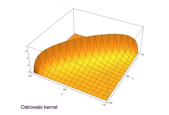
8.1.1. Example 1

Let us consider the Ostrowski’s kernel $K(x,y)$ in (30). As demonstrated by means of the inverse iteration method in [22,23], the relevant operator $\mathcal{T}$ displays the eigenvalues:

$$\begin{array}{c}\hfill \begin{array}{c}{\lambda }_1\simeq 1.205965762856735\hfill \\ {\lambda }_2\simeq 0.734006078303625\hfill \\ {\lambda }_3\simeq 0.528546963103265\hfill \\ {\lambda }_4\simeq 0.413767155184915\hfill \\ {\lambda }_5\simeq 0.342859803772745\hfill \end{array}\end{array}$$

(33)

and, therefore, can be approximated by a matrix of order $r=5$ with a characteristic polynomial:

$$\begin{array}{c}\hfill \begin{array}{c}P(\lambda )=\prod _{k=1}^r\left(\lambda -{\lambda }_k\right).\end{array}\end{array}$$

(34)

Starting from (34), the invariants are readily evaluated as:

$$\begin{array}{c}\hfill \begin{array}{c}{u}_1={\mathcal{I}}_1^1(\mathcal{T})\simeq 3.225145763221285\hfill \\ u_2={\mathcal{I}}_2^1(\mathcal{T})\simeq 3.920164426948163\hfill \\ u_3={\mathcal{I}}_3^1(\mathcal{T})\simeq 2.263632211150296\hfill \\ u_4={\mathcal{I}}_4^1(\mathcal{T})\simeq 0.625036213142174\hfill \\ u_5={\mathcal{I}}_5^1(\mathcal{T})\simeq 0.066372901341124\hfill \end{array}\end{array}$$

(35)

so that the companion matrix $\mathcal{A}$ can be written as:

By making use of the Dunford–Taylor integral Formula (24), the matrix function:

$$\begin{array}{c}\hfill \begin{array}{c}f(\mathcal{A})=W(\mathcal{A})\end{array}\end{array}$$

(36)

with $W(·)$ denoting the product logarithm, can be computed as:

8.1.2. Example 2

Let us consider the kernel $K(x,y)$ relevant to the positive compact operator $\mathcal{T}$ which describes the transverse vibrations of a wedge-shaped beam [24]. By using the inverse iteration method, one can prove that $\mathcal{T}$ features the following eigenvalues:

$$\begin{array}{c}\hfill \begin{array}{c}{\lambda }_1\simeq 1.9717553675\times {10}^{-2}\hfill \\ {\lambda }_2\simeq 1.1930198795\times {10}^{-3}\hfill \\ {\lambda }_3\simeq 2.3684105195\times {10}^{-4}\hfill \\ {\lambda }_4\simeq 7.5156070990\times {10}^{-5}\hfill \\ {\lambda }_5\simeq 3.0836121615\times {10}^{-5}\hfill \\ {\lambda }_6\simeq 1.4889262790\times {10}^{-5}\hfill \\ {\lambda }_7\simeq 8.0483648760\times {10}^{-6}\hfill \\ {\lambda }_8\simeq 4.7300057890\times {10}^{-6}\hfill \\ {\lambda }_9\simeq 2.9688104105\times {10}^{-6}\hfill \\ {\lambda }_{10}\simeq 1.9692639370\times {10}^{-6}\hfill \\ {\lambda }_{11}\simeq 1.3727098565\times {10}^{-6}\hfill \\ {\lambda }_{12}\simeq 1.0037480315\times {10}^{-6}\hfill \\ {\lambda }_{13}\simeq 7.6076195215\times {10}^{-7}\hfill \end{array}\end{array}$$

(37)

and, therefore, can be approximated by a matrix of order $r=13$ with characteristic polynomial:

$$\begin{array}{c}\hfill \begin{array}{c}P(\lambda )=\prod _{k=1}^r(\lambda -{\lambda }_k).\end{array}\end{array}$$

(38)

Starting from (38), the invariants are readily evaluated as:

$$\begin{array}{c}\hfill \begin{array}{c}{u}_1={\mathcal{I}}_1^1(\mathcal{T})\simeq 2.128914972669765\times {10}^{-2}\hfill \\ u_2={\mathcal{I}}_2^1(\mathcal{T})\simeq 3.147982936967773\times {10}^{-5}\hfill \\ u_3={\mathcal{I}}_3^1(\mathcal{T})\simeq 9.746686526750313\times {10}^{-9}\hfill \\ u_4={\mathcal{I}}_4^1(\mathcal{T})\simeq 9.799739677748166\times {10}^{-13}\hfill \\ u_5={\mathcal{I}}_5^1(\mathcal{T})\simeq 4.058777349187134\times {10}^{-17}\hfill \\ u_6={\mathcal{I}}_6^1(\mathcal{T})\simeq 8.015136142635608\times {10}^{-22}\hfill \\ u_7={\mathcal{I}}_7^1(\mathcal{T})\simeq 8.297854829897979\times {10}^{-27}\hfill \\ u_8={\mathcal{I}}_8^1(\mathcal{T})\simeq 4.787022852309753\times {10}^{-32}\hfill \\ u_9={\mathcal{I}}_9^1(\mathcal{T})\simeq 1.593001334376288\times {10}^{-37}\hfill \\ u_{10}={\mathcal{I}}_1^{1}0(\mathcal{T})\simeq 3.084794075371912\times {10}^{-43}\hfill \\ u_{11}={\mathcal{I}}_1^{1}1(\mathcal{T})\simeq 3.391992870896023\times {10}^{-49}\hfill \\ u_{12}={\mathcal{I}}_1^{1}2(\mathcal{T})\simeq 1.945386222042645\times {10}^{-55}\hfill \\ u_{13}={\mathcal{I}}_1^{1}3(\mathcal{T})\simeq 4.485002305839361\times {10}^{-62}\hfill \end{array}\end{array}$$

(39)

so that the companion matrix $\mathcal{A}$ can be written as:

By making use of the Dunford–Taylor integral Formula (24), the matrix function:

$$\begin{array}{c}\hfill \begin{array}{c}{\displaystyle f(\mathcal{A})=\frac{e^{-10\mathcal{A}}}{{\mathcal{A}}^{10}+1}}\end{array}\end{array}$$

(40)

can be computed as:

8.2. Kernels of Inverse of Differential PCO

In [5], many problems relevant to strictly positive definite differential operators have been considered. In particular, for the one connected with the free vibrations of a clamped plate, large numbers of eigenvalues were determined by using the orthogonal invariants method. It is also recalled there that the Fredholm integer function associated with a given kernel $K(x,y)$, where $\mathcal{T}\varphi ={\int }_{A}K(x,y)\varphi (y)dy=\mu \varphi (x)$ is given by:

$$\begin{array}{c}\hfill {\displaystyle G(\mu ,K)=1+\sum _{k=1}^{\infty }{(-1)}^k{\mathcal{I}}_k^1(\mathcal{T}){\mu }^k.}\end{array}$$

(41)

Putting $\lambda ={\mu }^{-1}$, and considering the partial sum, of order r, of the series (30), we recover the polynomial $P(\lambda )$ in Equation (26) as an approximation of the Fredholm integer function (41).

In [5], Fichera, considering the biharmonic operator

$$\begin{array}{c}\hfill {\displaystyle {\Delta }_{4}u(x,y)={\Delta }_2{\Delta }_{2}u=\frac{{\partial }^{4}u}{\partial x^4}+2\frac{{\partial }^{4}u}{\partial x^2\partial y^2}+\frac{{\partial }^{4}u}{\partial y^4}}\end{array}$$

(42)

was able to find lower and upper approximations of the eigenvalues of the biharmonic problem

$$\{\begin{array}{l}{\Delta }_{4}u(x,y)=\lambda u(x,y)\hspace{1em}(\mathrm{in}\mathrm{D})\\ {\displaystyle u=\frac{\partial u}{\partial x}=\frac{\partial u}{\partial y}=0\hspace{1em}(\mathrm{on}\partial \mathrm{D}).}\hfill \end{array}$$

(43)

both for the circular and the square clamped plate.

In what follows, we choose the mean value, as the most probable one, of the very close approximation of the eigenvalues in [5]. Then, considering the reciprocal of these numbers, we apply the results of Section 7 to the inverse operator of the problem (43), which is the relevant Green function, finding, as examples, a few elementary functions of this operator.

8.2.1. Example 3

In the case of a square clamped plate with $\mathrm{D}\equiv \{0\le x\le \pi 0\le y\le \pi \}$, the operator $\mathcal{T}$ which describes the relevant free vibrations features the eigenvalues:

$$\begin{array}{c}\hfill \begin{array}{c}{\lambda }_1\simeq 0.07522320605817612\hfill \\ {\lambda }_2={\lambda }_3\simeq 0.018083584860929095\hfill \\ {\lambda }_4\simeq 0.008318170002599427\hfill \\ {\lambda }_5\simeq 0.005626648256273572\hfill \\ {\lambda }_6\simeq 0.005573530190419659\hfill \\ {\lambda }_7={\lambda }_8\simeq 0.0035787778473651247\hfill \\ {\lambda }_9={\lambda }_{10}\simeq 0.0021993489926981614\hfill \\ {\lambda }_{11}\simeq 0.0020129229654381126\hfill \\ {\lambda }_{12}\simeq 0.0016618597373763058\hfill \end{array}\end{array}$$

(44)

and, therefore, can be approximated by a matrix of order $r=12$ with characteristic polynomial:

$$\begin{array}{c}\hfill \begin{array}{c}P(\lambda )=\prod _{k=1}^r\left(\lambda -{\lambda }_k\right).\end{array}\end{array}$$

(45)

Starting from (45), the invariants are readily evaluated as:

$$\begin{array}{c}\hfill \begin{array}{c}{u}_1={\mathcal{I}}_1^1(\mathcal{T})\simeq 0.146139760612268\hfill \\ u_2={\mathcal{I}}_2^1(\mathcal{T})\simeq 7.435124123661688\times {10}^{-3}\hfill \\ u_3={\mathcal{I}}_3^1(\mathcal{T})\simeq 1.923841312742190\times {10}^{-4}\hfill \\ u_4={\mathcal{I}}_4^1(\mathcal{T})\simeq 2.933369354737111\times {10}^{-6}\hfill \\ u_5={\mathcal{I}}_5^1(\mathcal{T})\simeq 2.845078672719340\times {10}^{-8}\hfill \\ u_6={\mathcal{I}}_6^1(\mathcal{T})\simeq 1.830841553974511\times {10}^{-10}\hfill \\ u_7={\mathcal{I}}_7^1(\mathcal{T})\simeq 7.975992951293202\times {10}^{-13}\hfill \\ u_8={\mathcal{I}}_8^1(\mathcal{T})\simeq 2.357390178302073\times {10}^{-15}\hfill \\ u_9={\mathcal{I}}_9^1(\mathcal{T})\simeq 4.646069994825235\times {10}^{-18}\hfill \\ u_{10}={\mathcal{I}}_1^{1}0(\mathcal{T})\simeq 5.833548132502803\times {10}^{-21}\hfill \\ u_{11}={\mathcal{I}}_1^{1}1(\mathcal{T})\simeq 4.213005422976779\times {10}^{-24}\hfill \\ u_{12}={\mathcal{I}}_1^{1}2(\mathcal{T})\simeq 1.329866701687217\times {10}^{-27}\hfill \end{array}\end{array}$$

(46)

so that the companion matrix $\mathcal{A}$ can be written as:

By making use of the Dunford–Taylor integral Formula (24), the matrix function:

$$\begin{array}{c}\hfill \begin{array}{c}{\displaystyle f(\mathcal{A})=log(\mathcal{A})}\end{array}\end{array}$$

(47)

can be computed as:

8.2.2. Example 4

In the case of a circular clamped plate with $\mathrm{D}\equiv x^2+y^2\le 1$, the operator $\mathcal{T}$ which describes the relevant free vibrations features the eigenvalues:

$$\begin{array}{c}\hfill \begin{array}{c}{\lambda }_1\simeq 0.009581894052997456\hfill \\ {\lambda }_2={\lambda }_3\simeq 0.0022123673547497866\hfill \\ {\lambda }_4\simeq 0.0008220946148692253\hfill \\ {\lambda }_5\simeq 0.005626648256273572\hfill \\ {\lambda }_6\simeq 0.0006322131569880101\hfill \\ {\lambda }_7={\lambda }_8\simeq 0.00038401499194528553\hfill \\ {\lambda }_9={\lambda }_{10}\simeq 0.00027026150503226925\hfill \end{array}\end{array}$$

(48)

and, therefore, can be approximated by a matrix of order $r=10$ with characteristic polynomial:

$$\begin{array}{c}\hfill \begin{array}{c}P(\lambda )=\prod _{k=1}^r\left(\lambda -{\lambda }_k\right).\end{array}\end{array}$$

(49)

Starting from (49), the invariants are readily evaluated as:

$$\begin{array}{c}\hfill \begin{array}{c}{u}_1={\mathcal{I}}_1^1(\mathcal{T})\simeq 2.239613778458294\times {10}^{-2}\hfill \\ u_2={\mathcal{I}}_2^1(\mathcal{T})\simeq 1.834047170883283\times {10}^{-4}\hfill \\ u_3={\mathcal{I}}_3^1(\mathcal{T})\simeq 7.231844608387320\times {10}^{-7}\hfill \\ u_4={\mathcal{I}}_4^1(\mathcal{T})\simeq 1.549026411656578\times {10}^{-9}\hfill \\ u_5={\mathcal{I}}_5^1(\mathcal{T})\simeq 1.916470543643900\times {10}^{-12}\hfill \\ u_6={\mathcal{I}}_6^1(\mathcal{T})\simeq 1.421413780191233\times {10}^{-15}\hfill \\ u_7={\mathcal{I}}_7^1(\mathcal{T})\simeq 6.388300810511680\times {10}^{-19}\hfill \\ u_8={\mathcal{I}}_8^1(\mathcal{T})\simeq 1.698427046738193\times {10}^{-22}\hfill \\ u_9={\mathcal{I}}_9^1(\mathcal{T})\simeq 2.451210499521412\times {10}^{-26}\hfill \\ u_{10}={\mathcal{I}}_1^{1}0(\mathcal{T})\simeq 1.477289762215714\times {10}^{-30}\hfill \end{array}\end{array}$$

(50)

so that the companion matrix $\mathcal{A}$ can be written as:

By making use of the Dunford–Taylor integral Formula (24), the matrix function:

$$\begin{array}{c}\hfill \begin{array}{c}{\displaystyle f(\mathcal{A})={tan}^{-1}(\mathcal{A})}\end{array}\end{array}$$

(51)

can be computed as:

9. Conclusions

The use of Bell polynomials allows for extending to a countable set of numbers the Newton–Girard formulas originally stated in the framework of polynomials.

Then, the Robert’s formulas for the orthogonal invariants of a positive compact operator are recognized as the recursion or the Faà di Bruno [25] formula for the Bell polynomials. Therefore, the reduction of the order (or the grade) of the orthogonal invariants is easily established.

By using the results on matrix functions, based on the Dunford–Taylor integral, an approximation to holomorphic function of positive compact operators is obtained considering a truncation of Fredholm’s integral function whose coefficients are precisely the orthogonal invariants of the PCO. This is possible since the eigenvalues of such operators often tend to zero in a very fast way so that a finite set of eigenvalues gives a sufficient idea of the behavior of the considered function. Numerical examples obtained by using the computer algebra program Mathematica${}^{\copyright }$ are included. The results matches with the theoretical approach.

References

- Bell, E.T. Exponential polynomials. Ann. Mathematics 1934, 35, 258–277. [Google Scholar] [CrossRef]
- Riordan, J. An Introduction to Combinatorial Analysis; J. Wiley & Sons: Chichester, UK, 1958. [Google Scholar]
- Bruschi, M.; Ricci, P.E. I polinomi di Lucas e di Tchebycheff in più variabili. Rend. Mat. 1980, 13, 507–530. [Google Scholar]
- Cassisa, C.; Ricci, P.E. Orthogonal invariants and the Bell polynomials. Rend. Mat. Appl. 2000, 20, 293–303. [Google Scholar]
- Fichera, G. Abstract and Numerical Aspects of Eigenvalue Theory; Lecture Notes; Department of Mathematics, The University of Alberta: Edmonton, AB, Canada, 1973. [Google Scholar]
- Fichera, G. Metodi e risultati concernenti l’analisi numerica e quantitativa. Atti Accad. Nazion. Lincei Mem. 1974, 7, 1–202. [Google Scholar]
- Caratelli, D.; Ricci, P.E. A Numerical Method for Computing the Roots of Non-Singular Complex-Valued Matrices. Symmetry 2020, 12, 966. [Google Scholar] [CrossRef]
- Dodds, P.G. Positive compact operators. Quaest. Math. 1995, 18, 21–45. [Google Scholar] [CrossRef]
- Osborn, J.E. Spectral Approximation for Compact Operators. Math. Comput. 1975, 29, 712–715. [Google Scholar] [CrossRef]
- Zerner, M. Quelques propriétés spectrales des opérateurs positifs. J. Funct. Anal. 1987, 72, 381–417. [Google Scholar] [CrossRef][Green Version]
- Roman, S.M. The Faà di Bruno Formula. Am. Math. Mon. 1980, 87, 805–809. [Google Scholar] [CrossRef]
- Roman, S.M.; Rota, G.C. The umbral calculus. Adv. Math. 1978, 27, 95–188. [Google Scholar] [CrossRef]
- Comtet, L. Advanced Combinatorics: The Art of Finite and Infinite Expansions; D. Reidel Publishing Co.: Dordrecht, The Netherlands, 1974; Available online: https://doi.org/10.1007/978-94-010-2196-8 (accessed on 12 February 2020).
- Kurosh, A. Cours d’Algèbre Supérieure; Éditions Mir: Moscou, Russia, 1971. [Google Scholar]
- Mikhlin, S.G. Integral Equations and Their Applications, 2nd ed.; Pergamon Press: Oxford, UK, 1964. [Google Scholar]
- Tricomi, F.G. Su di una classe di nuclei definiti positivi. Boll. Dell’Unione Mat. Ital. 1967, 22, 1–3. [Google Scholar]
- Robert, D. Invariants orthogonaux pour certaines classes d’operateurs. Ann. Mathém. Pures Appl. 1973, 52, 81–114. [Google Scholar]
- Kato, T. Perturbation Theory for Linear Operators; Springer: Berlin/Heidelberg, Germany, 1966. [Google Scholar]
- Bruschi, M.; Ricci, P.E. An explicit formula for f(A) and the generating function of the generalized Lucas polynomials. SIAM J. Math. Anal. 1982, 13, 162–165. [Google Scholar] [CrossRef]
- Caratelli, D.; Ricci, P.E. A note on integer powers of a Companion matrix and Applications. Tbilisi Math. J. 2020. to appear. [Google Scholar]
- Krall, G. Meccanica Tecnica Delle Vibrazioni; Veschi: Roma, Italy, 1970; Volume I. [Google Scholar]
- Fichera, G.; Sneider, M.A. Un problema di autovalori proposto da Alexander M. Ostrowski. Rend. Mat. 1975, 8, 201–224. [Google Scholar]
- Natalini, P.; Noschese, S.; Ricci, P.E. An iterative method for computing the eigenvalues of second kind Fredoholm operators and applications. Electron. Trans. Numer. Anal. 1999, 9, 128–136. [Google Scholar]
- Belingeri, C.; Germano, B. Numerical approximation of eigenvalues for transverse vibrations of a wedge-shaped beam. Appl. Math. Inf. Tbil. 1999, 4, 1–10. [Google Scholar]
- Faà di Bruno, F. Théorie des Formes Binaires; Brero: Turin, Italy, 1876. [Google Scholar]
© 2020 by the authors. Licensee MDPI, Basel, Switzerland. This article is an open access article distributed under the terms and conditions of the Creative Commons Attribution (CC BY) license (http://creativecommons.org/licenses/by/4.0/).