Study on Improvement of Lightning Damage Detection Model for Wind Turbine Blade

Abstract

There have been many reports of damage to wind turbine blades caused by lightning strikes in Japan. In some of these cases, the blades struck by lightning continue to rotate, causing more serious secondary damage. To prevent such accidents, it is a requirement that a lightning detection system is installed on the wind turbine in areas where winter lightning occurs in Japan. This immediately stops the wind turbine if the system detects a lightning strike. Normally, these wind turbines are restarted after confirming soundness of the blade through visual inspection. However, it is often difficult to confirm the soundness of the blade visually for reasons such as bad weather. This process prolongs the time taken to restart, and it is one of the causes that reduces the availability of the wind turbines. In this research, we constructed a damage detection model for wind turbine blades using machine learning based on SCADA system data and, thereby, considered whether the technology automatically confirms the soundness of wind turbine blades.

1. Introduction

The efforts to realize a low-carbon society are being promoted against the background of global environmental issues, which are of increasing interest around the world. As one of the attempts to reduce carbon production, countries are expanding the use of renewable energy such as wind power generation, solar power generation, and geothermal power generation. Among them, wind power generation including offshore is attracting attention as a cost-effective power generation method, and it is under extensive development around the world.

However, many wind turbines in Japan have received serious damage caused by lightning strikes, and it is regarded as a problem. The wind turbines in Japan are under conditions that are vulnerable to lightning strikes, because a quarter of the wind turbines are built on the Sea of Japan coast where large lightning strikes are likely to occur and wind turbines are getting bigger. The wind turbine blades receiving lightning strikes are often catastrophically damaged with cracks. Accidents have been reported in which the rotating blade received such damage and the damage gradually expanded due to centrifugal force, leading to more serious secondary damage [1,2,3]. Research on lightning protection measures to prevent such lightning damage is being actively conducted [4,5,6,7,8,9].

The Japanese ministry of economy, trade and industry partially revised its interpretation of technical standards for wind power generation equipment to prevent such accidents. It was decided in the revision to install an emergency stop device so that the wind turbine can be stopped immediately if the lightning strike hits the wind turbine in the winter lightning area of the Sea of Japan coast [10]. By this revision, the wind turbines must be emergency stopped if the lightning detection system (LDS) installed on the wind turbine detects a lightning strike, and it can no longer be restarted until it is confirmed to be sound. Normally, the soundness of the wind turbine is confirmed by visual inspection by workers, but it often takes a long time to restart because quick visual inspection becomes difficult due to bad weather. Such a prolonged downtime is a factor that reduces availability of wind turbine. One wind farm could not be restarted immediately after a lightning strike on a wind turbine due to weather or other reasons, and the availability dropped by 2.23% over the year [11]. If the soundness of the wind turbine is impaired by a lightning strike, it is necessary to grasp the situation and restart after repair. However, if the soundness of the wind turbine is maintained despite the lightning strike hitting the wind turbine, it is necessary to restart as quickly as possible and improve the availability.

We propose that a lightning damage detection model for wind turbine can be constructed using supervisory control and data acquisition system data (SCADA data) as a feature of the machine learning model. It is expected that the operation will be restated quickly after a lightning strike is detected because it does not require visual inspection by workers if the soundness of the blade can be confirmed based on SCADA data, and that the availability will be improved accordingly. Furthermore, the anomaly detection models using SCADA data have the advantage of not requiring additional equipment while the existing blade damage detection method [12,13] requires additional equipment such as vibration sensors. The SCADA system is installed on all wind turbines and the system can collect data of the wind turbine remotely. Therefore, the soundness of the blade can be confirmed remotely in real time with the existing equipment if the SCADA system is used for anomaly detection.

A study on an anomaly detection method for wind turbines based on SCADA data is being constructed [14,15,16]. Among them, it was clarified that it can detected anomalies of the wind turbine by a machine learning model that has features such as power curve and rotational speed of wind turbine. However, this method aims to predict failure due to deterioration over time from months to weeks in advance, and it is not applicable to sudden damage such as lightning damage. Therefore, our research group proposed the method that can immediately detect blade anomalies caused by a sudden event such as a lightning strike [17]. Accordingly, it is necessary to continue to consider the optimal anomaly detection model and effective features based on this result.

In this paper, we describe a lightning damage detection model for wind turbine blades using a Gaussian mixture model (GMM). Additionally, we report the method that can detect blade anomalies due to lightning strikes automatically and results of examination about the method to improve detection accuracy. This paper consists of the following four sections. Section 2 describes the feature extraction method, learning method, and assessment method of the lightning damage detection model for wind turbine blade. In Section 3, we will examine the anomaly detection accuracy and reliability of this model using SCADA data of a wind turbine whose blades have been damaged by a lightning strike. In Section 4, we compare the anomaly detection accuracy of multiple models and examine the accuracy improvement. Finally, we conclude the paper in Section 5. In addition, Table 1 lists symbols, acronyms and abbreviations used in this paper.

Table 1. List of symbols, acronyms and abbreviations.

LDS	Lightning Detection System
SCADA	Supervisory control and data acquisition
GMM	Gaussian mixture model
BIC	Bayesian information criterion
ROC	Receiver operating characteristic
AUC	Area under the curve
SMA	Simple moving average
WMA	Weighted moving average
EMA	Exponential moving average
SWMA	Sine weighted moving average
MMA	Size of window
α	Weight factor of exponential moving average
n	Number of the data
x	Data
$\mathcal{N} \left({\mathit{x}|\mathit{\mu }}_{\mathit{k}},{\Sigma }_{\mathit{k}}\right)$	Gaussian distribution k
$\mathit{p}\left(\mathit{x}\right|\Theta )$	Gaussian mixture model
πk	Weighting coefficient of the Gaussian distribution k
μk	Mean vector of the Gaussian distribution k
Σk	General covariance matrix of the Gaussian distribution k
Θ	Set of three parameters πk, μk, Σk
K	Total number of Gaussian distributions
$L\left(\Theta \right)$	Log-likelihood probability on Θ
γ	Posterior probability
score	Anomaly score
TP	True positive
FP	False positive
TN	True negative
FN	False negative

2. Construction of Lightning Damage Detection Model for Wind Turbine Blades

2.1. Process of Training and Assessment for the Model

In this study, the lightning damage detection model for wind turbine blades was trained and assessed using SCADA data of the wind turbines. This wind turbine was reported blade damage accident caused by a lightning strike. Figure 1 shows the process of training and assessment for the model.

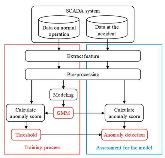
Figure 1. Process of training and assessment.

In the training process of the model, GMM is trained using the data on normal operation of the wind turbine. It is possible to calculate the degree of deviation from normal value as anomaly score by modeling the data on normal operation. Additionally, the threshold of the anomaly score is determined using anomaly score on normal operation calculated by the trained GMM.

In the assessment process, the anomaly detection accuracy of the trained GMM is assessed using the data at the accident. First, the anomaly score at the accident is calculated using the trained GMM, and hence, normal or abnormal are discriminated by the threshold. The data at the accident are labeled in advance as normal immediately before the lightning strike and abnormal immediately after the lightning strike. Accordingly, this is used as the true label and compared with the anomaly detection result to assess the accuracy.

2.2. Extraction of Feature

2.2.1. SCADA System

SCADA systems are used to remotely monitor the current status of wind turbines such as wind speed, wind direction, rotational speed, power, and component temperatures. The system installed on most modern wind turbines can collect data every second, but many business operators store only data averaged to 1 min or 10 min because the amount of the data would be too large otherwise.

2.2.2. SCADA Data of Wind Turbine at the Accident Due to Lightning Strike

It was clarified in previous research [17] that, if a wind turbine blade is damaged by a lightning strike, the outliers will occur frequently and continuously in wind speed rotational speed characteristic, wind speed power characteristic, and wind speed pitch degree characteristis of SCADA data. Based on this result, anomaly detection is performed using the wind speed rotational speed characteristic, which show the most outliers.

Figure 2 shows wind speed-rotational speed characteristic of 1 min averaged SCADA data collected from the wind turbine. This wind turbine blade have been damaged by a lightning strike. Table 2 shows the data acquisition period of Figure 2. In the graphs, the blue dots represent the data immediately before the lightning strike, the red dots represent the data immediately after the lightning strike, and the green dots represent the data on normal operation. Additionally, data that deviate from the overall tendency (outliers) are surrounded by a black frame.

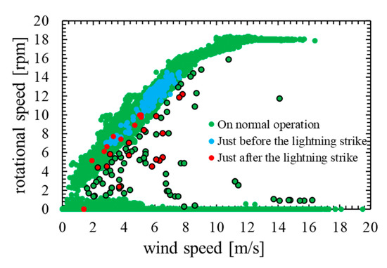
Figure 2. Wind speed rotational speed characteristic.

Table 2. Data acquisition period of SCADA data.

Type of SCADA Data	Data Period
	at the Accident	on Normal Operation
1 min average data	170 min	The data after repair for about 33 days

As shown in Figure 2, most data immediately after the lightning strike are outliers. However, outliers also occur in data on normal operation, and hence, the data immediately after the lightning strike and the data on normal operation are not linearly separable. Therefore, anomaly detection using threshold is difficult, and it is considered that the method based on machine learning model is effective.

It is necessary to clarify the difference between the outliers that occur immediately after a lightning strike and the outliers that occur during normal operation by confirming the time characteristics of the rotational speed. Figure 3 shows time characteristics of rotational speed on normal operation. Figure 4 shows time characteristics of rotational speed before and after the lightning strike.

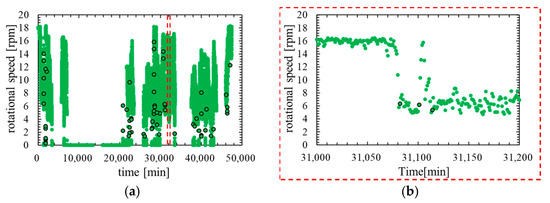
Figure 3. Time characteristic of rotational speed in normal operation: (a) rotational speed on normal operation; (b) rotational speed on normal operation (partial expansion).

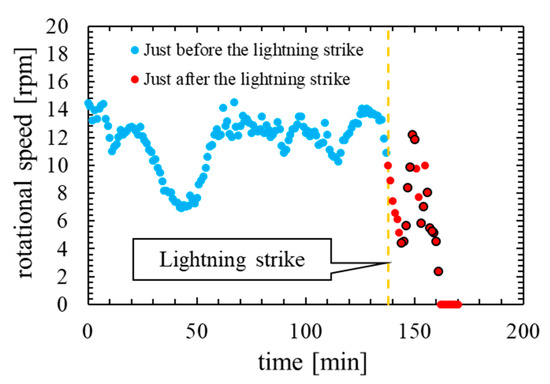
Figure 4. Time characteristic of rotational speed at the accident.

In comparing Figure 3 and Figure 4, the outliers that occur on normal operation are not consecutive three times or more. By contrast, the outliers that occur immediately after the lightning strike are continuous for several minutes. Therefore, it is considered that the abnormal data immediately after the lightning strike can be detected by reflecting the frequency of outliers in the feature of the anomaly detection model.

2.2.3. Extraction Method for Features Using Moving Average

According to study result in Section 2.2.2, it is necessary to consider the time characteristics, rather than simply using wind speed and rotational speed as features. Therefore, we select multiple moving averages of wind speed and rotational speed as features. It is considered that temporal characteristics can be included in the features by using the moving average because the moving average is calculated using the data for a few minutes.

In this study, we used a simple moving average, a weighted moving average, an exponential moving average, and a sine weighted moving average. Each moving average is shown in Equations (1) to (4). In these Equations, x_i means the i-th data. Here, M_MA = 5, α = 0.1.

$${\mathit{SMA}}_n=\frac{1}{M_{\mathit{MA}}}{\displaystyle \sum }_{{i=n-M}_{\mathit{MA}}+1}^n{x}_i$$

(1)

$${\mathit{WMA}}_n=\frac{2}{M_{\mathit{MA}}{(M}_{\mathit{MA}}+1)}{\displaystyle \sum }_{{i=n-M}_{\mathit{MA}}+1}^n{i x}_i$$

(2)

$${\mathit{EMA}}_n{=\mathit{EMA}}_{n-1}+\alpha (x_i-{\mathit{EMA}}_{n-1})$$

(3)

$${\mathit{SWMA}}_n=\frac{{{\displaystyle \sum }}_{{i=n-M}_{\mathit{MA}}+1}^n{x}_i\sin \left(\frac{i}{M_{\mathit{MA}}+1}\mathsf{\pi }\right)}{{{\displaystyle \sum }}_{{i=n-M}_{\mathit{MA}}+1}^n\sin \left(\frac{i}{M_{\mathit{MA}}+1}\mathsf{\pi }\right)}$$

(4)

The wind speed and rotational speed were converted into features using the Equations (1) to (4). Consequently, features are 2 × 5 dimensions. As shown in Equations (1), (2) and (4), feature includes information of the data for M_MA minutes. Additionally, as shown in Equation (3), feature includes information of all past data.

2.2.4. Pre-Processing for Features

In this study, the feature is 0–1 normalized so that the maximum value is 1 and the minimum value is 0, as shown in Equation (5).

$${x_n}^{\prime }=\frac{x_n-\min \mathit{x}}{\max \mathit{x}-\min \mathit{x}}$$

(5)

The data when rotational speed is 0 rpm is removed from training data and assessment data, because wind speed will be the only effective feature in this anomaly detection model when the blade is stopped. In this case, the anomaly detection for wind speed is performed, but the anomaly detection for wind turbines is not performed properly. For this reason, it is not appropriate that to use the data when the blade is stopped for this model.

2.3. Anomaly Detection Model Using GMM

2.3.1. Theoretical Explanation of GMM

In this study, the lightning damage detection model for wind turbine blades is constructed using GMM. GMM can estimate the probabilistic model based on data density of normal data and discriminates areas with low data density as abnormal [18]. As is clear from the study results in Section 2.2.2, the data density is low in the area where outliers occur. Hence, it is considered that anomaly detection by GMM is effective. Furthermore, GMM can be trained using only normal data, and hence, does not require abnormal data for training. Therefore, GMM is appropriate method for detecting lightning damage because the data when the blade is damaged by lightning strike are scarce.

The basic equations of GMM are shown in Equations (6) to (9).

$$\mathit{p}\left(\mathit{x}\right|\mathbf{\Theta })={\displaystyle \sum }_{k=1}^K{\mathsf{\pi }}_k\mathcal{N}\left(\mathit{x}\right|{\mathit{\mu }}_{\mathit{k}}{,\mathsf{\Sigma }}_{\mathit{k}})$$

(6)

$$\mathcal{N} \left(x|{\mathit{\mu }}_{\mathit{k}},{\mathsf{\Sigma }}_{\mathit{k}}\right)=\frac{\exp \left(-\frac{1}{2}{(\mathit{x}-{\mathit{\mu }}_{\mathit{k}})}^{\mathrm{T}}{\mathsf{\Sigma }}_{\mathit{k}}^{-1}(\mathit{x}-{\mathit{\mu }}_{\mathit{k}})\right)}{{(2\mathsf{\pi }\left|{\mathsf{\Sigma }}_{\mathit{k}}\right|)}^{\frac{d}{2}}}$$

(7)

$$0\le {\mathsf{\pi }}_k\le 1$$

(8)

$${\displaystyle \sum }_{k=1}^K{\mathsf{\pi }}_k=1$$

(9)

As shown in Equations (6) and (7), GMM is represented by sum of weighted Gaussian distributions. GMM can estimate the probabilistic model that d-dimensional data x follows, where π_k is the weighting coefficient of the Gaussian distribution k, besides, μ_k and Σ_k are the mean vector and the general covariance matrix of the Gaussian distribution k. Θ is represented as the set of these three parameters π_k, μ_k, Σ_k for each Gaussian distribution. K means the total number of Gaussian distributions, and it is a hyperparameter of the GMM. $\mathit{p}\left(\mathit{x}\right|\mathbf{\Theta })$ estimated by GMM can be treated as probability density function, because sum of weighting coefficient π is limited to 1 as shown in equations (8) and (9). Therefore, it becomes 1 when the $\mathit{p}\left(\mathit{x}\right|\mathbf{\Theta })$ is integrated over the entire interval of x.

GMM parameter Θ can be optimized by maximizing log-likelihood probability defined by Equation (10), where N is total number of the data.

$$L\left(\mathbf{\Theta }\right)=\ln {\displaystyle \prod }_{i=0}^N\mathit{p}({\mathit{x}}_{\mathit{i}}\left|\mathbf{\Theta }\right)$$

(10)

The expectation-maximization algorithm (EM algorithm) [19] is used to maximize the log-likelihood probability of Equation (10). For the calculation of the EM algorithm, posterior probability γ calculated by Equation (11) and renewal formula shown in Equations (12) to (14) are used. First, we randomly decide the initial values of π_k, μ_k, and Σ_k, and thus, calculate the posterior probability γ by Equation (11). Second, we update π_k, μ_k, and Σ_k using Equations (12) to (14). Note that the μ_k in Equation (14) is updated one. This posterior probability calculation and parameter update are repeated until the parameters converge, so that the log-likelihood probability can be maximized.

$${\mathsf{\gamma }}_{nk}=\frac{{\mathsf{\pi }}_k\mathcal{N}\left({\mathit{x}}_{\mathit{n}}\right|{\mathit{\mu }}_{\mathit{k}},{\Sigma }_k)}{{{\displaystyle \sum }}_{k=1}^K{\mathsf{\pi }}_k\mathcal{N}\left({\mathit{x}}_{\mathit{n}}{|\mathit{\mu }}_{\mathit{k}}{,\Sigma }_{\mathit{k}}\right)}$$

(11)

$${\mathsf{\pi }}_k=\frac{{{\displaystyle \sum }}_{n=1}^N{\mathsf{\gamma }}_{nk} }{N}$$

(12)

$${\mathit{\mu }}_{\mathit{k}}=\frac{{{\displaystyle \sum }}_{n=1}^N{\mathsf{\gamma }}_{nk}{ \mathit{x}}_{\mathit{n}}}{{{\displaystyle \sum }}_{n=1}^N{\mathsf{\gamma }}_{nk}}$$

(13)

$${\mathsf{\Sigma }}_{\mathit{k}}=\frac{{{\displaystyle \sum }}_{n=1}^N{\mathsf{\gamma }}_{nk} \left({\mathit{x}}_{\mathit{n}}-{\mathit{\mu }}_{\mathit{k}}\right){\left({\mathit{x}}_{\mathit{n}}-{\mathit{\mu }}_{\mathit{k}}\right)}^{\mathrm{T}}}{{{\displaystyle \sum }}_{n=1}^N{\mathsf{\gamma }}_{nk} }$$

(14)

2.3.2. Anomaly Detection by GMM

It is necessary to define anomaly score based on probability density for performing anomaly detection using GMM. The predicted distribution p(x|Θ) of the normal data will be obtained if only normal data are modeled by GMM. Using this predicted distribution, the probability density p(x⁽ⁿ⁾|Θ) of arbitrary data x⁽ⁿ⁾ can be calculated. p(x⁽ⁿ⁾|Θ) will low if x⁽ⁿ⁾ is abnormal data since abnormal data is unlikely to occur. The anomaly score is defined by Equation (15) below utilizing this property. Equation (15) is the negative logarithm of the probability density, and thus the anomaly score will increase if the probability of occurrence is low such as abnormal data.

$$score=-\ln p({\mathit{x}}^{\left(\mathit{n}\right)}|\mathbf{\Theta })$$

(15)

It is possible to discriminate between normal data and abnormal data if a threshold is set for the anomaly score calculated by Equation (15).

2.3.3. Selection of Hyperparameter K of GMM

The number of mixture components K must be determined in advance to train GMM. In this study, we compared the following two selection methods and examined the imsprovement of anomaly detection accuracy.

Normally, the Bayesian information criterion (BIC) [19] shown in Equation (16) is used to select K. where k_p is number of features. As shown in Equation (16), BIC becomes smaller as the probability distribution fits the data. In this study, we used a method that automatically selects the K with the lowest BIC between 2 and 256.

$$\mathit{BIC}=-{2\ln p\left(\mathit{x}\right|\Theta )+k}_p\ln \left(N\right)$$

(16)

On the other hand, when using GMM as an anomaly detection method, it is also effective as a method of selecting the most accurate K by comparing anomaly detection accuracy on multiple K. BIC is an evaluation standard proposed to select the appropriate model for the cluster analysis method. Therefore it is effective for data divided into multiple classes [18]. However, GMM is used as a method for estimating the predicted distribution of data in this study, thus the BIC of the best model for anomaly detection is not always low. Accordingly, there is a high possibility that the anomaly detection accuracy can be improved by selecting a model based on the anomaly detection accuracy itself, rather than based on BIC. In this study, we set K to 64, 128 and 256 to compare these anomaly detection accuracies.

2.3.4. Assessment for Anomaly Detection Accuracy

In this study, anomaly detection accuracy of the model is assessed using confusion matrix and the receiver operating characteristic curve (ROC curve). Below is a brief description of the confusion matrix and ROC curve.

The confusion matrix shown in Table 3 summarizes true positive, false positive, true negative, and false negative [20]. Normally, anomaly detection accuracy cannot be sufficiently assessed by simply calculating the correct answer rate because the ratio of abnormal assessment data for the anomaly detection model is extremely small. It is possible to consider the bias of the data by using confusion matrix because normal data and abnormal data can be represented separately.

Table 3. Confusion matrix.

		Predicted
		Abnormal	Normal
True	Abnormal	True positive (TP)	False negative (FN)
	Normal	False positive (FP)	True negative (TN)

The ROC curve shows the locus of the false positive rate-true positive rate characteristic when the threshold is changed [20]. True positive rate and false positive rate can be calculated by the following Equations (17) and (18). The area surrounded by a straight line with false positive rate = 1, a straight line with true positive rate = 0, and the ROC curve is called Area Under the Curve (AUC). As is clear from the definition of the ROC curve, the AUC expands as the anomaly detection accuracy increases. Thereby, the AUC is assessment standard for performance of the model. Note that the range of AUC is 0 to 1.

$$\mathrm{True} \mathrm{positive} \mathrm{rate}=\frac{TP}{TP+FN}$$

(17)

$$\mathrm{False} \mathrm{positive} \mathrm{rate}=\frac{FP}{FP+TN}$$

(18)

3. Result of Anomaly Detection and Performance Assessment

3.1. The Model in Which the Number of Mixture Components K Was Determined Based on BIC

This model automatically selected the K with the lowest BIC between 2 and 256 and performed anomaly detection. Besides, the 99th percentile value of the anomaly score calculated from the data during normal operation was used as the threshold. It should be noted the selected K was 29.

Figure 5 shows the assessment result of this model. In Figure 5a,b, the blue dots represent the data immediately before the lightning strike, and the red dots represent the data immediately after the lightning strike. In the Figure 5c,d, the blue dots represent the data that the model predicted to be normal, and the red dots represent the data that the model predicted to be abnormal. Additionally, X is plotted against the data that were poorly predicted. Figure 5e shows the time characteristics of the anomaly score and its threshold.

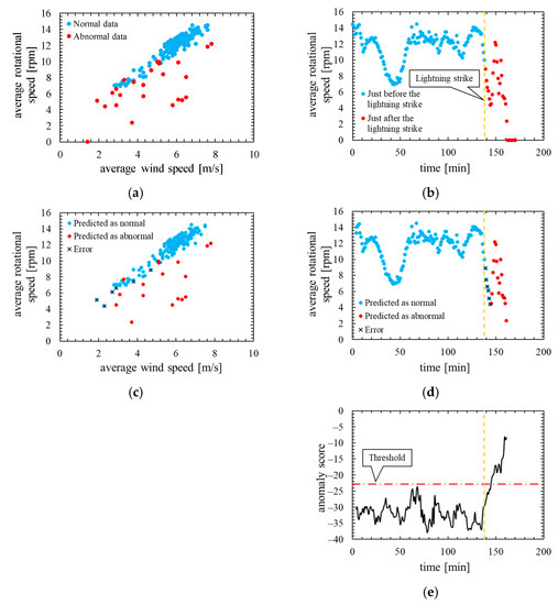
Figure 5. True label and assessment result of the model in which the number of mixture components K was determined based on BIC (K = 29, threshold is 99th percentile’s value): (a) wind speed-rotational speed characteristic with true label; (b) time characteristics of rotational speed with true label; (c) wind speed rotational speed characteristic with predicted label; (d) time characteristics of rotational speed with predicted label; (e) time characteristics of anomaly score.

This result is assessed by the confusion matrix and the ROC curve. Table 4 shows the confusion matrix, and Figure 6 shows the ROC curve.

Table 4. Confusion matrix of the model in which the number of mixture components K was determined based on BIC (K = 29, the threshold is the 99th percentile’s value).

		Predicted
		Abnormal	Normal
True	Abnormal	17	6
	Normal	0	135

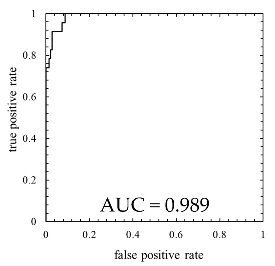
Figure 6. ROC curve of the model in which the number of mixture components K was determined based on BIC (K = 29, the threshold is the 99th percentile’s value).

Next, Figure 7 shows the training data of this model. In Figure 7a,b, the red dots represent the data that exceed the threshold. Figure 7c shows the time characteristics of the anomaly score and its threshold.

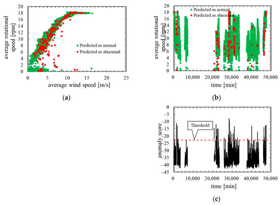
Figure 7. Training data of the model in which the number of mixture components K was determined based on BIC (K = 29, the threshold is the 99th percentile’s value): (a) wind speed rotational speed characteristic; (b) time characteristics of rotational speed; (c) time characteristics of anomaly score.

As is clear from Figure 5, anomaly score increases immediately after the lightning strike and exceeds the threshold. Consequently, the data immediately after the lightning strike is properly detected as abnormal. As shown in ROC curve of Figure 6, AUC is more than 0.9, indicating that anomaly detection was performed appropriately. Additionally, Table 4 indicates that six false negatives occurred. These six data are for 6 minutes after a lightning strike, and, hence, it is considered that there is a time delay before the abnormal data is detected. As shown in Figure 7, an increase in the anomaly score is seen even data on normal operation, thereby false positives are likely to occur.

3.2. The Model in Which the Number of Mixture Components K Was 64

This model performed anomaly detection with K set to 64. The 100th percentile value of the anomaly score calculated from the data during normal operation was used as the threshold.

Figure 8 shows the assessment result of this model. Note that, the layout and the types of plots of the Figure 8 are the same as in Figure 5.

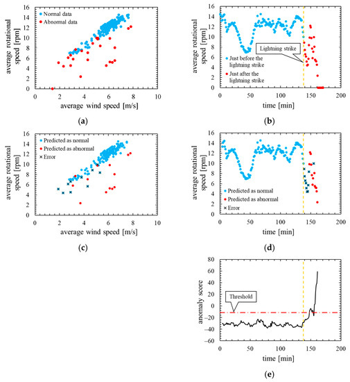
Figure 8. True label and assessment result of the model in which the number of mixture components K was 64 (threshold is the 100th percentile’s value): (a) wind speed rotational speed characteristic with true label; (b) time characteristics of rotational speed with true label; (c) wind speed rotational speed characteristic with predicted label; (d) time characteristics of rotational speed with predicted label; (e) time characteristics of anomaly score.

This result is assessed by the confusion matrix and the ROC curve. Table 5 shows the confusion matrix, and Figure 9 shows the ROC curve.

Table 5. Confusion matrix of the model in which the number of mixture components K was 64 (the threshold is the 100th percentile’s value).

		Predicted
		Abnormal	Normal
True	Abnormal	13	10
	Normal	0	135

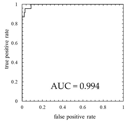
Figure 9. ROC curve of the model in which the number of mixture components K was 64 (the threshold is the 100th percentile’s value).

Next, Figure 10 shows the training data of this model. Note that, the layout and the types of plots of the Figure 10 are the same as in Figure 7.

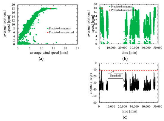
Figure 10. Training data of the model in which the number of mixture components K was 64 (the threshold is 100th percentile’s value): (a) wind speed rotational speed characteristic; (b) time characteristics of rotational speed; (c) time characteristics of anomaly score.

As is clear from Figure 8, anomaly score increases immediately after the lightning strike and exceeds the threshold. Consequently, the data immediately after the lightning strike are properly detected as abnormal. However, the anomaly score after the lightning strike decreased temporarily and fell below the threshold so that the false negative occurred. As shown in ROC curve of Figure 9, AUC is more than 0.99, indicating that anomaly detection was performed appropriately. Additionally, Table 5 indicates that 10 false negatives occurred. These 10 data are due to the time delay of anomaly detection and the decrease in the anomaly score after a lightning strike. As shown in training data of Figure 10, the anomaly score during normal operation is stable and there is no sharp rise like immediately after a lightning strike, and hence, it is considered that the false positives are unlikely to occur.

3.3. The Model in Which the Number of Mixture Components K Was 128

This model performed anomaly detection with K set to 128. The 100th percentile’s value for the anomaly score calculated from the data during normal operation was used as the threshold.

Figure 11 shows the assessment result of this model. Note that, the layout and the types of plots of the Figure 11 are the same as in the assessment result of the other models.

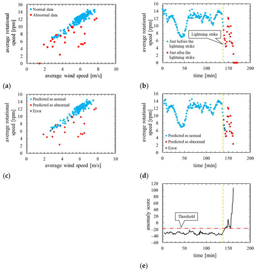
Figure 11. True label and assessment result of the model in which the number of mixture components K was 128 (the threshold is the 100th percentile’s value): (a) wind speed rotational speed characteristic with true label; (b) time characteristics of rotational speed with true label; (c) wind speed-rotational speed characteristic with predicted label; (d) time characteristics of rotational speed with predicted label; (e) time characteristics of anomaly score.

This result is assessed by the confusion matrix and the ROC curve. Table 6 shows the confusion matrix, and Figure 12 shows the ROC curve.

Table 6. Confusion matrix of the model in which the number of mixture components K was 128 (threshold is 100th percentile’s value).

		Predicted
		Abnormal	Normal
True	Abnormal	19	4
	Normal	0	135

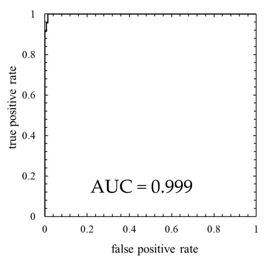
Figure 12. ROC curve of the model in which the number of mixture components K was 128 (threshold is 100th percentile’s value).

Next, Figure 13 shows the training data of this model. Note that the layout and the types of plots of the Figure 13 are the same as in the training data of the other models.

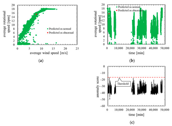
Figure 13. Training data of the model in which the number of mixture components K was 128 (threshold is 100th percentile’s value): (a) wind speed rotational speed characteristic; (b) time characteristics of rotational speed; (c) time characteristics of anomaly score.

As is clear from Figure 11, anomaly score increases immediately after the lightning strike and exceeds the threshold. Consequently, the data immediately after the lightning strike are properly detected as abnormal. Additionally, as shown in ROC curve of Figure 12, AUC is more than 0.99, indicating that anomaly detection was performed appropriately. Table 6 indicates that only four false negatives occurred. These four data are due to the time delay of anomaly detection. As shown in training data of Figure 13, the anomaly score during normal operation is stable and there is no sharp rise like immediately after a lightning strike, and hence, it is considered that the false positives are unlikely to occur.

3.4. The Model in Which the Number of Mixture Components K Was 256

This model performed anomaly detection with K set to 256. The 100th percentile’s value for the anomaly score calculated from the data during normal operation was used as the threshold.

Figure 14 shows the assessment result of this model. Note that, the layout and the types of plots of the Figure 14 are the same as in the assessment result of the other models.

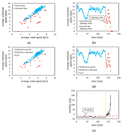
Figure 14. True label and assessment result of the model in which the number of mixture components K was 256 (threshold is 100th percentile’s value): (a) wind speed rotational speed characteristic with true label; (b) time characteristics of rotational speed with true label; (c) wind speed rotational speed characteristic with predicted label; (d) time characteristics of rotational speed with predicted label; (e) time characteristics of anomaly score.

This result is assessed by the confusion matrix and the ROC curve. Table 7 shows the confusion matrix, and Figure 15 shows the ROC curve.

Table 7. Confusion matrix of the model in which the number of mixture components K was 256 (threshold is 100th percentile’s value).

		Predicted
		Abnormal	Normal
True	Abnormal	21	2
	Normal	2	133

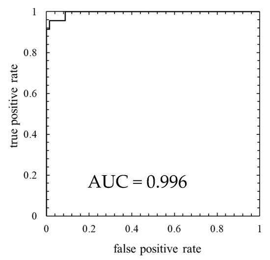
Figure 15. ROC curve of the model in which the number of mixture components K was 256 (threshold is 100th percentile’s value).

Next, Figure 16 shows the training data of this model. Note that, the layout and the types of plots of the Figure 16 are the same as in the training data of the other models.

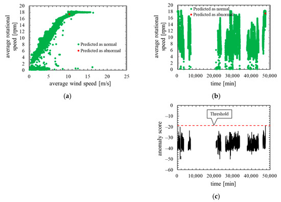
Figure 16. Training data of the model in which the number of mixture components K was 256 (threshold is 100th percentile’s value): (a) wind speed rotational speed characteristic; (b) time characteristics of rotational speed; (c) time characteristics of anomaly score.

As is clear from Figure 14, anomaly score increases immediately after the lightning strike and exceeds the threshold. Consequently, the data immediately after the lightning strike are properly detected as abnormal. However, the anomaly score exceeded the threshold before the lightning so that a false positive occurred. As shown by the ROC curve of Figure 15, AUC is more than 0.99, indicating that anomaly detection was performed appropriately. Additionally, Table 7 indicates that two false negatives and two false positives occurred. Furthermore, as shown in training data of Figure 16, the anomaly score during normal operation is stable and there is no sharp rise like immediately after a lightning strike. The false positives occur in the assessment data but the anomaly score of the training data is stable. Therefore, the model overfits the training data and most likely is not robust for unknown data.

4. Discussion

In this section, we compare anomaly detection accuracy of each model based on the results of Section 3 and examine improvement of accuracy. Since the threshold differs for each model, the comparison is performed based on the AUC of the ROC curve, which is an assessment method that does not depend on the threshold.

Table 8 summarizes AUC of each model.

Table 8. AUC of each model.

Model	AUC
K based on BIC (K = 29)	0.989
K = 64	0.994
K = 128	0.999
K = 256	0.996

As is clear as Table 8, AUC of the model with K = 128 is the highest, and it can be seen that it is the optimum model. Nevertheless, the model with K based on BIC selected 29 as K. Therefore, it became clear that the BIC does not decrease even with the optimum model for anomaly detection.

As shown in the AUC of the model with K = 256, it is considered that the anomaly detection accuracy does not improve by simply increasing K. The GMM will approximate predicted model in more detail if K is large, whereas the anomaly score of unknown data will increase because the model depends on training data. It is considered that this overfitting lowered the AUC of the model with K = 256.

From the above consideration, it can be seen that the method of automatically selecting K based on BIC used in normal GMMs is not effective for anomaly detection methods. If GMM is used as the anomaly detection method, the anomaly detection accuracy can be improved by setting K appropriately by comparing the accuracy and selecting the optimal model.

It became clear that a model with sufficient anomaly detection accuracy can be constructed using at least one month’s worth of training data. In this study, normal data for about 33 days were used as the training data, and, as shown in Table 8, high anomaly detection accuracy was confirmed in all models.

5. Conclusions

In this study, we constructed a lightning damage detection model for wind turbine blades using GMM based on SCADA data, and examined the method to improve the anomaly detection accuracy of the model. Wind speed and rotational speed were selected as features based on a previous study. Moreover, 0-1 standardization and moving average were performed as preprocessing. There are two methods for selecting hyperparameter K of GMM: one is automatic selection based on BIC and the other is manual selection of appropriate values. Anomaly detection with these two methods was performed and the accuracy was compared. As a result, it becomes clear that the model manually selected at K = 128 had the highest AUC and was the most suitable model. Hence, it was clarified that the performance of the model can be improved by using the method of manually selecting multiple K and selecting the model with the highest anomaly detection accuracy.

References

- Takada, Y. Wind Farm and Lightning: The Influence and Measures; Seizandou Shoten: Tokyo, Japan, 2015; pp. 72–84. [Google Scholar]
- Lightning risk management technology research committee for wind power generation systems. In Recent Trends Suggestions Lightning Risk Manage Wind Power System; Technical Report for the Institute of Electrical Engineers of Japan Number 1422; IEEJ Electronic Library: Tokyo, Japan, 2019; pp. 4–8.
- Ministry of Economy, Trade and Industry. New Energy Power Generation Facility Accident Response and Structural Strength Working Group. Available online: https://www.meti.go.jp/shingikai/sankoshin/hoan_shohi/denryoku_anzen/newenergy_hatsuden_wg/index.html (accessed on 20 December 2021).
- Kose, M.; Tanaka, S.; Yamamoto, K.; Sekioka, S.; Baba, Y.; Nagaoka, N. Effective Length of Counterpoises Connected to Wind Turbine Foundation. IEEE Trans. Power Deliv. 2021, 36, 3956–3963. [Google Scholar] [CrossRef]
- Triruttanapiruk, N.; Yamamoto, K.; Sumi, S.; Yokoyama, S.; Obayashi, K. Practical Use of Detection Techniques for Down Conductor Disconnections in Wind Turbine Blades. Electr. Power Syst. Res. 2020, 187, 106516. [Google Scholar] [CrossRef]
- Yamamoto, K.; Honjyo, N.; Yokoyama, S.; Yasuda, Y.; Sekioka, S.; Yamabuki, K. Technologies Developed to Operate Wind Turbines Reliably and Safely in a Lightning-Prone Environment; CIGRE Session 2020, C4-319; CIGRE: Ishikawa, Japan, 2020. [Google Scholar]
- Alipio, R.; de Barros, M.T.C.; Schroeder, M.A.O.; Yamamoto, K. Analysis of the Lightning Impulse and Low-frequency Performance of Wind Farm Grounding Systems. Electr. Power Syst. Res. 2020, 180, 106068. [Google Scholar] [CrossRef]
- Piantini, A. Lightning Interaction with Power Systems (Energy Engineering); IET (The Institution of Engineering and Technology): Stevenage, UK, 2020; ISBN 978-1785613913. [Google Scholar]
- Yamamoto, K.; Honjyo, N. Latest trends in technologies for sound operation of wind turbines against lightning. Electr. Eng. Jpn. 2018, 205, 3–7. [Google Scholar] [CrossRef]
- Ministry of Economy. Trade and Industry, Rules to Revise Part of Interpretation of Technical Standards for Wind Power Generation Facilities. Available online: https://www.meti.go.jp/policy/safety_security/industrial_safety/law/files/fuugikaishakukaisetsu.pdf (accessed on 20 December 2021).
- Hiroaki, K.; Kazuo, Y.; Shin’ichi, S. Influence of Lightning Detections and Damages on Availability of Wind Turbine Generation Systems; HV19076; The Institute of Electrical Engineers of Japan: Tokyo, Japan, 2019. [Google Scholar]
- Yamamoto, K.; Kashima, N.; Ueda, T.; Baba, S.; Sasaki, H.; Kanai, D. Noncontact Method to Diagnose Down-Conductor Disconnections in a Wind Turbine Blade Using X-ray Apparatuses; The Papers of Technical Meeting on High Voltage Engineering, IEE Japan, HV-17-26; Electric Institute: Tokyo, Japan, 2017; pp. 29–34. [Google Scholar]
- Eologix, Ice Detection and Temperature Measurement on Rotor Blades of Wind Turbines. Available online: https://www.eologix.com/en/solutions/windenergy/ (accessed on 20 December 2021).
- Yasuda, A.; Ogata, J.; Furusawa, Y.; Narusue, Y.; Murakawa, M.; Morikawa, H.; Iida, M. Wind Turbine Degradation Assessment Based on Condition Monitoring Model. Jpn. Wind Energy Assoc. 2018, 42, 53–62. [Google Scholar] [CrossRef]
- Pandit, R.K.; Infield, D. SCADA Based Wind Turbine Anomaly Detection Using Gaussian Process (GP) Models for Wind Turbine Condition Monitoring Purposes; IET (The Institution of Engineering and Technology): Stevenage, UK, 2018. [Google Scholar] [CrossRef] [Green Version]
- Cui, Y.; Bangalore, P.; Tjernberg, L.B. An Anomaly Detection Approach Based on Machine Learning and SCADA Data for Condition Monitoring of Wind Turbines. IET Renew. Power Gener. 2018, 12, 1249–1255. [Google Scholar] [CrossRef]
- Matsui, T.; Yamamoto, K.; Sumi, S.; Triruttanapiruk, N. Detection of lightning damage on wind turbine blades using the SCADA system. IEEE Trans. Power Deliv. 2021, 36, 777–784. [Google Scholar] [CrossRef]
- Svensén, M.; Bishop, C.M. Pattern Recognition and Machine Learning; Springer: Berlin/Heidelberg, Germany, 2007. [Google Scholar]
- Fraley, C.; Raftery, A.E. How many clusters? Which clustering method? Answers via model-based cluster analysis. Comput. J. 1998, 41, 578–588. [Google Scholar] [CrossRef]
- Hirai, Y. The First Pattern Recognition; Morikita: Tokyo, Japan, 2012; pp. 30–35. [Google Scholar]
Publisher’s Note: MDPI stays neutral with regard to jurisdictional claims in published maps and institutional affiliations. |
© 2021 by the authors. Licensee MDPI, Basel, Switzerland. This article is an open access article distributed under the terms and conditions of the Creative Commons Attribution (CC BY) license (https://creativecommons.org/licenses/by/4.0/).