
Dynamic Friction-Slip Model Based on Contact Theory
1
Centre of Ultra-Precision Optoelectronic Instrument Engineering, Harbin Institute of Technology, Harbin 150080, China
2
Key Lab of Ultra-Precision Intelligent Instrumentation, Harbin Institute of Technology, Ministry of Industry and Information Technology, Harbin 150080, China
*
Author to whom correspondence should be addressed.
Machines 2022, 10(10), 951; https://doi.org/10.3390/machines10100951
Submission received: 20 September 2022
/
Revised: 12 October 2022
/
Accepted: 14 October 2022
/
Published: 19 October 2022
(This article belongs to the Section Friction and Tribology)
Abstract
:In ultra-precision positioning equipment, the positioning accuracy is affected by the friction characteristics, especially the pre-slip stage. At present, the research on friction mainly includes contact theory and the dynamic friction process. There is no time variable in contact theory models, so they only apply to the stage of static contact, while the establishment of a friction dynamics model depends on parameter identification and cannot reflect the influence of a rough morphology and load. Therefore, neither theory can elucidate the ultra-precise slip mechanism. In this paper, maximum static friction force, tangential stiffness, and tangential damping models of contact surfaces were deduced through fractal contact theory. By substituting the contact parameters into the modified LuGre model, a dynamic slip model of the mask was established. Finally, the above model was verified by a reticle dynamic slip measurement system. The experimental results showed that in the pre-slip stage of the reticle, with an increase in the normal external load, the slippage of the reticle decreased. The theoretical value calculated by the model was basically consistent with the experimental value, and the slippage of the reticle mainly originated from the tangential deformation and relative sliding of the contact surface. With the increase in the normal external load, the proportion of the tangential deformation in the sliding of the entire contact surface was larger. For the change in slippage during different motion stages, the theoretical value was close to the experimental value after eliminating system errors such as vibration and fiber bending, which proved the correctness of the model in this paper.
1. Introduction
In the field of ultra-precision engineering, contact and friction between mechanical components are widespread. When a friction pair is subjected to tangential load, the contacting surfaces slide relative to one another, which affects the performance of the equipment. In lithography, in order to accurately project the pattern of a reticle onto a wafer, a reticle stage carries the reticle in a reciprocating motion, and the contact between the reticle and the stage is realized by vacuum adsorption. When the acceleration of the stage exceeds a certain value, there is significant relative slippage between the reticle and the chuck, which substantially affects the overlay accuracy of the lithography. In order to avoid the excessive deformation of the reticle, the adsorption force of the chuck should be smaller. Therefore, it is necessary to predict the slippage of the reticle from the point of view of the contact mechanism and suppress its sliding. The friction process has become a major problem in the ultra-precision positioning process due to its nonlinearity and uncertainty. In the research on the friction phenomenon, two types of friction models have been developed: a theoretical friction model for the friction mechanism and an empirical model for the dynamic friction process.
In the study of friction mechanisms, a contact friction model of a single asperity on the surface is usually established based on contact theory, and then the friction characteristics are extended to the entire surface based on a topographic characterization model. Aiming at a contact model of a single asperity, Hertz [1] constructed an accurate model of the contact area between the normal load and the elastic asperity; subsequently, the Johnson–Kendall–Robert (JKR) [2], Derjaguin–Muller–Toporov (DMT) [3], and Maguis–Dugdale (MD) [4,5] models introduced the Lennard–Jones potential [6] function to the Hertz model, and the adhesion model of contact asperities was established. Based on the finite element method, the Kogut–Etsion (KE) [7,8] model divided the deformation of the asperities into four stages, fully elastic, first elastic–plastic, second elastic–plastic, and fully plastic, which further improved the contact model. There are two main methods for the characterization of rough surfaces: the statistical approach represented by the Greenwood and Williamson (GW) [9] model, and the fractal theory put forward by Mandelbrot [10,11]. However, the characterization of rough surfaces by the GW model depends on the sampling length of the measurement. Fractal theory can realize the unique characterization of rough surfaces by determining the fractal dimension D and fractal roughness coefficient G. In recent years, theoretical models of contact stiffness [12,13,14], damping [15,16,17], contact area [18], static friction [19,20,21,22,23], etc., have been developed based on contact theory and fractal theory. The establishment of the theoretical friction model was based on the actual physical parameters. However, the above models do not include differential equations related to time. Therefore, the theoretical friction model can only describe the mechanism of static contact friction. When two contact surfaces slide relative to each other and produce dynamic friction, the above models are no longer applicable.
In the study of friction processes, numerous friction properties have been found, such as pre-slip [24], friction hysteresis [25], friction memory [26], and directional friction [27]. Ultra-precision equipment requires high positioning accuracy, so these friction characteristics need to be considered, especially pre-slip. The Coulomb model [28] was the first proposed friction model, which introduced the concept of the friction coefficient. On the basis of the Coulomb model, the nonlinearity in the friction process was characterized by the Stribeck model [29], which showed the relationship between the friction force and speed and found that in the low-speed region, the friction force decreases with an increase in speed. Dahl [24] simulated the pre-slip and hysteresis effects of friction for the first time by introducing differential equations. The bristle model [30] abstracted the friction resistance into the contact deformation resistance of elastic bristles. C. Canudas De Wit et al. [31] further divided the friction force into three parts (the bristle deformation resistance, the damping force generated by the bristle deformation speed, and the viscous damping force) and combined these with the Stribeck curve to propose a more complete model, the LuGre model. Subsequently, more dynamic friction models were proposed, including the elastic–plastic model [32], the Leuven model [33], and the GMS model [34]. The LuGre model not only accurately simulates friction behavior, but also has certain physical significance, so it is a very popular friction model. The above models are dedicated to accurately expressing various characteristics in the friction process for friction compensation in combination with control algorithms, so they are widely used in the field of control engineering [35,36,37,38], but they greatly simplify the contact of the contact surface. In addition, the above models are mostly used for friction compensation, and the parameters in the models (maximum static friction, tangential stiffness, tangential damping, etc.) are obtained through parameter identification. Therefore, the numerical values do not represent the real contact state, nor can they be used to study the influence of a rough morphology and contact load on slippage. In essence, they are empirical models and cannot provide guidance for the design of subsequent contact surfaces.
There are differences between theoretical models and empirical models for friction problems, so they have different application ranges. The mechanism of friction and slip cannot be fully explained by theoretical models or empirical models alone. The dynamic friction characteristics of two objects mainly depend on three important parameters: the maximum static friction, tangential stiffness (the elastic deformation of the contact surface under tangential load), and tangential damping (the energy dissipation of the contact surface during sliding) of the contact surface, and the above parameters mainly depend on the roughness and the contact states.
In Section 1, the current mainstream contact theory model and friction dynamics model are introduced. In Section 2, based on fractal theory and contact theory, the maximum static friction force model of the contact surface is established. In Section 3, the contact deformation of a single asperity under a normal load and tangential load is analyzed. Considering fractal theory, tangential stiffness and damping models of the contact surface are established. In Section 4, taking account of the dry friction between the reticle and the chuck in lithography, the LuGre model is modified, and the dynamic slip model is established. Section 5 shows the dynamic slip measurement system, which measures the slip of the reticle under different vacuum degrees (normal load). The experimental results showed that in the pre-sliding stage, the slippage between the reticle and the chuck mainly originated from the deformation of the contact surface; with an increase in the normal load, the slippage of the reticle decreased, and the theoretical value fit well with the experimental value, which confirmed the correctness of the dynamic slip mode in this paper.
2. Maximum Static Friction Model
Thomas pointed out that most engineering rough surfaces have obvious fractal characteristics [39]. According to the Yan–Komvopoulos (YK) model [40], the anisotropic fractal function can be expressed as a function of a single variable:
where Z represents the profile height of the surface; L is the sample length; G is the fractal roughness coefficient; D denotes the fractal dimension of the surface; γ is a parameter that determines the density of frequencies in the surface and is a constant greater than 1, because the height of most rough surface profiles obeys a normal distribution—in order to reflect this feature, γ usually takes a value of 1.5; M represents the number of overlapping ridges on the fractal surface; is the random phase; and n is the frequency index.
The contact between two rough surfaces is equivalent to the contact between the rough surface and the ideal rigid plane [9]. When a single asperity is in contact with a rigid plane and bears a normal load Pn, since the actual contact size of the asperity is much smaller than its radius of curvature, the asperity can be approximately regarded as a sphere, as shown in Figure 1.
In Figure 1, r’ is the truncated radius of the asperity. Based on the YK model, the deformation of the asperity is:
The radius of the curvature of the asperity can be obtained as follows:
where a’ is the truncated contact area of the asperity, .
According to the Hertz theory, when the deformation is less than the critical elastic deformation δec, the asperity deforms elastically, and the elastic critical deformation can be expressed as:
where E is the equivalent elastic modulus of the rough contact surface, expressed as: (E1, E2 and , are the elastic modulus and Poisson’s ratio of the two contact surface materials, respectively). H is the hardness of the softer material; K represents the hardness coefficient; and the relationship between K and the Poisson’s ratio v of the material is: .
According to Equations (2) and (4), the elastic critical truncated area of asperities can be obtained as follows:
On the basis of the Hertz theory and according to the expansion law of the plastic deformation of an asperity, the deformation of the asperity could be divided into four stages: fully elastic (), first elastic–plastic (), second elastic–plastic (), and fully plastic (). Based on Equations (2) and (4), the fractal theory divides the deformation into four stages according to the critical truncated area, as shown in Figure 2.
and are the elastic–plastic and plastic critical truncated areas, respectively, which can be expressed as:
When the contact truncated area satisfies , the asperity deforms elastically, and the normal contact load of a single asperity can be expressed as:
In addition, according to finite element analysis and data fitting, Kogut and Etsion [7] presented the relationship between the normal load, the real contact area, and the deformation of the asperities in first elastic–plastic and second elastic–plastic deformation stages as follows:
When the deformation of the asperity is in the stage of the fully plastic regime, its truncated area satisfies , and the relationship between the normal load and the truncated area of the asperity is:
When the normal load acts on the contact surface, the asperities in the second elastic–plastic and fully plastic regime undergo plastic flow under the local load and can no longer bear the tangential load. Based on the Hamilton theory [41] and the Tresca yield condition, the expressions of the maximum static friction force of a single asperity in the fully elastic region and the elastic–plastic region are as follows:
where is the shear strength of the contact surface material.
Mandelbrot [10,11] compared the contact conditions of the asperities on a fractal rough surface to the distribution of islands on the Earth, believing that the distribution of the truncated contact area a’ of the asperities resembles the distribution of islands in the ocean; thus, he proposed the following truncated contact area density distribution function for the asperities:
where is the maximum truncated contact area.
The maximum static friction force of the contact surfaces is the integral of the tangential load of the asperity in the fully elastic and the first elastic–plastic regime, which can be expressed as:
where Tep1 is the maximum static friction force of the asperity in the first elastic–plastic regime, and Te represents the maximum static friction force of the asperity in the fully elastic deformation stage.
3. Tangential Stiffness and Damping Models
When the asperities are subjected to normal load, the deformation is divided into four stages. When the force is unloaded, the asperities in the fully plastic regime cannot return to their original shape, and only energy dissipation occurs. After unloading the normal force, the deformation of the asperities in the first and second elastic–plastic regions cannot be completely restored. At this time, the asperities both store and dissipate energy. The deformation process of the elastically deformed asperities is completely reversible, and after unloading the normal force, only energy storage occurs. The amount of energy stored depends on the stiffness of the interface, while the amount of energy dissipated depends on the damping of the interface. Therefore, when studying the tangential stiffness of a contact surface, it is necessary to consider the asperities in the fully elastic, first elastic–plastic, and second elastic–plastic regimes.
A single asperity produces a circular contact area under the action of normal load ; the normal stress at the boundary of the contact circle is small, while the shear stress tends to infinity. A tangential load of any magnitude will cause the asperity to slip in the contact circle boundary. When the tangential load is less than the maximum static friction force, the contact surface is divided into an annular slip area and a non-slip area (adhesion area), and the asperities appear to slip locally, as shown in Figure 3. A narrow slip ring corresponds to a small tangential load, and as the tangential load increases, the slip ring becomes wider. When the tangential load reaches the maximum static friction force, the contact surface is completely occupied by the slip area, and the entire asperity begins to slip tangentially.
When two rough surfaces are in contact and bear a tangential load, the asperity will slide locally, and the tangential load and tangential displacement of a single asperity have the following relationship [42]:
where is the equivalent shear modulus of the contact surface, which satisfies the relation ; and is the friction coefficient of the contact surface.
In this study, the ratio of the tangential load to the normal load for a single asperity is equivalent to the ratio of the tangential load to the normal load for the entire contact surface, that is, . Thus, the tangential stiffness of a single asperity in contact can be obtained:
The total tangential stiffness of the contact surfaces can be obtained as:
where kτep2 is the tangential stiffness of the asperity in the second elastic–plastic regime, kτep1 is the tangential stiffness of the asperity in the first elastic–plastic regime, and kτe represents the tangential stiffness of the asperity in the fully elastic deformation stage.
When contact surfaces are subjected to both normal load and tangential alternating load, and the tangential load does not exceed the maximum static friction force, the asperity presents a slip ring, as shown in Figure 3, and the tangential displacement and load of the asperity form a closed elliptic curve, as shown in Figure 4. The energy dissipation in one loading cycle is equal to the area of the closed curve formed by the displacement and the load.
The energy dissipation of the contact surface occurs in the plastic deformation stage, so the damping model mainly considers the asperities in the first elastic–plastic regime and the second elastic–plastic regime. The elastically deformed asperities only store energy, and the energy is released after the tangential force is unloaded. Therefore, the energy storage involves asperities of the fully elastic regime, first elastic–plastic regime, and second elastic–plastic regime.
In one cycle of tangential alternating load, the tangential damping energy consumption of a single asperity is expressed as [42]:
The total energy dissipation on the contact surface is the synthesis of the energy dissipation of all asperities. The energy dissipation of all asperities in the first and second elastic–plastic regime on the contact surface is as follows:
where wdep1 is the energy dissipation of the asperity in the first elastic–plastic regime, and wdep2 is the energy dissipation of the asperity in the second elastic–plastic regime.
In one cycle of the tangential excitation force, the maximum energy required for the tangential displacement of a single asperity is the integral of the tangential load with respect to the tangential displacement, which can be written as:
The energy storage of the contact surface is the sum of the energy storage of all asperities in the fully elastic region, the first elastic–plastic region, and the second elastic–plastic region, which can be written as:
where wte represent the energy storage of the asperity in the fully elastic regime, wtep1 is the energy storage of the asperity in the first elastic–plastic region, and wtep2 is the energy storage of the asperity in the second elastic–plastic regime,
According to the Sabot theory [43], the tangential damping of the rough contact surface can be obtained by the following formula:
where m is the is the mass of the slider.
4. Dynamic Slip Model
The dynamic friction of a contact surface is characterized by nonlinearity and uncertainty, which is a major problem to be solved in the high-precision positioning of ultra-precision equipment. The relative sliding of the two contact surfaces can be divided into two stages: pre-slip and macro-slip. The LuGre model, as the most popular dynamic friction model, is derived from the bristle model, which regards the asperity on the rough surface as a bristle with a certain stiffness. When there is a relative velocity between the two surfaces, the bristle deforms and generates resistance, as shown in Figure 5.
In the pre-slip stage, there are two sources of friction, the elastic resistance generated by the deformation of the bristles and the damping force created during the deformation of the bristles, and the relative displacement is reflected in the deformation of the bristles. When the deformation of the bristles reaches the maximum, macro-slip appears between the contact surfaces, the deformation of the bristles remains at the maximum value, and the friction force obeys the Stribeck curve. During this process, the frictional force changes depending on the relative velocity, damping, and viscosity of the contact surfaces. The LuGre model is shown in Equation (25) [31]:
where z is the equivalent deformation of the bristles; is the equivalent stiffness of all bristles on the contact surface; is the equivalent damping of all bristles on the contact surface; is the deformation speed of the bristles; represents the coefficient of viscosity of all bristles on the contact surface; is the relative sliding velocity of the contact surfaces; and is the friction force based on the Stribeck curve.
In lithography, the reticle stage causes the reticle to move through vacuum adsorption; the driving force of the stage comes from a linear motor, and the reticle is driven by the friction force from the vacuum chuck. The friction force depends on the contact between the reticle and the chuck and the dynamic friction characteristics. The dynamic friction slip model of the reticle included two parts: (1) the dynamic model of the reticle and the stage and (2) the friction model of the contact surfaces. During the movement of the stage, the dynamic model of the reticle and the chuck is equivalent to a spring-damped vibrator model, as shown in the Figure 6. is the friction force between the contact surfaces, m1 is the quality of the stage, m2 is the quality of the reticle, is the equivalent stiffness of the contact surface, and is the equivalent damping of the contact surfaces.
The relative sliding between reticle and chuck represents dry friction, and there is no obvious displacement during the actual movement, so there was no need to consider the viscosity between the contact surfaces. In Equation (25), the equivalent stiffness could be replaced by the tangential stiffness , and the damping could be replaced by the tangential damping .
In the pre-slip stage, the tangential deformation of the contact surface is less than the maximum deformation, and as the relative sliding speed or sliding distance increases, the friction process reaches a macro-slip state. In this case, the tangential deformation of the contact surface remains at the maximum value, the change in friction depends on the change in damping force, and the maximum tangential deformation of the contact surface could be expressed as:
In the pre-slip stage, the Stribeck friction is approximately equal to the maximum static friction of the contact surface, that is, . Therefore, the slip model of the reticle could be expressed as:
where is the slippage of the reticle relative to the chuck and is the acceleration of the reticle stage.
5. Experiment
5.1. Surface Morphology Measurement
In lithography, the reticle is fixed on the reticle stage by a pair of vacuum chucks. In order to simulate the actual working conditions of lithography, a pair of fused silica chucks with nano-roughness were processed and combined with a 6-inch standard reticle to form a friction pair. The material of the reticle was quartz ceramic, and the roughness of its contact surface (Ra) was <1 nm. The reticle surface and the chuck adsorption surface were scanned and measured with a three-dimensional profiler. The sampling spacing was 0.8 μm, the sampling length was 1 mm, and the contact surfaces are shown in Figure 7.
According to the measurements, the surface roughness of the chuck (Ra) was 1.50 nm, and the surface roughness of the reticle was 1.22 nm. When two surfaces come into contact, the equivalent surface can be replaced by the difference between them. In this paper, the fractal dimension D of the equivalent surface was determined based on the 3D-RMS method [44]. D determined the details of the surface, and the roughness parameter G determined the height of a single asperity on the surface. Therefore, after determining D, the roughness coefficient of the contact surface was calculated based on the roughness. The fractal dimension and roughness coefficient of the chuck, reticle, and equivalent surface are shown in Table 1.
5.2. Slip Measurement
The reticle stage drives the reticle to complete a reciprocating motion. During the acceleration and deceleration of the stage, the reticle slides. In order to measure the sliding of the reticle during movement, a dynamic slip measurement system was designed, as shown in Figure 8. The system included a reticle, vacuum chuck, vacuum system, linear stage with air bearings, and laser interferometer. The maximum vacuum produced by the vacuum system was 80 kPa. The displacement resolution of the laser interferometer was 0.4 nm. In order to reduce the influence of external noise on the experimental system, a sound-proofing mechanism was also designed.
The area of the adsorption surface of the chuck was 909 mm2. The nominal contact area was 2101.72 mm2. When the reticle was in contact with the chuck, the normal external load F included the gravity of the reticle and the pressure generated by the vacuum, which could be expressed as:
where Av is the area of the adsorption surface, Pv represents the vacuum degree, and Gr is the gravity of the reticle.
The size of the reticle was 152. 4 mm × 152.4 mm × 6.34 mm, with a mass of 0.321 kg. The material parameters [45,46] of the reticle and chuck are shown in Table 2.
Based on the model described in Section 2, Section 3 and Section 4, the maximum static friction, tangential stiffness, tangential damping, and maximum tangential deformation between the reticle and chuck were obtained for chuck vacuum degrees of 0.6 kPa, 2 kPa, 4 kPa, 7 kPa, 10 kPa, and 20 kPa, as shown in Table 3.
In lithography, the motion process of the reticle stage in a single cycle is as follows: static–acceleration phase–uniform motion phase–deceleration phase–static. The greater the acceleration of the stage, the greater the friction required by the reticle to ensure synchronous movement. In the experiment, the maximum speed of the positioning stage was set to be 0.5 m/s, and the maximum acceleration was 1 m/s2, as shown in Figure 9.
The theoretical slip and deformation of the contact surfaces could be obtained by substituting the parameters in Table 3 and the acceleration curve into Equation (27). Figure 10 shows the comparison of the theoretical deformation and slippage and the measured slippage of the contact surface under different vacuum degrees. It can be seen from Figure 10 that with the increase in the normal external load, the slip of the reticle showed a decreasing trend; the slippage did not exceed the maximum deformation of the contact surfaces; and the friction was in the pre-slip stage. In a reciprocating motion cycle, the variation trend of the theoretical slip with time was basically consistent with the experimental value.
When the reticle stage reached the steady acceleration phase (0.25 s~0.6 s) from static (0.0 s), we measured the average slippage between the reticle and the chuck for suction-cup vacuum degrees of 0.6 kPa, 2 kPa, 4 kPa, 7 kPa, 10 kPa, and 20 kPa, as shown in Table 4. In this state, the reticle demonstrated a forward slip, and the average error between the theoretical value and the experimental value of the slippage was 2.93%~27.72%.
Table 5 shows the average slippage between the reticle and the chuck under different vacuum degrees from the stable acceleration phase (0.25 s~0.6 s) to the uniform motion phase (0.73 s~1.5 s) of the reticle stage. At this time, the acceleration dropped to 0 m/s2, the deformation between the reticle and the chuck started to recover, and the slippage decreased. The average error between the theoretical value and the experimental value of slippage was 2.88~404.26%. When the true space was 20 kPa, the maximum error was 404.26%, which was due to the deformation of the optical fiber of the laser interferometer, resulting in an insufficient slippage change (0.47 nm) for the reticle from the stable acceleration phase to the uniform movement phase of the reticle stage. In addition, when the vacuum degree was 0.6 kPa, the error between the theoretical slippage and the experimental value was 55.81%, due to the relative displacement between the reticle and the chuck.
When the reticle stage moved from the uniform motion phase (0.73 s~1.5 s) to the stable deceleration phase (1.65 s~2.0 s), we measured the average slippage and error of the reticle under different chuck vacuum degrees, as shown in Table 6. In this process, the acceleration of the reticle stage was negative, and the reticle demonstrated a reverse slip. The average error between the theoretical value of slippage and the experimental value was 6.44~21.78%.
Table 7 shows the average slippage and error of the reticle under different vacuum degrees from the stable deceleration phase (1.65 s~2.0 s) to static (2.3 s). At this time, the acceleration of the reticle stage decreased, and the deformation between the reticle and the chuck began to recover. The average error between the theoretical value and the experimental value of the slippage was 12.21%~51.46%. When the vacuum degree was 0.6 kPa, the normal load between the reticle and the chuck was too small, and there was a relative displacement between the contact surfaces, resulting in a large difference between the theoretical slippage and the experimental value.
In addition, it can be seen from Figure 10 that the slippage between the reticle and the chuck included the deformation and relative displacement of the contact surfaces. When the vacuum degree was larger, the proportion of contact surface deformation in the slippage was larger. This was mainly because the tangential stiffness of the contact surfaces increased with the increase in normal load.
6. Conclusions
The friction-slip process between contact surfaces is divided into the pre-slip and macro-slip. In ultra-precision equipment, the positioning accuracy is affected by the friction characteristics, especially the pre-slip. The main factors influencing the pre-slip are the maximum static friction force, tangential stiffness, and tangential damping; the maximum static friction force and tangential stiffness together determine the critical state of the contact surface transitioning to macroscopic sliding. Based on contact theory, maximum static friction, tangential stiffness, and tangential damping models of a contact surface were established in this paper. Then, by modifying the LuGre model and introducing the above contact model, a dynamic slip model was established.
In order to verify the accuracy of the dynamic slippage model based on contact theory, we built a dynamic slippage measurement system by simulating the contact and movement process between a lithographic reticle and chuck. The experimental results showed that when the vacuum degree of the chuck was 0.6 kPa, 2 kPa, 4 kPa, 7 kPa, 10 kPa, or 20 kPa, and the acceleration of the stage formed a trapezoidal wave with a maximum value of 1 m/s2, there was a pre-sliding phenomenon between the reticle and the chuck. It was found from the measurement results that with the increase in normal load, the slippage of the reticle decreased, and the theoretical value was consistent with the experimental value. When the movement process of the reticle stage changed, the overall error between the theoretical slip of the reticle and the experimental value was small; when the vacuum degree was 2 kPa, 4 kPa, 7 kPa, or 10 kPa, the error between the theoretical slippage and the experimental value was less than 30%. However, the relative displacement between the contact surfaces caused errors. When the vacuum degree was 0.6 kPa, due to the obvious relative displacement between the reticle and the chuck, the error between the theoretical slippage and the experimentally measured slip was large, and the maximum value was not more than 60%. In addition, when the vacuum degree was 20 kPa, the slippage measured in the experiment was too small due to the bending of the optical fiber of the laser interferometer from the stable acceleration phase to the uniform motion phase of the reticle stage, which led to a large error between the theoretical value and the experimental value.
Author Contributions
Conceptualization, H.W.; data curation, H.W.; formal analysis, H.W.; funding acquisition, J.C. and J.W.; methodology, H.W.; project administration, J.C., J.W. and J.T.; resources, J.W.; software, H.W.; supervision, J.C., J.W. and J.T.; visualization, H.W. and J.C.; writing—original draft, H.W.; writing—review and editing, H.W. All authors have read and agreed to the published version of the manuscript.
Funding
This research was funded by the Outstanding Youth Project of the Natural Science Foundation of Heilongjiang Province (Grant JQ2019E002), the National Natural Science Foundation of China (Grant 52175499), and the National Major Science and Technology Projects of China (Grant No. 2017ZX02101006-005).
Institutional Review Board Statement
Not applicable.
Informed Consent Statement
Not applicable.
Data Availability Statement
The authors will provide data and material upon reasonable request.
Conflicts of Interest
The authors declare that they have no conflict of interest.
References
- Hertz, H. On the contact of elastic solids. J. Reine Angew. Math. 1881, 92, 156–171. [Google Scholar]
- Johnson, K.L.; Kendall, K.; Roberts, A.D. Surface energy and the contact of elastic solids. Proc. R. Soc. Lond. A Math. Phys. Sci. 1971, 324, 301–313. [Google Scholar]
- Derjaguin, B.V.; Muller, M.V.; Toporov, Y.P. Effect of contact deformations on the adhesion of particles. J. Colloid Interface Sci. 1975, 53, 314–326. [Google Scholar] [CrossRef]
- Maugis, D. Adhesion of spheres: The JKR-DMT transition using a dugdale model. J. Colloid Interface Sci. 1992, 150, 243–269. [Google Scholar] [CrossRef]
- Maugis, D. On the contact and adhesion of rough surfaces. J. Adhes. Sci. Technol. 1996, 10, 161–175. [Google Scholar] [CrossRef]
- Muller, V.; Yushchenko, V.; Derjaguin, B. On the influence of molecular forces on the deformation of an elastic sphere and its sticking to a rigid plane. Prog. Surf. Sci. 1994, 45, 157–167. [Google Scholar] [CrossRef]
- Kogut, L.; Etsion, I. Elastic-plastic contact analysis of a sphere and a rigid flat. J. Appl. Mech. 2002, 69, 657–662. [Google Scholar] [CrossRef] [Green Version]
- Kogut, L.; Etsion, I. A static friction model for elastic-plastic contacting rough surfaces. J. Tribol. 2004, 126, 34–40. [Google Scholar] [CrossRef] [Green Version]
- Greenwood, J.A.; Williamson, J.B.P. Contact of nominally flat surfaces. Proc. R. Soc. Lond. Ser. A Math. Phys. Sci. 1966, 295, 300–319. [Google Scholar]
- Mandelbrot, B.B. Stochastic models for the Earth’s relief, the shape and the fractal dimension of the coastlines and the number-area rule for islands. Proc. Natl. Acad. Sci. USA 1975, 72, 3825. [Google Scholar] [CrossRef] [PubMed] [Green Version]
- Mandelbrot, B.B. The Fractal Geometry of Nature; W.H. Freeman: New York, NY, USA, 1982. [Google Scholar]
- Pohrt, R.; Popov, V.L. Normal Contact Stiffness of Elastic Solids with Fractal Rough Surfaces. Phys. Rev. Lett. 2012, 108, 104301. [Google Scholar] [CrossRef]
- Buczkowski, R.; Kleiber, M.; Starzynski, G. Normal contact stiffness of fractal rough surfaces. Arch. Mech. 2014, 66, 411–428. [Google Scholar]
- Liu, P.; Zhao, H.; Huang, K.; Chen, Q. Research on normal contact stiffness of rough surface considering friction based on fractal theory. Appl. Surf. Sci. 2015, 349, 43–48. [Google Scholar] [CrossRef]
- Zhang, X.; Wang, N.; Lan, G.; Wen, S.; Chen, Y. Tangential Damping and Its Dissipation Factor Models of Joint Interfaces Based on Fractal Theory with Simulations. J. Tribol. 2013, 136, 011704. [Google Scholar] [CrossRef]
- Zhao, Y.; Xu, J.; Cai, L.; Shi, W.; Liu, Z. Stiffness and damping model of bolted joint based on the modified three-dimensional fractal topography. Proc. Inst. Mech. Eng. Part C J. Mech. Eng. Sci. 2016, 231, 279–293. [Google Scholar] [CrossRef]
- Pan, W.; Li, H.; Qu, H.; Ling, L.; Wang, L. Investigation of Tangential Contact Damping of Rough Surfaces from the Perspective of Viscous Damping Mechanism. J. Tribol. 2020, 143, 041501. [Google Scholar] [CrossRef]
- Hanaor, D.A.H.; Gan, Y.; Einav, I. Contact mechanics of fractal surfaces by spline assisted discretisation. Int. J. Solids Struct. 2015, 59, 121–131. [Google Scholar] [CrossRef]
- Pan, W.; Li, X.; Wang, X. Contact mechanics of elastic-plastic fractal surfaces and static friction analysis of asperity scale. Eng. Comput. 2021, 38, 131–150. [Google Scholar] [CrossRef]
- Pan, W.; Li, X.; Wang, L.; Mu, J.; Yang, Z. A loading fractal prediction model developed for dry-friction rough joint surfaces considering elastic-plastic contact. Acta Mech. 2018, 229, 2149–2162. [Google Scholar] [CrossRef]
- Pan, W.; Yang, Z.; Sun, Z.; Li, X.; Guo, N. Three-dimensional fractal model of normal contact damping of dry-friction rough surface. Adv. Mech. Eng. 2017, 9, 1687814017692699. [Google Scholar] [CrossRef] [Green Version]
- Pan, W.; Li, X.; Wang, L.; Mu, J.; Yang, Z. Influence of surface topography on three-dimensional fractal model of sliding friction. AIP Adv. 2017, 7, 095321. [Google Scholar] [CrossRef] [Green Version]
- Janahmadov, A.K.; Javadov, M.Y. Synergetics and Fractals in Tribology; Springer International Publishing: Cham, Switzerland, 2016. [Google Scholar]
- Dahl, P.R. Solid Friction Damping of Mechanical Vibrations. AIAA J. 1976, 14, 1675–1682. [Google Scholar] [CrossRef]
- Awaddy, B.A.; Shih, W.-C.; Auslander, D.M. Nanometer positioning of a linear motion stage under static loads. IEEE/ASME Trans. Mechatron. 1998, 3, 113–119. [Google Scholar] [CrossRef]
- Armstrong-Hélouvry, B.; Dupont, P.; De Wit, C.C. A survey of models, analysis tools and compensation methods for the control of machines with friction. Automatica 1994, 30, 1083–1138. [Google Scholar] [CrossRef]
- Zmitrowicz, A. Models of kinematics dependent anisotropic and heterogeneous friction. Int. J. Solids Struct. 2006, 43, 4407–4451. [Google Scholar] [CrossRef] [Green Version]
- Mansour, W.; Filho, D.T. Impact dampers with coulomb friction. J. Sound Vib. 1974, 33, 247–265. [Google Scholar] [CrossRef]
- Jacobson, B. The Stribeck memorial lecture. Tribol. Int. 2003, 36, 781–789. [Google Scholar] [CrossRef]
- Haessig, D.A., Jr.; Friedland, B. On the Modeling and Simulation of Friction. J. Dyn. Syst. Meas. Control 1991, 113, 354–362. [Google Scholar] [CrossRef]
- De Wit, C.C.; Olsson, H.; Astrom, K.; Lischinsky, P. A new model for control of systems with friction. IEEE Trans. Autom. Control 1995, 40, 419–425. [Google Scholar] [CrossRef] [Green Version]
- Dupont, P.; Armstrong, B.; Hayward, V. Elasto-plastic friction model: Contact compliance and stiction. In Proceedings of the 2000 American Control Conference (ACC), Chicago, IL, USA, 28–30 June 2000. [Google Scholar]
- Swevers, J.; Al-Bender, F.; Ganseman, C.; Projogo, T. An integrated friction model structure with improved presliding behavior for accurate friction compensation. IEEE Trans. Autom. Control 2000, 45, 675–686. [Google Scholar] [CrossRef]
- Lampaert, V.; Al-Bender, F.; Swevers, J. A generalized Maxwell-slip friction model appropriate for control purposes. In Proceedings of the 2003 IEEE International Workshop on Workload Characterization, St. Petersburg, Russia, 20–22 August 2003. [Google Scholar]
- Bona, B.; Indri, M.; Smaldone, N. Rapid Prototyping of a Model-Based Control with Friction Compensation for a Direct-Drive Robot. IEEE/ASME Trans. Mechatron. 2006, 11, 576–584. [Google Scholar] [CrossRef]
- Minh, T.N.; Ohishi, K.; Takata, M.; Hashimoto, S.; Kosaka, K.; Kubota, H.; Ohmi, T. Adaptive Friction Compensation Design for Submicrometer Positioning of High Precision Stage. In Proceedings of the 2007 IEEE International Conference on Mechatronics, Kumamoto, Japan, 8–10 May 2007. [Google Scholar]
- Keck, A.; Zimmermann, J.; Sawodny, O. Friction parameter identification and compensation using the elastoplastic friction model. Mechatronics 2017, 47, 168–182. [Google Scholar] [CrossRef]
- Tran, X.B. Nonlinear Control of a Pneumatic Actuator Based on a Dynamic Friction Model. J. Mech. Eng. 2021, 67, 458–472. [Google Scholar]
- Thomas, A.P.; Thomas, T.R. Engineering Surface as Fractals, Fractal Aspects of Material; Materials Research Society: Pittsburgh, PA, USA, 1986. [Google Scholar]
- Yan, W.; Komvopoulos, K. Contact analysis of elastic-plastic fractal surfaces. J. Appl. Phys. 1998, 84, 3617–3624. [Google Scholar] [CrossRef]
- Hamilton, G.M. Explicit equations for the stresses beneath a sliding spherical contact. Proc. Inst. Mech. Eng. Part C J. Mech. Eng. Sci. 1983, 197, 53–59. [Google Scholar] [CrossRef]
- Johnson, K.L. Contact Mechanics; Cambridge University Press: Cambridge, UK, 1987. [Google Scholar]
- Sabot, J.; Krempf, P.; Janolin, C. Non-linear vibrations of a sphere-plane contact excited by a normal load. J. Sound Vib. 1998, 214, 359–375. [Google Scholar] [CrossRef]
- Zuo, X.; Zhu, H.; Zhou, Y.; Li, Y. A new method for calculating the fractal dimension of surface topography. Fractals 2015, 23, 1550022. [Google Scholar] [CrossRef]
- Naaijkens, G.-J.P. Reticle Side Wall Clamping. Ph.D. Thesis, Eindhoven University of Technology, Eindhoven, The Netherlands, 2013. [Google Scholar]
- Kingery, W.D.; Bowen, H.K.; Uhlmann, D.R. Introduction to Ceramics, 2nd ed.; John Wiley & Sons: Hoboken, NJ, USA, 1976. [Google Scholar]
Figure 1.
Contact and deformation of single asperity.

Figure 2.
Four stages of asperity deformation.

Figure 3.
Contact of asperity under tangential load.

Figure 4.
Relationship between tangential displacement and tangential load.
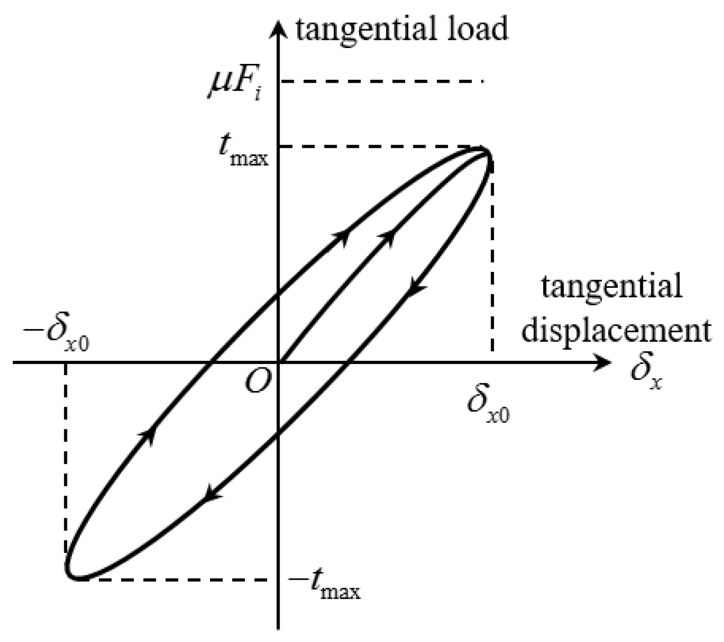
Figure 5.
Contact based on bristle model.

Figure 6.
Equivalent contact model for reticle and chuck.

Figure 7.
Reticle and chuck and their surface morphology. ① represents the fused quartz surface of the chuck, and ② represents the quartz ceramic surface of the reticle.
Figure 7.
Reticle and chuck and their surface morphology. ① represents the fused quartz surface of the chuck, and ② represents the quartz ceramic surface of the reticle.

Figure 8.
Dynamic friction sliding measurement system: (a) schematic of dynamic friction sliding measurement system; (b) dynamic friction sliding measurement experiment.
Figure 8.
Dynamic friction sliding measurement system: (a) schematic of dynamic friction sliding measurement system; (b) dynamic friction sliding measurement experiment.

Figure 9.
Acceleration of linear stage.

Figure 10.
Deformation of contact surfaces, theoretical slippage, and measured slippage for vacuum degrees of (a) 0.6 kPa; (b) 2 kPa; (c) 4 kPa; (d) 7 kPa; (e) 10 kPa; and (f) 20 kPa.
Figure 10.
Deformation of contact surfaces, theoretical slippage, and measured slippage for vacuum degrees of (a) 0.6 kPa; (b) 2 kPa; (c) 4 kPa; (d) 7 kPa; (e) 10 kPa; and (f) 20 kPa.


Table 1.
D and G confirmed by 3D-RMS method.
| Surface | D | G |
|---|---|---|
| Chuck | 2.9271 | 1.125 × 10⁻¹¹ m |
| Reticle | 2.7532 | 6.653 × 10⁻¹³ m |
| Equivalent surface | 2.8821 | 7.768 × 10⁻¹² m |
Table 2.
Reticle and chuck material parameters.
| Material | Quartz Ceramic | Fused Silica |
|---|---|---|
| Young’s modulus E (GPa) | 70.5 | 90.3 |
| Shear modulus G (GPa) | 30.2 | 36.3 |
| Hardness H (GPa) | 1.372 | 6.5 |
| (MPa) | 490 | 500 |
| Poisson’s ratio υ | 0.164 | 0.243 |
Table 3.
Contact parameters between reticle and chuck under different vacuum degrees.
| Vacuum Degree (kPa) | Normal External Load (N) | Maximum Static Friction (N) | Tangential Stiffness (N/m) | Tangential Damping (Ns/m) | Maximum Tangential Deformation (nm) |
|---|---|---|---|---|---|
| 0.6 | 3.6912 | 0.4868 | 1.4878 × 10⁷ | 771.0516 | 32.7295 |
| 2 | 4.9638 | 0.7372 | 2.1478 × 10⁷ | 708.8274 | 34.3235 |
| 4 | 6.7818 | 1.0861 | 3.0343 × 10⁷ | 712.2624 | 35.7941 |
| 7 | 9.5088 | 1.7201 | 4.5509 × 10⁷ | 749.7264 | 37.7969 |
| 10 | 12.2358 | 2.4402 | 6.1890 × 10⁷ | 799.5422 | 39.4280 |
| 20 | 21.3258 | 5.7685 | 1.3173 × 10⁸ | 994.1022 | 43.7903 |
Table 4.
Theoretical value, experimental value, and error of slippage (static to steady acceleration phase).
Table 4.
Theoretical value, experimental value, and error of slippage (static to steady acceleration phase).
| Vacuum Degree (kPa) | Theoretical Value of Slippage (nm) | Experimental Value of Slippage (nm) | Theoretical Error |
|---|---|---|---|
| 0.6 | 40.85 | 33.05 | 23.60% |
| 2 | 21.36 | 17.36 | 23.04% |
| 4 | 13.27 | 10.39 | 27.72% |
| 7 | 8.09 | 7.86 | 2.93% |
| 10 | 5.70 | 6.03 | 5.47% |
| 20 | 2.58 | 2.46 | 4.88% |
Table 5.
Theoretical value, experimental value, and error of slippage (stable acceleration phase to uniform motion phase).
Table 5.
Theoretical value, experimental value, and error of slippage (stable acceleration phase to uniform motion phase).
| Vacuum Degree (kPa) | Theoretical Value of Slippage (nm) | Experimental Value of Slippage (nm) | Theoretical Error |
|---|---|---|---|
| 0.6 | −10.00 | −22.63 | 55.81% |
| 2 | −10.04 | −11.17 | 10.12% |
| 4 | −8.30 | −8.75 | 5.14% |
| 7 | −6.08 | −6.26 | 2.88% |
| 10 | −4.56 | −4.06 | 12.32% |
| 20 | −2.37 | −0.47 | 404.26% |
Table 6.
Theoretical value, experimental value, and error of slippage (uniform motion phase to stable deceleration phase).
Table 6.
Theoretical value, experimental value, and error of slippage (uniform motion phase to stable deceleration phase).
| Vacuum Degree (kPa) | Theoretical Value of Slippage (nm) | Experimental Value of Slippage (nm) | Theoretical Error |
|---|---|---|---|
| 0.6 | −40.41 | −43.92 | 7.99% |
| 2 | −21.16 | −24.31 | 12.96% |
| 4 | −13.24 | −11.44 | 15.73% |
| 7 | −8.10 | −7.61 | 6.44% |
| 10 | −5.95 | −5.51 | 7.99% |
| 20 | −2.55 | −3.26 | 21.78% |
Table 7.
Theoretical value, experimental value, and error of slippage (stable deceleration phase to static).
Table 7.
Theoretical value, experimental value, and error of slippage (stable deceleration phase to static).
| Vacuum Degree (kPa) | Theoretical Value of Slippage (nm) | Experimental Value of Slippage (nm) | Theoretical Error |
|---|---|---|---|
| 0.6 | 13.8 | 28.43 | 51.46% |
| 2 | 11.76 | 14.24 | 17.42% |
| 4 | 8.76 | 11.02 | 20.51% |
| 7 | 6.29 | 8.1 | 22.35% |
| 10 | 4.89 | 5.57 | 12.21% |
| 20 | 2.34 | 2.06 | 13.59% |
Publisher’s Note: MDPI stays neutral with regard to jurisdictional claims in published maps and institutional affiliations. |
© 2022 by the authors. Licensee MDPI, Basel, Switzerland. This article is an open access article distributed under the terms and conditions of the Creative Commons Attribution (CC BY) license (https://creativecommons.org/licenses/by/4.0/).
Share and Cite
MDPI and ACS Style
Wang, H.; Cui, J.; Wu, J.; Tan, J. Dynamic Friction-Slip Model Based on Contact Theory. Machines 2022, 10, 951. https://doi.org/10.3390/machines10100951
AMA Style
Wang H, Cui J, Wu J, Tan J. Dynamic Friction-Slip Model Based on Contact Theory. Machines. 2022; 10(10):951. https://doi.org/10.3390/machines10100951
Chicago/Turabian StyleWang, Hui, Jiwen Cui, Jianwei Wu, and Jiubin Tan. 2022. "Dynamic Friction-Slip Model Based on Contact Theory" Machines 10, no. 10: 951. https://doi.org/10.3390/machines10100951
Note that from the first issue of 2016, this journal uses article numbers instead of page numbers. See further details here.