Multi-Objective Optimization of the Geometry of a Non-Pneumatic Tire for Three-Dimensional Stiffness Adaptation

Abstract

Non-pneumatic tires (NPTs) have been widely used for their advantages of no run-flat, no need for air maintenance, and unique stiffness characteristics. This study focuses on the design of a spoke of a Fibonacci spiral non-pneumatic tire (FS-NPT) based on its properties of three-dimensional stiffness. Finite element (FE) models, parametric studies, designs of experiments (DOEs), and sensitivity analyses are conducted to study the effect on the three-dimensional stiffness considering three design variables: (a) the thickness of the spokes, (b) the radius of the first Fibonacci spiral of the spoke, and (c) the width of the spokes of the FS-NPT. The results show that variation in all three design parameters had no considerable effect on the lateral stiffness. The results from the DOE are used to create a response surface model (RSM) for the multi-objective function (minimal SSD) and a constraint on the weight of the FS-NPT. The analytical RSM functions are optimized for minimizing the SSD subjected to the given constraint. The results indicate that all three design variables of the spoke had a significant effect on the vertical stiffness. The spoke radius had no potential effect on the longitudinal stiffness of the NPT. Hence, the three-dimensional stiffness of the FS-NPT has a certain independent design. This work demonstrates the advantages of non-pneumatic tires, especially FS-NPTs, in three-dimensional stiffness decoupling. This study guides the industrial production of flexible-spoke bionic NPTs by providing a very simple spoke structure. The optimization results show that FS-NPTs have a large stiffness design range. The different stiffness targets can be achieved by adjusting different combinations of the design variables, and the tire mass does not increase significantly.

1. Introduction

Non-pneumatic tires (NPTs), using compliant spokes to replace the air of pneumatic tires, have received much attention owing to their advantages of no run-flat, no need for air maintenance, and unique stiffness characteristics. In addition, a simple manufacturing process helps engineers select a wider range of materials, e.g., thermoplastic elastomers polyurethane (PU) [1,2]. This gives engineers more freedom to design high-performance tires with functional enhancement. Thus, NPTs have been developed by several main manufacturers, including the Tweel and UPTIS of Michelin, the Honeycomb tire of Resilient Technologies, the iFlex of Hankook, etc. The Michelin Tweel, described in [3,4], consists of a hub, collapsible spokes, and a composite ring with at least two circumferential reinforcements separated by a vertical distance. The spoke pairs, which are uniformly distributed in a circle, are designed to connect the ring to the hub of the wheel. A rubber tread is bonded to the outer ring to provide traction. All the spoke pairs and the shear band of the composite ring use polyurethane (PU) materials to provide the load capacity, flexibility, and damping. Aside from the advantages of no run-flat, no need for air pressure maintenance, and being environmentally friendly, non-pneumatic tires have the potential to overcome the problem of the three-dimensional stiffness coupling of traditional pneumatic tires.

The three-dimensional stiffness of a tire includes vertical stiffness, longitudinal stiffness, and lateral stiffness. All three stiffnesses can be defined by the force divided by the displacement in the corresponding direction. The vertical stiffness of NPTs has been investigated in several studies [5,6,7,8,9,10]. Akshay Narasimhan calculated the load deflection of an NPT with different material models. They found that changing the shear modulus of the ring models increased the tangent stiffness of the Tweel tire’s vertical load-deflection curves when the shear modulus was increased, while the tangent stiffness decreased with a decreased shear modulus [7]. Dhrangdhariya P. et al. constructed three different design configurations—the Tweel, the Honeycomb, and the newly developed UPTIS. Using three-dimensional FEM simulations, the best combination of spoke design and nonlinear material was suggested in terms of riding comfort, tire stiffness, and durability performance [8]. Wu Taoyu et al. studied the mechanical properties of an NPT with four body structures under different gradient factors, utilizing the finite element method, theoretical analysis, and experimental verification [9]. Ravivat et al. studied the relationship between the vertical stiffness and the flexible spoke thickness of non-pneumatic tires, and determined the optimal flexible spoke thickness for NPTs [10].

However, there have been few studies analyzing the three-dimensional stiffness of non-pneumatic tires. We know that one of the characteristics of pneumatic tires is three-dimensional stiffness coupling. There remained the question of whether non-pneumatic tires could be designed with independent three-dimensional stiffness. Therefore, a proprietary non-pneumatic tire called the Fibonacci spiral non-pneumatic tire (FS-NPT) was designed [11]. The Fibonacci spirals, first found in plant patterns, have appeared several times in the literature in an effort to minimize the total elastic energy [12,13].

In this paper, FS-NPTs’ three-dimensional stiffness is investigated and used as a multi-optimization indicator. The effect of three design parameters, including the thickness of the spokes, the radius of the first segment of the Fibonacci spiral, and the width of the spokes, on FS-NPTs’ stiffnesses was analyzed.

2. Numerical Model of NPT

2.1. CAD Models

The FS-NPT model includes five parts: an inner buffer layer, bionic spokes, an outer buffer layer, a belt, and a rubber tread. The buffers and spokes are integrated. On the outside of the outer buffer layer, a reinforcement steel belt is vulcanized in the tread. The inner buffer is fixed in the metal hub, which was omitted in this model. A detailed description of an NPT is shown in Figure 1. Three-dimensional finite element models of NPTs were constructed using the commercial software ABAQUS/Standard.

This FS-NPT was designed for the Chery eQ1 vehicle. With an equivalent pneumatic tire size of 175/70 R14, an FS-NPT with a radius (r) of 300 mm and a maximum cross-sectional width (w) of 175 mm was considered in this study (according to the National Standards, GB/T 2978-2014). The thicknesses of the inner buffer layer, spokes, outer buffer layer, and tread embedded with a belt, are 12.5, 6.6, 5, and 20 mm. The inner radii of the inner buffer layer, outer buffer layer, and tread are 178, 275, and 280 mm, respectively. The radial design feature of the spoke in the 2D plane is defined in Figure 2. The center line of the spoke consists of two arcs. The curvature of the inner vertical arc is 180°. The curvature of the outer vertical arc is 1.618 times larger than the inner one. The minimum width of the spoke is 105 mm in the vertical middle.

2.2. Material Properties of NPT

The FS-NPT consists of three different materials: isotropic hyper-elastic thermosetting polyurethane (PU) for the buffer layers and spokes, isotropic hyper-elastic rubber for the tread, and elastic steel for the belt reinforcements.

In an effort to implement the nonlinear behavior of PU in an FEA model, uniaxial tensile tests of the PU were conducted to obtain a hyper-elastic strain energy function. The tensile tests were performed with an Instron 1121 according to the ASTM D638 standard for the uniaxial tensile. The constitutive relations of PU for hyper-elastic finite element modeling were achieved by fitting material models to the experimental stress–strain data. In this study, four hyper-elastic models, Marlow, Mooney-Rivlin, Neo-Hookean, and Yeoh were used. As shown in Figure 3, the Marlow hyper-elastic material model is most fitted to the tensile test data. Hence, the Marlow models was chosen for the PU spokes and buffer layers in the FE models. The density of the PU material is 1180 kg/m³.

The general feature of the Marlow model in the ABAQUS User’s Manual V6.14 are explained as follows: the interpolation and extrapolation of stress–strain data with the Marlow model is approximately linear for small and large strains. For intermediate strains in the range of 10% to 100%, a noticeable degree of nonlinearity may be observed in the interpolation/extrapolation with the Marlow model.

The tread is rubber modeled with Neo-Hookean strain energy potential. The shear modulus G₀ and the bulk modulus K₀ are dictated by the coefficients C₁₀ and D₁. The density of the tread rubber material is 1100 kg/m3. As shown in

Table 1. Material property of tread rubber [7].

Material	Density (kg/m3)	Neo-Hookean Strain Energy Potential
		Coefficients C10	Coefficients D1
Tread rubber	1100	0.0833	1.242384

, the coefficient C₁₀ is given as 0.0833, corresponding to an initial shear modulus of 1.66 MPa, and coefficient D₁ is given as 1.241384, corresponding to an initial bulk modulus of 16.04 MPa [7].

The inner and outer reinforcements are modeled with a high-strength steel (ANSI 4340) [14]. The linear elastic properties of ANSI 4340 are shown in

Table 2. Material property of high-strength steel according to ANSI 4340.

Material	Density (kg/m3)	Young’s Modulus, E (GPa)	Poisson’s Ratio, ν -
High-strength steel, ANSI 4340	7800	210	0.29

.

2.3. FEA Simulation Details

Different types of elements are used for the finite element model that depend on the intended geometric and analysis type. The spokes, inner and outer buffers, and the tread are modeled with a 20-node quadratic brick, hybrid, linear pressure, and reduced integration (C3D20RH in ABAQUS) considering their large deformation. It was obvious that the quadratic brick element with reduced integration allowed better simulation of the bending deformation of the spokes and the tread. On the other hand, the reinforcement surface has elements that are 8-node and quadrilateral surface elements with reduced integration (SFM3D4R). As shown in Figure 4, the finite element model of the FS-NPT is meshed into 237,588 elements. The reinforcement belt is discretized into 8468 elements. The steel wires, 0.7 mm in diameter, are defined as rebar layers in the reinforcement belt.

The rigid body constraint in ABAQUS is assigned to define a rigid constraint between the metal hub and the PU inner buffer layers. The spokes, the inner buffer layer and the outer buffer layer are assembled together with a surface-based tie constraint. The rubber tread and the PU outer layer share the same nodes at the interface. The road is modeled with an analytical rigid shell in ABAQUS.

An embedded region constraint allows one to embed a region of the model within another region of the model or within the whole model. These elements are assembled within the “host” structure whose response will be used to constrain the translational degrees of freedom of the nodes of the embedded elements. This constraint is used to embed the reinforcement belt into the outer buffer layer, which is the host structure.

We established the interactions between the FS-NPT’s tread and the rigid road. The type of contact used between the deformable tread and the rigid road is surface-to-surface contact. For the static load deflection procedure, the contact model is defined in a static general step in ABAQUS/Standard. The sliding formulation between the rigid road and the deformable tread is finite sliding. A tangential interaction property is defined as a penalty for the interaction between the two surfaces. The friction coefficient is 0.825 according to the test condition.

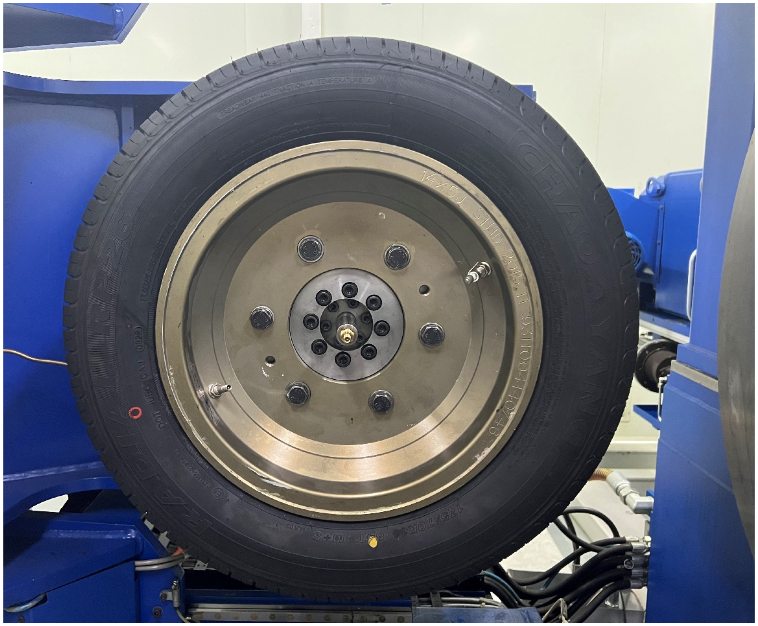
2.4. Experimental Verification

A sample of the FS-NPT was developed as shown in Figure 5. The spoke thickness was 6.6 mm. The spoke radius was 180°, and the spoke minimum width was 105 mm. Three-dimensional stiffness tests were carried out as experimental verification in CATARC (Tianjin) Automotive Engineering Research Institute Co., Ltd. (Tianjin, China), which is a standard-certified institution. The test rig used to test the non-pneumatic tires (FS-NPT) was the Tire Stiffness Test Machine (GDJ-4) made by Tianjin JIURONG Wheel Technology Co., Ltd. (Tianjin, China).

The test experiment used the static loading method. A vertical downward load was imposed on the center of the hub. The wheel deformation was recorded during the continuous loading process. Then the relationship between vertical load and vertical movement of the hub was obtained. Figure 6 shows the course of the center lines of the vertical stiffness for a normal load of 2800 N, which were obtained during the FEA model and experimental research. Figure 7 and Figure 8 show both simulation and test results of the lateral stiffness and longitudinal stiffness under a normal load of 2800 N, respectively. There may be four reasons for the differences between the obtained characteristics: using material data from the literature for the tread rubber and steel belt, disregarding the Mullins effect in the material model, neglecting the defects in the manufacturing process, and omitting the tread’s grooves.

Furthermore, we calculated the lateral and longitudinal stiffness, referring to the relevant national standards (GB/T 23663-2020). The calculation method for the vertical stiffness is shown in Equation (1). The lateral and longitudinal stiffness were calculated according to Equations (2) and (3), respectively.

$$K_{vertical}=\frac{F}{\delta }$$

(1)

where, $F$ is the normal load, which is 2800 N in this paper, and $\delta$ is the vertical movement of the center of the hub in the normal load.

$$K_{laterial}=\frac{F_1-F_2}{U_1-U_2}$$

(2)

where, $F_1$ is the normal load times 0.3 and plus 250 N, $F_2$ is the normal load times 0.3 and minus 250 N, $U_1$ is the lateral movement of the center of the hub with respect to the ground under the $F_1$ lateral force, $U_2$ is the lateral movement of the center of the hub with respect to the ground under the $F_2$ lateral force.

$$K_{longitudinal}=\frac{F_1-F_2}{U_1-U_2}$$

(3)

where, $F_1$ is the normal load times 0.3 and plus 250 N, $F_2$ is the normal load times 0.3 and minus 250 N, $U_1$ is the longitudinal movement of the center of the hub with respect to the ground under the $F_1$ longitudinal force, $U_2$ is the longitudinal movement of the center of the hub with respect to the ground under the $F_2$ longitudinal force.

According to the above three equations, the test and simulation results were calculated as shown in

Table 3. The stiffness of the FS-NPT sample.

Stiffness (N/mm)	Vertical Stiffness	Lateral Stiffness	Longitudinal Stiffness
Test	146.45	367.92	338.52
Simulation	149.75	400.00	333.33
Error	2.25%	8.72%	1.53%

.

The simulation results were verified by the experimental results. The error rate between the simulation results and test results was less than 10%. In particular, the error rate was less than 3% for the vertical stiffness and longitudinal stiffness. Accordingly, the finite element model was effective, and the results of the finite element analysis were reliable.

3. Parametric Studies of Geometry

3.1. Effects of Spoke Thickness on Three-Dimensional Stiffnesses of FS-NPT

First, the spoke thickness varied with a fixed spoke radius of 170° and a spoke width of 115 mm. Figure 9 shows the variation of three-dimensional stiffnesses, with respect to the change in the spoke thickness. We observed that, as the spoke thickness increased from 6.4 to 10 mm, the vertical stiffness of the FS-NPT increased almost linearly by 273.27%. The longitudinal stiffness of the FS-NPT also increased by 91.08%. However, the lateral stiffness of the FS-NPT decreased slightly, by only 3.82%, nearly maintaining the same value.

This implied that increasing the spoke material volume in the thickness direction made the FS-NPT stiffer and thereby increased the vertical stiffness. In addition, the load-carrying capacity of the FS-NPT increased. The bending of the spoke in the FS-NPT created a stiffer structure in the lateral direction. As the spoke thickness increased, the vertical deflection decreased and so did the spoke. Thus, spoke thickness had almost no influence on lateral stiffness.

3.2. Effects of Spoke Radius on Three-Dimensional Stiffnesses of FS-NPT

Second, the spoke radius varied with a fixed spoke thickness of 7.6 mm and a spoke width of 115 mm. When the spoke radius was less than 150° or more than 189°, the cross-section of the spokes in the sagittal plane were not a Fibonacci spiral. Thus, the spoke radius range for these parametric studies were bounded by these limits.

Figure 10 shows the variation of three-dimensional stiffnesses, with respect to the change in the spoke radius. We observed that, as the spoke radius increased from 150° to 189°, the vertical stiffness of the FS-NPT increased by 43.25%, and the longitudinal stiffness of the FS-NPT increased by 10.12%. The lateral stiffness of the FS-NPT was less affected, increasing by only 5.33%.

In the longitudinal and vertical direction, the spoke had a trend of buckling. The bigger the radius, the less the initial buckling trend. Hence, the increase in spoke radius had a positive effect on both longitudinal stiffness and vertical stiffness, and the load-carrying capacity of the FS-NPT increased.

3.3. Effects of Spoke Width on Three-Dimensional Stiffnesses of FS-NPT

Third, the spoke width varied with a fixed spoke thickness of 7.6 mm and a spoke radius of 170°. Figure 11 shows the variation of three-dimensional stiffnesses, with respect to the change in the spoke width. We observed that, as the spoke width increased from 100 to 145 mm, the vertical stiffness of the FS-NPT increased by 46.99% and the lateral stiffness of the FS-NPT increased by 8.41%. The longitudinal stiffness of the FS-NPT increased by 25.53%.

This implied that increasing the spoke material volume in the width direction made the FS-NPT stiffer and thereby increased the vertical stiffness and longitudinal stiffness. The increase in width also had a positive effect on lateral stiffness.

In general, the vertical stiffness exhibited the most sensitive response, and the longitudinal stiffness took second place. Comparatively, the lateral stiffness was only slightly responsive to the spoke width.

The results indicated that all three design variables of the spoke had a significant effect on the vertical and longitudinal stiffness, with the thickness having the greatest effect. The vertical stiffness was more sensitive to the spoke thickness than the longitudinal stiffness. We also found that the lateral stiffness remained nearly independent and was not coupled with the other two stiffnesses. Hence, the three-dimensional stiffness of the FS-NPT had a certain independent design space. This work demonstrated the advantages of non-pneumatic tires, especially FS-NPTs, in three-dimensional stiffness decoupling.

4. Optimization with Design of Experiments and Sensitivity Analysis

4.1. Optimization Problem Statement

In this section, geometric parameters are sought to attain the stiffness goals.

This FS-NPT was designed for the Chery eQ1 vehicle. The original pneumatic tire of this car was 175/70 R14 as shown in Figure 12. In this paper, we adjusted the profile and redesigned it. The outer diameter and the max section width of the FS-NPT were, respectively, 600 and 175 mm.

For the sake of the tire-damping performance, the vertical stiffness of the FS-NPT was the same as the original pneumatic tire, which was 218 N/mm, as shown in Figure 13. To ensure the braking and driving performance of the tires, the longitudinal stiffness should not be less than that of this car’s original pneumatic tire, which was 296 N/mm, as shown in Figure 14. Meanwhile, the longitudinal stiffness was a significant advantage of the FS-NPT, as mentioned above. Increasing the longitudinal stiffness of tires is not disadvantageous. Therefore, we defined the longitudinal stiffness target as 1.5 times 296 N/mm. Hence, the second target was longitudinal stiffness equal to 444 N/mm. It should be noted that the values can vary depending on a tire’s design requirement, resulting in different optimized values. Therefore, in this paper, we demonstrated an example of optimization for a set of values.

The objectives and constraints of the optimization are summarized as follows:

Objective Function:

Minimize the difference between the stiffness goals and the surrogate model of three-dimensional stiffness.

$$\underset{x_1,x_2,x_3}{\min }SSD$$

$$\mathrm{SSD}={\left(f_1\left(x_1,x_2,x_3\right)-g_1\right)}^2+w_2{\left(f_2\left(x_1,x_2,x_3\right)-g_2\right)}^2$$

where, SSD is the sum of squared differences (SSDs); $w_1$ is the weight of the first term in this equation; $f_1\left(x_1,x_2,x_3\right)$ is the approximate analytical RSM function of vertical stiffness. $g_1$ is the vertical stiffness goal. $w_2$ is the weight of the second term in this equation; $f_2\left(x_1,x_2,x_3\right)$ is the approximate analytical RSM function of longitudinal stiffness. $g_2$ is the longitudinal stiffness goal. For tires, longitudinal stiffness and vertical stiffness are equally important. Hence, we defined $w_1$ and $w_2$ with the same weights.

Subjected to Constraints:

The weight of the whole FS-NPT < 15 kg, which was equal to the weight of the run-flat tire with a similar specification. In the calculation of mass, the sea–land ratio of the tire tread pattern was defined as 0.4.

Design variables with limits:

6.4 mm < spoke thickness < 10 mm

150° < spoke radius < 189°

100 mm < spoke width < 145 mm

4.2. Design of Experiments and Design Sensitivity Study

To solve the optimization problem, first, a design of experiments (DOE) was conducted by running several numerical experiments on the design space defined by the limiting values of the design variables. Then data from the DOE was used to create a response surface model (RSM), which generated an approximate analytical function related to the design variables and the output response parameters. The analytical functions were optimized by solving the given optimization problem using different optimization algorithms.

In this study, a Latin hypercube DOE was conducted to investigate the responses of vertical stiffness, longitudinal stiffness, and weight in combination with the spoke design variables. The Latin hypercube is a multi-dimensional extension of the Latin squares sampling method [15]. Using the Latin hypercube sampling methods, a total of 50 designs were generated, as shown in

Table 4. Design of experiments using Latin hypercube sampling.

No	Thickness (mm)	Radius (°)	Width (mm)	Vertical Stiffness (N/mm)	Longitudinal Stiffness (N/mm)	Weight (kg)
1	9.34	153.98	125.71	549.53	724.10	17.67
2	9.05	175.47	130.31	589.68	717.05	17.13
3	7.94	174.67	127.55	413.18	644.16	16.26
4	7.28	186.61	126.63	374.13	601.33	15.57
5	8.60	177.86	117.45	489.42	725.02	16.35
6	8.90	176.27	104.59	477.29	649.71	16.13
7	8.53	162.73	123.88	456.85	694.45	16.80
8	8.75	165.92	138.57	534.93	734.53	17.38
9	8.02	157.96	145.00	420.62	690.83	17.16
10	7.36	150.00	110.10	235.97	513.61	15.75
11	7.14	172.29	103.67	231.04	472.56	15.05
12	7.06	182.63	140.41	345.47	598.87	15.82
13	8.31	189.00	122.96	522.89	691.40	16.13
14	9.56	165.12	129.39	609.95	745.13	17.70
15	8.68	188.20	109.18	522.24	673.71	15.95
16	8.97	178.65	144.08	619.86	713.83	17.45
17	6.40	179.45	128.47	215.18	446.84	15.10
18	9.41	155.57	139.49	598.77	723.84	18.19
19	6.84	185.82	106.43	242.90	465.59	14.76
20	9.27	161.14	101.84	465.71	678.22	16.54
21	8.09	184.22	136.73	496.81	687.78	16.46
22	8.16	167.51	100.00	338.66	587.28	15.65
23	7.87	181.84	102.76	352.48	600.10	15.34
24	7.43	151.59	132.14	298.89	589.85	16.44
25	7.80	173.08	141.33	419.32	658.35	16.57
26	9.93	170.69	105.51	594.52	701.78	16.93
27	7.72	168.31	113.78	326.73	584.79	15.80
28	9.63	173.88	118.37	620.46	705.32	17.16
29	6.91	156.37	143.16	267.94	552.42	16.23
30	7.58	181.04	115.61	350.61	599.80	15.55
31	6.77	170.69	137.65	253.65	525.59	15.72
32	7.65	163.53	133.06	363.25	632.23	16.40
33	8.24	157.16	107.35	357.35	623.34	16.14
34	10.00	180.24	135.82	740.63	708.95	17.92
35	9.12	187.41	134.90	656.96	718.51	17.09
36	9.78	169.10	142.24	694.54	768.17	18.24
37	9.85	161.94	116.53	590.47	715.02	17.51
38	6.62	160.35	131.22	206.38	487.11	15.62
39	6.47	154.78	119.29	159.84	374.98	15.29
40	9.49	185.02	122.04	651.35	691.80	16.97
41	7.50	158.76	121.12	307.92	583.29	16.03
42	8.31	150.80	120.20	389.01	650.34	16.76
43	7.21	159.55	100.92	210.99	466.40	15.20
44	9.71	183.43	108.27	615.93	670.59	16.65
45	9.19	152.39	111.02	481.31	680.89	17.04
46	6.55	177.06	114.69	197.43	427.28	14.90
47	6.69	164.33	111.94	184.18	413.80	15.11
48	8.46	153.18	133.98	452.12	688.84	17.29
49	8.82	166.71	112.86	472.98	679.73	16.55
50	6.99	169.90	123.88	257.51	515.68	15.55

. Each design represented a different combination of design variables. A DOE was performed for two cases: upper and lower bounds of the design variables.

Because of the need for a large number of geometric models and finite element models in the optimization process, we conducted the out secondary development of ABAQUS based on Python. We achieved the automatic production of the geometries of all the DOE designs, automatic establishment and automatic submission of the finite element models in ABAQUS, and automatic post-processing of simulation data. The detailed code of the automatic post-processing of simulation data can be found in Appendix A.

The effect of the design variables on the response parameter was studied using the Pareto chart of the standardized effects, as shown in Figure 15 [16]. This determined the absolute value of the effects, as indicated by the red line on the chart. The effect of any parameter that extends past the line is potentially important. The line indicating the absolute value corresponds to alpha = 0.05, and the effects were calculated at 95% confidence levels. Figure 15a shows that all the design variables play an important role in affecting the vertical stiffness of the NPT. However, the spoke thickness was the most important variable. We also observed that a combined effect of the spoke thickness and spoke width (AC in Figure 15a) also played a considerable role in the affecting weight. Spoke thickness and spoke radius also had the same effect (AB in Figure 15a).

Figure 15b shows the Pareto chart of the longitudinal stiffness response of the NPT. The influence of the design variables on the longitudinal stiffness was not similar to their influence on the vertical stiffness response. Figure 15b indicates that the spoke thickness and width played an important role in affecting the longitudinal stiffness of the NPT. Figure 15b shows that the spoke radius (shown as B) had no potential effect on the longitudinal stiffness of the NPT. Hence, the radius of the spokes was a decoupling parameter.

Figure 15c shows the Pareto chart for the weight. The spoke thickness, the spoke radius, the spoke width, and their interaction effect were important factors affecting weight. However, their interaction effect had significantly less influence, as shown in Figure 15c.

4.3. Response Surface Model (RSM)

The RSM is an approximation technique used to explore the nonlinear functional relationship between the design variables and the output parameters [17]. The quadratic RSM is the most common model in research. A second-order polynomial form is:

$$\mathrm{Vertical} \mathrm{stiffness}: f_v(x_1,x_2,x_3)=350.669+67.988x_1-16.384x_2+3.477x_3\pm 2.066x_1^2+0.046x_2^2-0.022x_3^2+0.309x_1{x}_2+0.397x_1{x}_3+0.008x_2{x}_3$$

$$\mathrm{Longitudinal} \mathrm{stiffness}: f_l(x_1,x_2,x_3)=-5406+815.491{𝑥}_1-14.041{𝑥}_2+16.513{𝑥}_3-31.357x_1^2-0.014x_2^2-0.024x_3^2-0.808{𝑥}_1{𝑥}_2-0.670{𝑥}_2{𝑥}_3-0.017{𝑥}_2{𝑥}_3$$

$$\mathrm{Weight}: f_w(x_1,x_2,x_3)=9.629+0.719x_1-0.021x_2+0.037x_3-0.008x_1^2-7.984x_3^2- 0.002x_1{x}_2+0.004x_1{x}_3$$

Input Parameters: x₁ = spoke thickness; x₂ = spoke radius; x₃ = spoke width.

Response Parameters: $f_v$($x_1,x_2,x_3$) = vertical stiffness; $f_l$($x_1,x_2,x_3$) = longitudinal stiffness; $f_w$($x_1,x_2,x_3$) = weight.

The $R^2$ values of the coefficient determination of the quadratic RSM for the vertical stiffness, longitudinal stiffness and weight were 0.999, 0.985, and 0.999, respectively. All three coefficient determinations were between 0.9 and 1, which means the RSM was an extremely high correlation. The RSM approximation can be used to explore the nonlinear functional relationship between the design variables and the output parameters.

An RSM for the vertical stiffness of the NPT as functions of the thickness and the width of the spokes is shown in Figure 16. Figure 17 shows the longitudinal stiffness of the NPT as functions of the thickness and the width of the spokes. Figure 18 shows the weight of the NPT as the functions of the thickness and the width of the spokes.

4.4. Optimization Algorithms

The response surface model in this paper is a nonlinear constrained and continuous optimization problem. Three optimization algorithms were selected based on the nature of the problem. They are adaptive simulated annealing (ASA) [18], multi-objective particle swarm optimization (MOPSO) [19], and sequential quadratic programming (NLPQL) [20]. The reason for selecting these three optimization algorithms was to ensure that the global optimum was achieved using all three algorithms.

The optimization results achieved using the three algorithms are shown in

Table 5. Optimization results achieved using three algorithms.

Optimization/ Validation	Spoke Thickness (mm)	Spoke Radius (°)	Spoke Width (mm)	Vertical Stiffness (N/mm)	Longitudinal Stiffness (N/mm)	Weight (kg)
ASA	6.87	182.09	101.30	218.00	444.00	14.69
MOPSO	6.91	177.24	104.05	216.86	453.89	14.85
NLPQL	7.00	171.97	100	201.22	443.88	14.85

. The results include the optimal values of the design variables and their corresponding output response using the adaptive simulated annealing (ASA), multi-objective particle swarm optimization (MOPSO), and sequential quadratic programming (NLPQL). The optimization result obtained by ASA was the most consistent with the optimization objective and had the least mass. Hence, the results achieved through ASA optimization were validated using the FEA model with ABAQUS by setting the design variables to the optimum values and performing the finite element analysis. The results are also shown in

Table 6. Optimization results and FEA validation.

Optimization/ Validation	Spoke Thickness (mm)	Spoke Radius (°)	Spoke Width (mm)	Vertical Stiffness (N/mm)	Longitudinal Stiffness (N/mm)	Weight (kg)
ASA	6.87	182.09	101.30	218.00	444.00	14.69
FEA	6.87	182.09	101.30	216.30	444.92	14.67
Error %				0.79%	0.21%	0.14%

. We observed that the optimization results matched the results from FEA with an error percentage of less than 1% for all three response parameters. It should be noted that the results of the optimization achieved are specific to this problem. Different results can be achieved with different bounds for the constraints, such as different weights.

It was important to study the characteristics of the NPT with the optimized configuration. These characteristics were compared to the previously used configuration (non-optimized) of the NPT. They were plotted together to show the improvement in design from the optimization, as shown in Figure 19 and Figure 20. The optimum values obtained using the ASA algorithm and the reference values of the design variables (the previously used NPT configuration) used for comparison are shown in

Table 7. Values of the design and response variables (reference and optimized configuration).

Configuration	Spoke Thickness (mm)	Spoke Radius (°)	Spoke Width (mm)	Vertical Stiffness (N/mm)	Longitudinal Stiffness (N/mm)	Weight (kg)
Reference	6.6	180	105	149.75	338.52	14.65
Optimized	6.87	182.09	101.30	216.30	444.92	14.67

. Table 7 indicates that the optimization resulted in a considerable increase in the spoke thickness, a slight increase in the spoke radius, and a decrease in the spoke width. The optimization algorithm kept the constraint on weight nears its higher limit.

The variation in the design parameters increased both the longitudinal stiffness and vertical stiffness of the FS-NPT, but with considerably different degrees of design sensitivity. It was obvious that the spoke thickness significantly affected all the response variables. Hence, for the FS-NPT, increasing the target for the vertical stiffness will inevitably lead to an increase in weight when the other parameters are fixed. Vertical stiffness and longitudinal stiffness are coupled to a certain extent, but the predetermined goal can be achieved by different design variables affecting them to different degrees.

5. Conclusions and Future Work

Parametric, sensitivity, and optimization studies were conducted to investigate the effects of the spoke thickness, the spoke radius, and the spoke width on vertical stiffness, lateral stiffness, and longitudinal stiffness of the FS-NPT. In the meantime, the weight of the NPT was also taken as a constraint. The major findings of these studies are as follows:

• The parametric study showed that variation in all three design parameters had no considerable effect on the lateral stiffness. The lateral stiffness kept nearly independent and was not coupled with the other two stiffnesses.
• The sensitivity analysis with the DOE and Pareto charts demonstrated that the spoke thickness was the most important design parameter regarding vertical stiffness, longitudinal stiffness, and weight. The spoke radius had no potential effect on the longitudinal stiffness of the NPT.
• Optimized geometric parameters were found: a spoke thickness of 6.87 mm, a spoke radius of 182.09°, and a spoke width of 101.30 mm under a constraint on weight. The optimization result was completely consistent with the stiffness target, and the error rate was less than 1%.
• Vertical stiffness and longitudinal stiffness were coupled to a certain extent, but the predetermined goals were achieved by different design variables affecting them to different degrees. The optimization results indicated that the FS-NPT has a large stiffness design range. The different stiffness targets were achieved by adjusting different combinations of design variables, and the tire mass did not increase significantly.

NPTs can be modeled with various geometric and material selections. This study demonstrated a design solution for an NPT related to the different stiffness targets. In future work, while maintaining all three stiffness parameters of the FS-NPT, the lightweight design of the FS-NPT will be the next research focus.

References

1. Yoo, S.; Uddin, M.S.; Heo, H.; Ju, J.; Kim, D.M.; Choi, S.J. Deformation and heat generation in a nonpneumatic tire with lattice spokes (No. 2015-01-1512). SAE Technical Paper, 14 April 2015; p. 9. [Google Scholar] [CrossRef]
2. Narasimhan, A.; Ziegert, J.; Thompson, L. Effects of material properties on static load-deflection and vibration of a non-pneumatic tire during high-speed rolling. SAE Int. J. Passeng. Cars-Mech. Syst. 2011, 4, 59–72. [Google Scholar] [CrossRef]
3. Rhyne, T.B.; Cron, S.M. Development of a non-pneumatic wheel. Tire Sci. Technol. 2006, 34, 150–169. [Google Scholar] [CrossRef]
4. Gibert, J.M.; Ananthasayanam, B.; Joseph, P.F.; Rhyne, T.B.; Cron, S.M. Deformation Index–Based Modeling of Transient, Thermo-mechanical Rolling Resistance for a Nonpneumatic Tire. Tire Sci. Technol. 2013, 41, 82–108. [Google Scholar] [CrossRef]
5. Zhao, Y.; Du, X.; Lin, F.; Wang, Q.; Fu, H. Static stiffness characteristics of a new non-pneumatic tire with different hinge structure and distribution. J. Mech. Sci. Technol. 2018, 32, 3057–3064. [Google Scholar] [CrossRef]
6. Gasmi, A.; Joseph, P.F.; Rhyne, T.B.; Cron, S.M. Development of a two-dimensional model of a compliant non-pneumatic tire. Int. J. Solids Struct. 2012, 49, 1723–1740. [Google Scholar] [CrossRef] [Green Version]
7. Narasimhan, A. A Computational Method for Analysis of Material Properties of a Non-Pneumatic Tire and Their Effects on Static Load-Deflection, Vibration, and Energy Loss from Impact Rolling over Obstacles. Master’s Thesis, Clemson University, Clemson, SC, USA, August 2010. Available online: https://tigerprints.clemson.edu/all_theses/1003 (accessed on 1 August 2022).
8. Dhrangdhariya, P.; Soumyadipta, M.; Beena, R. Effect of spoke design and material nonlinearity on non-pneumatic tire stiffness and durability performance. arXiv 2021, arXiv:2103.03637. [Google Scholar] [CrossRef]
9. Wu, T.; Li, M.; Zhu, X.; Lu, X. Research on non-pneumatic tire with gradient anti-tetrachiral structures. Mech. Adv. Mater. Struct. 2021, 28, 2351–2359. [Google Scholar] [CrossRef]
10. Rugsaj, R.; Suvanjumrat, C. Proper Radial Spokes of Non-Pneumatic Tire for Vertical Load Supporting by Finite Element Analysis. Int. J. Automot. Technol. 2019, 20, 801–812. [Google Scholar] [CrossRef]
11. Xu, T.; Zhang, B. The Invention Relates to a High Speed and High Load Non-Pneumatic Tire and a Preparation Method Thereof. Patent CN 111152600B, 2019. [Google Scholar]
12. Li, C.; Ji, A.; Cao, Z. Stressed Fibonacci spiral patterns of definite chirality. Appl. Phys. Lett. 2007, 90, 164102. [Google Scholar] [CrossRef]
13. Paul, B.G. Pattern formation in shoots: A likely role for minimal energy configurations of the tunica. Int. J. Plant Sci. 1992, 153, S59–S75. [Google Scholar]
14. Lee, W.S.; Su, T.T. Mechanical properties and microstructural features of aisi 4340 high-strength alloy steel under quenched and tempered conditions. J. Mater. Process. Technol. 1999, 87, 198–206. [Google Scholar] [CrossRef]
15. Fang, K.T.; Li, R.; Sudjianto, A. Design and Modeling for Computer Experiments; Chapman and Hall/CRC: New York, NY, USA, 2005. [Google Scholar]
16. Barrentine, L.B. An Introduction to Design of Experiments: A Simplified Approach; American Society for Quality: Milwaukee, WI, USA, 1999. [Google Scholar]
17. Myers, R.H.; Montgomery, D.C.; Anderson-Cook, C.M. Response Surface Methodology: Process and Product Optimization Using Designed Experiments; John Wiley & Sons: Hoboken, NJ, USA, 2016. [Google Scholar]
18. Granville, V.; Krivanek, M.; Rasson, J.-P. Simulated annealing: A proof of convergence. IEEE Trans. Pattern Anal. Mach. Intell. 1994, 16, 652–656. [Google Scholar] [CrossRef]
19. Coello, C.A.C.; Lechuga, M.S. MOPSO: A proposal for multiple objective particle swarm optimization. In Proceedings of the 2002 Congress on Evolutionary Computation. CEC’02 (Cat. No. 02TH8600), Honolulu, HI, USA, 12–17 May 2002; Volume 2, pp. 1051–1056. [Google Scholar]
20. Boggs, P.T.; Tolle, J.W. Sequential quadratic programming for large-scale nonlinear optimization. J. Comput. Appl. Math. 2000, 124, 123–137. [Google Scholar] [CrossRef]
Figure 1. The detailed description of the FS-NPT.
Machines 10 01183 g001
Figure 2. The radial design feature of the spoke in a 2D plane of the FS-NPT.
Machines 10 01183 g002
Figure 3. Comparison of the tensile nominal stress–nominal strain curves of the PU material.
Machines 10 01183 g003
Figure 4. The finite element model of the FS-NPT.
Machines 10 01183 g004
Figure 5. A sample of the FS-NPT.
Machines 10 01183 g005
Figure 6. The courses of the center lines of the vertical stiffness in the test and simulation.
Machines 10 01183 g006
Figure 7. The courses of the center lines of the lateral stiffness in the test and simulation.
Machines 10 01183 g007
Figure 8. The courses of the center lines of the longitudinal stiffness in the test and simulation.
Machines 10 01183 g008
Figure 9. Effects of the spoke thickness on the three-dimensional stiffnesses of the FS-NPT.
Machines 10 01183 g009
Figure 10. Effects of the spoke radius on the three-dimensional stiffnesses of the FS-NPT.
Machines 10 01183 g010
Figure 11. Effects of the spoke width on the three-dimensional stiffnesses of the FS-NPT.
Machines 10 01183 g011
Figure 12. The original pneumatic tire of the Chery eQ1 vehicle (175/70 R14).
Machines 10 01183 g012
Figure 13. The vertical force vs. vertical displacement of the original pneumatic tire (175/70 R14).
Machines 10 01183 g013
Figure 14. The longitudinal force vs. longitudinal displacement of the original pneumatic tire (175/70 R14).
Machines 10 01183 g014
Figure 15. Pareto chart for (a) vertical stiffness; (b) longitudinal stiffness; and (c) weight.
Machines 10 01183 g015
Figure 16. RSM for the vertical stiffness of the NPT as functions of the thickness and width of spokes.
Machines 10 01183 g016
Figure 17. RSM for the longitudinal stiffness of the NPT as functions of the thickness and width of spokes.
Machines 10 01183 g017
Figure 18. RSM for the weight of the NPT as functions of the thickness and width of spokes.
Machines 10 01183 g018
Figure 19. Vertical stiffness of the reference and optimized configurations.
Machines 10 01183 g019
Figure 20. Longitudinal stiffness of the reference and optimized configurations.
Machines 10 01183 g020