
Wind Turbine Blade Defect Detection Based on Acoustic Features and Small Sample Size

Abstract
:1. Introduction
2. Materials and Methods
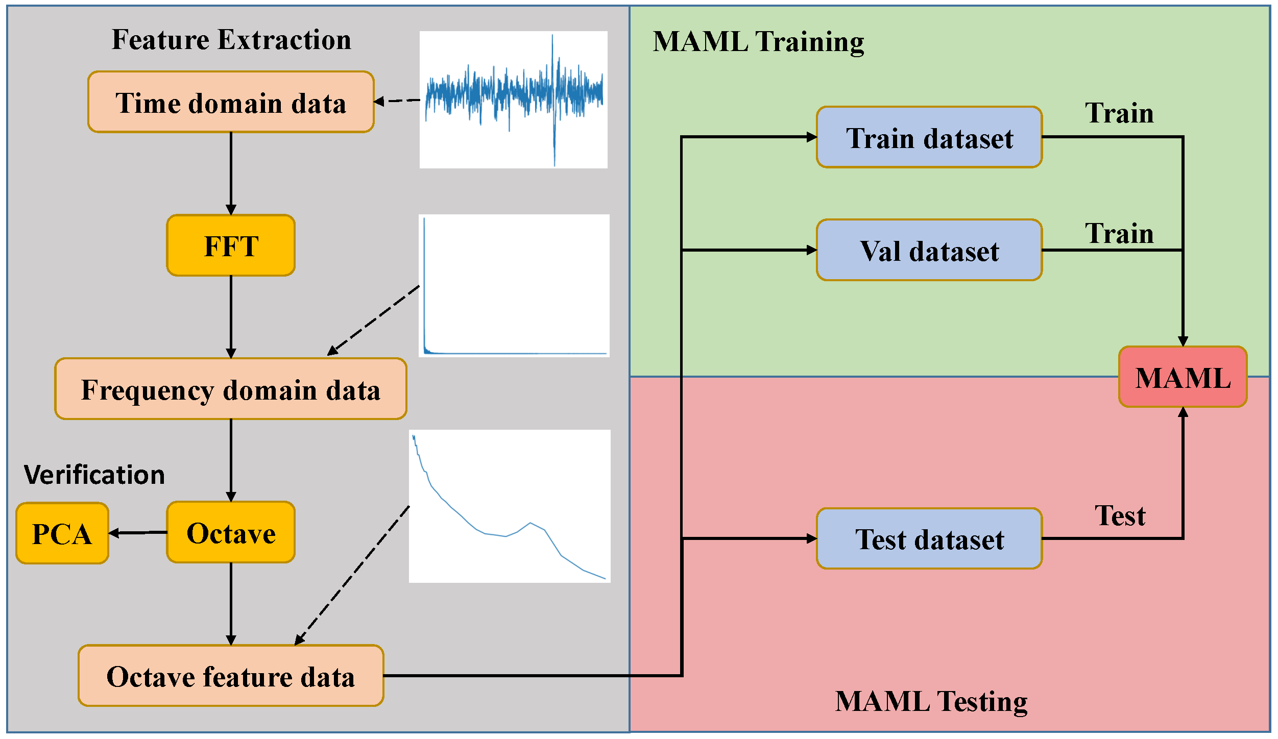
2.1. Study Workflow
- (1)
- We used fast Fourier transform (FFT) to convert the time-domain signal into the frequency domain;
- (2)
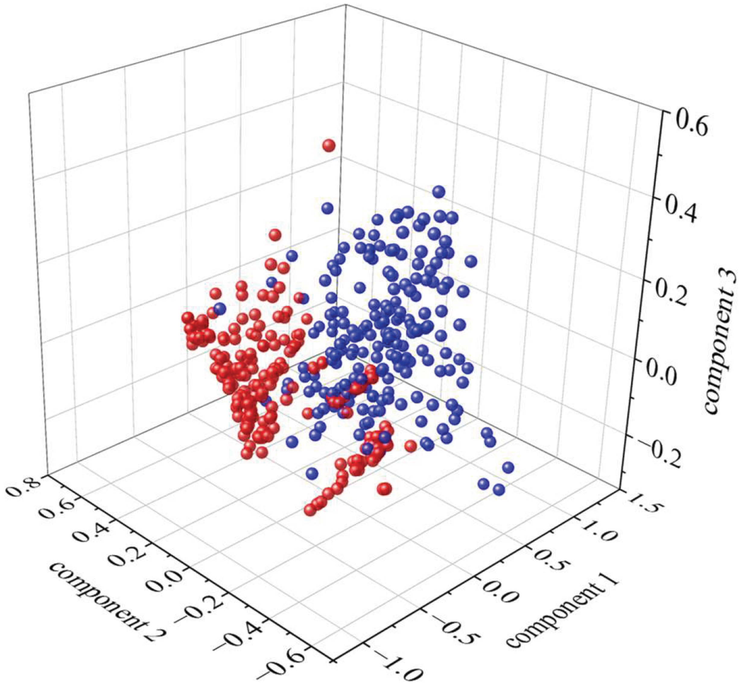
- We used the octave feature extraction algorithm to extract the features of the acoustic signals of wind turbine blades, then used principal component analysis (PCA) to analyze the spatial distribution of the samples;
- (3)
- We used the training set to train MAML-ANN, and used the validation set to adjust the training direction of the model;
- (4)
- We tested the performance of MAML-ANN using the test set, and compared its results with those of traditional ANN.
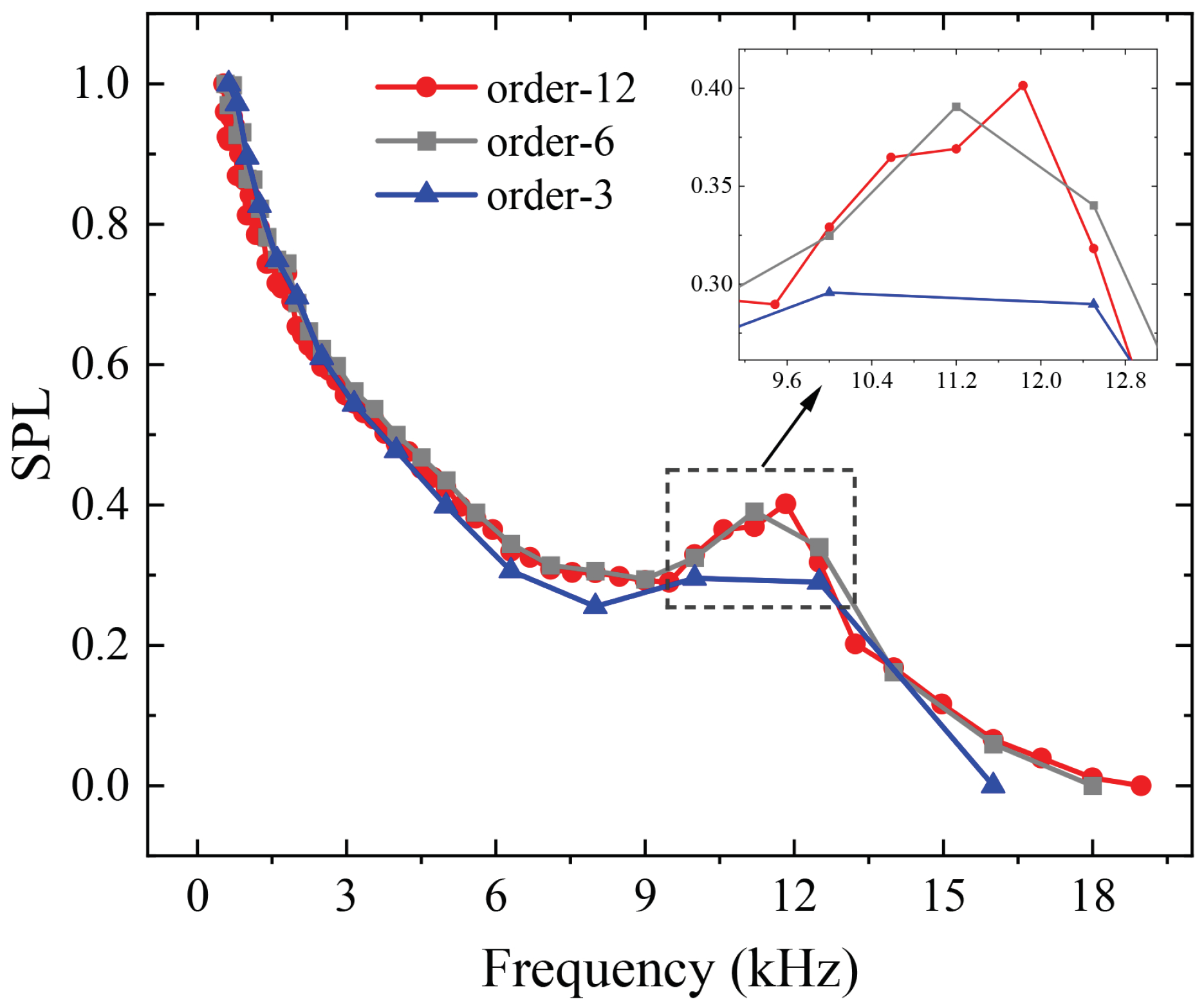
2.2. Octave Feature Extraction
- (1)
- Divide the frequency bands according to the octave center frequency. The two methods to determine the octave center frequency are constant increase and constant percentage increase. In our method, we adopted the “GB3240-82 Preferred frequencies for the acoustic measurement” standard, which divides the discrete frequency domain into frequency bands with a constant bandwidth ratio. The reference frequency was 1000 Hz. The center frequency, lower cut-off frequency, and upper cut-off frequency of the frequency band can be expressed as:where n represents an integer (0, ±1, ±2, ±3, ...); N is the order of the octave (1, 1/2, 1/3, 1/6, 1/12, 1/24, ...).
- (2)
- Calculate the sound pressure (SP) of each frequency band. The square sum of frequency points was used for each frequency band to obtain the SP, which can be expressed as:where is the SP of the frequency band, is the lower cut-off frequency, is the upper cut-off frequency, and is the amplitude of the frequency point.
- (3)
- Calculate the sound pressure level (SPL) of each SP. Due to the logarithmic relation between human ears and frequency, SP must be converted into SPL. SPL can be expressed as:where Pa, and denotes the SP values.
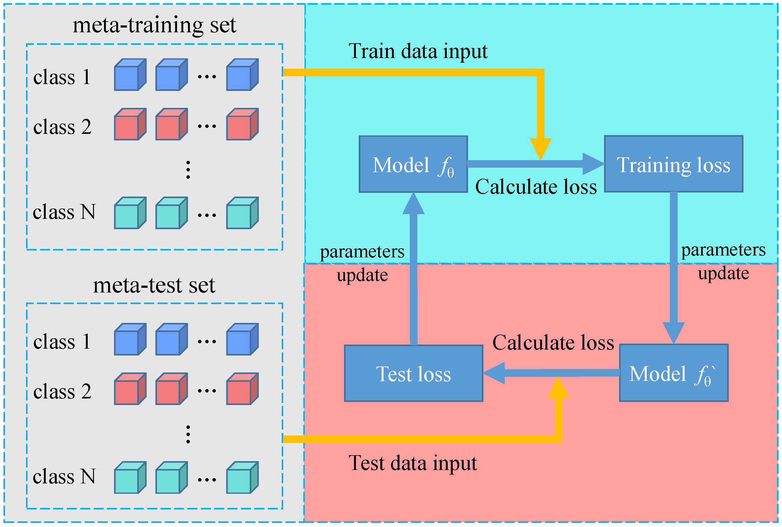
2.3. Model-Agnostic Meta-Learning
- (1)
- N-way K-shot
- (2)
- Secondary gradient descent
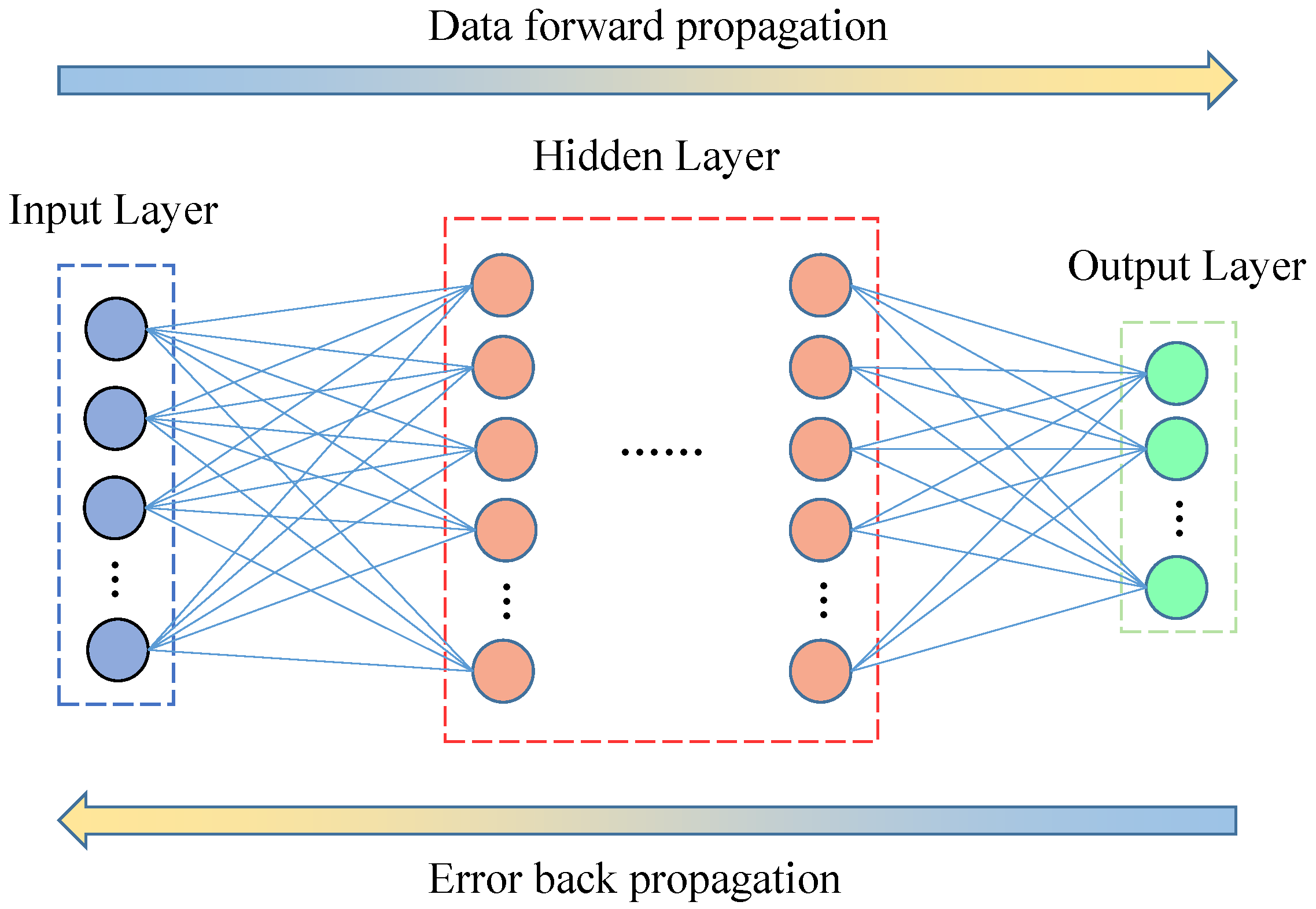
2.4. Artificial Neural Network
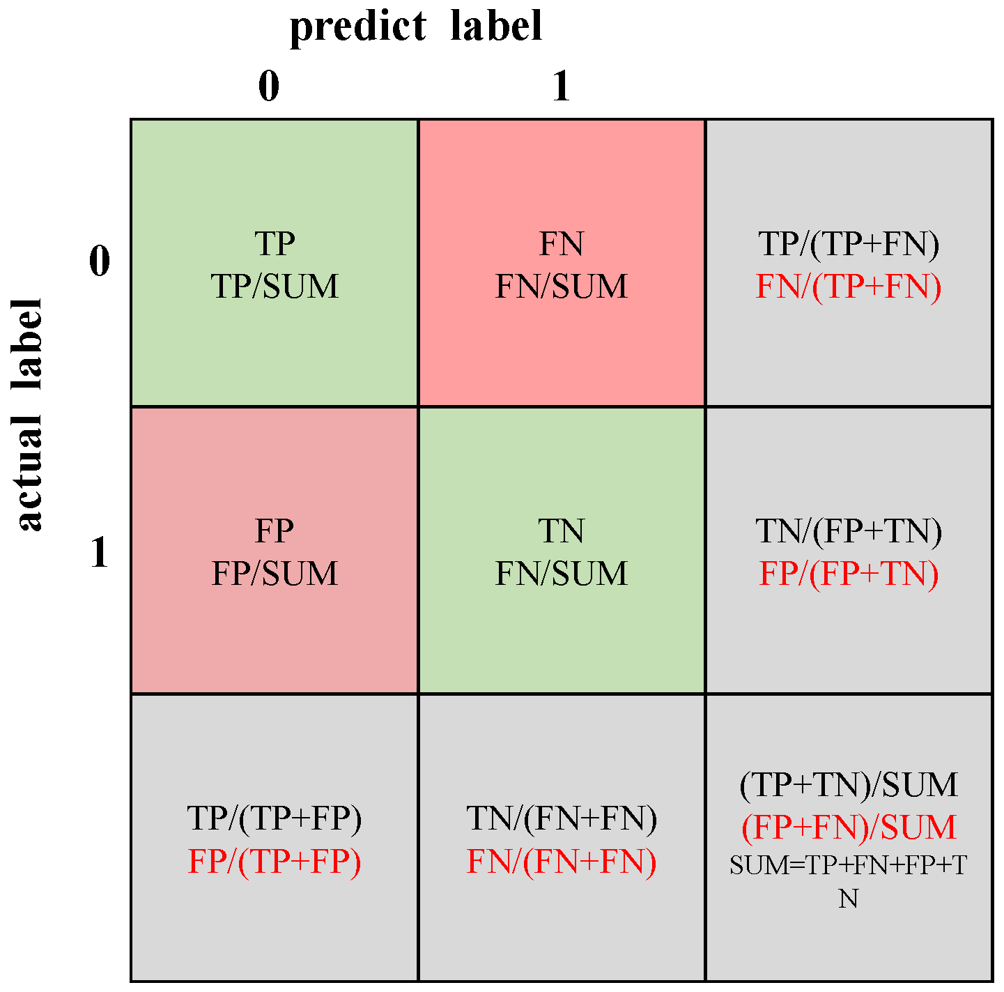
2.5. Evaluation Metrics
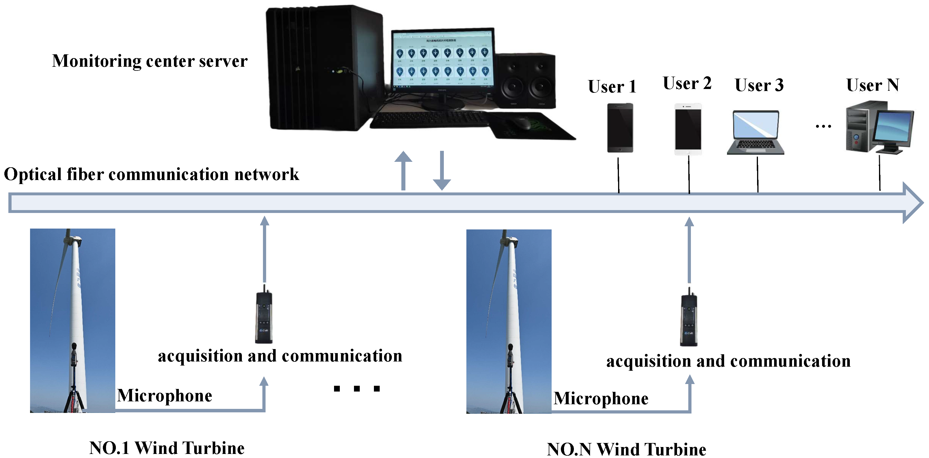
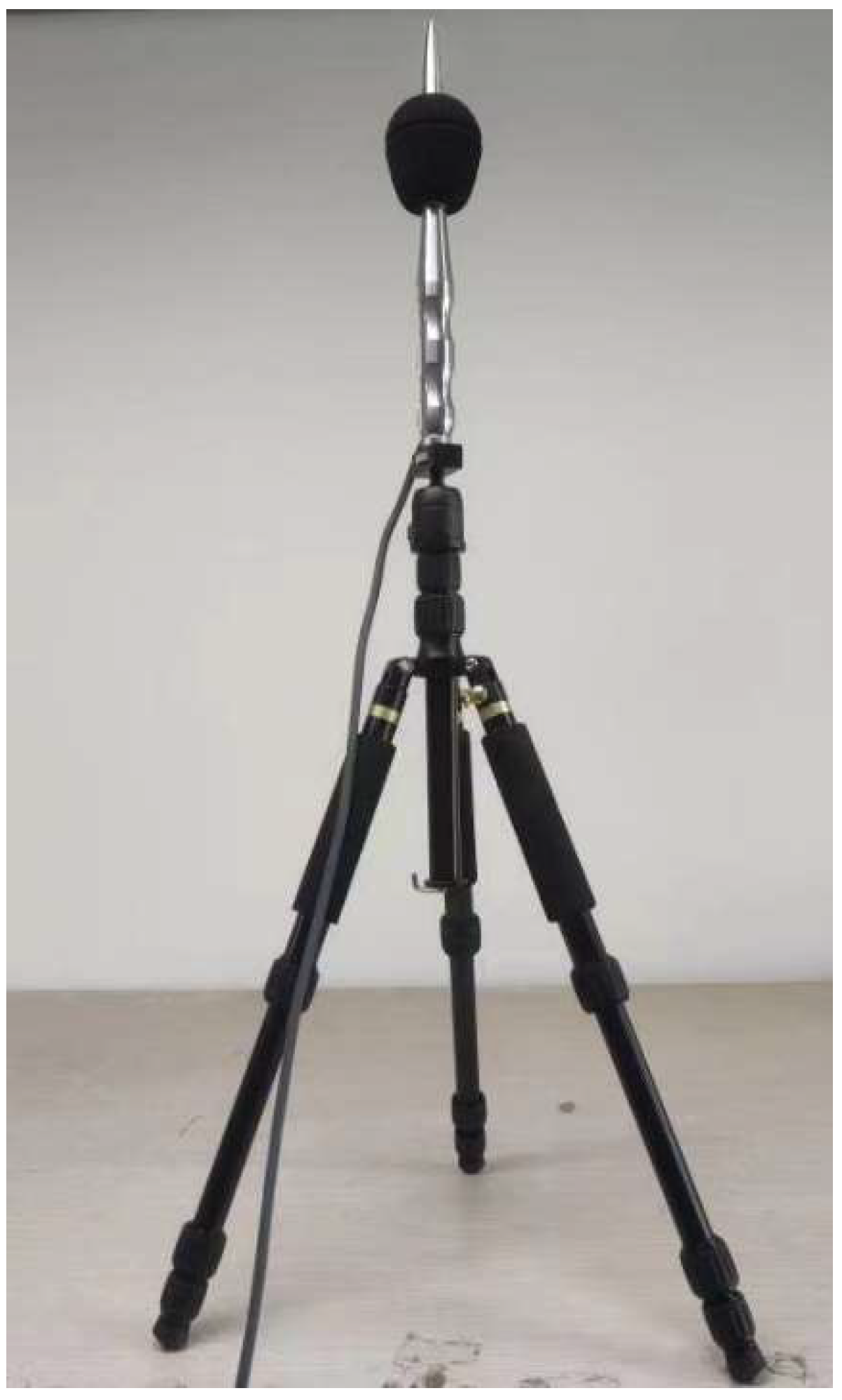
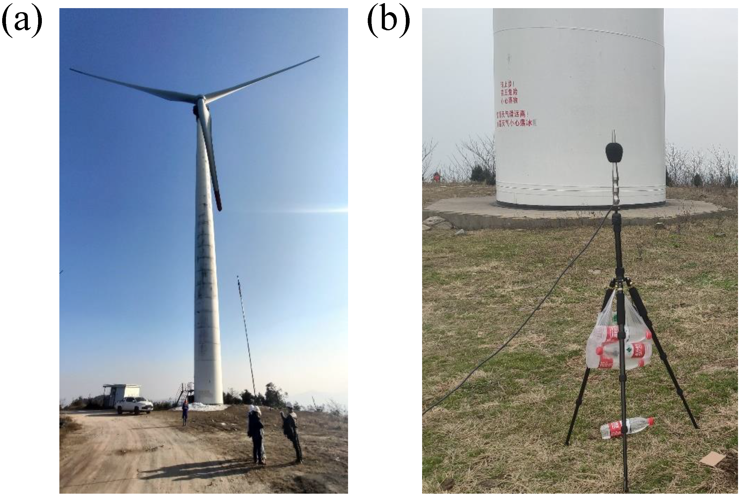
2.6. Front-End Acoustic Acquisition System
3. Results
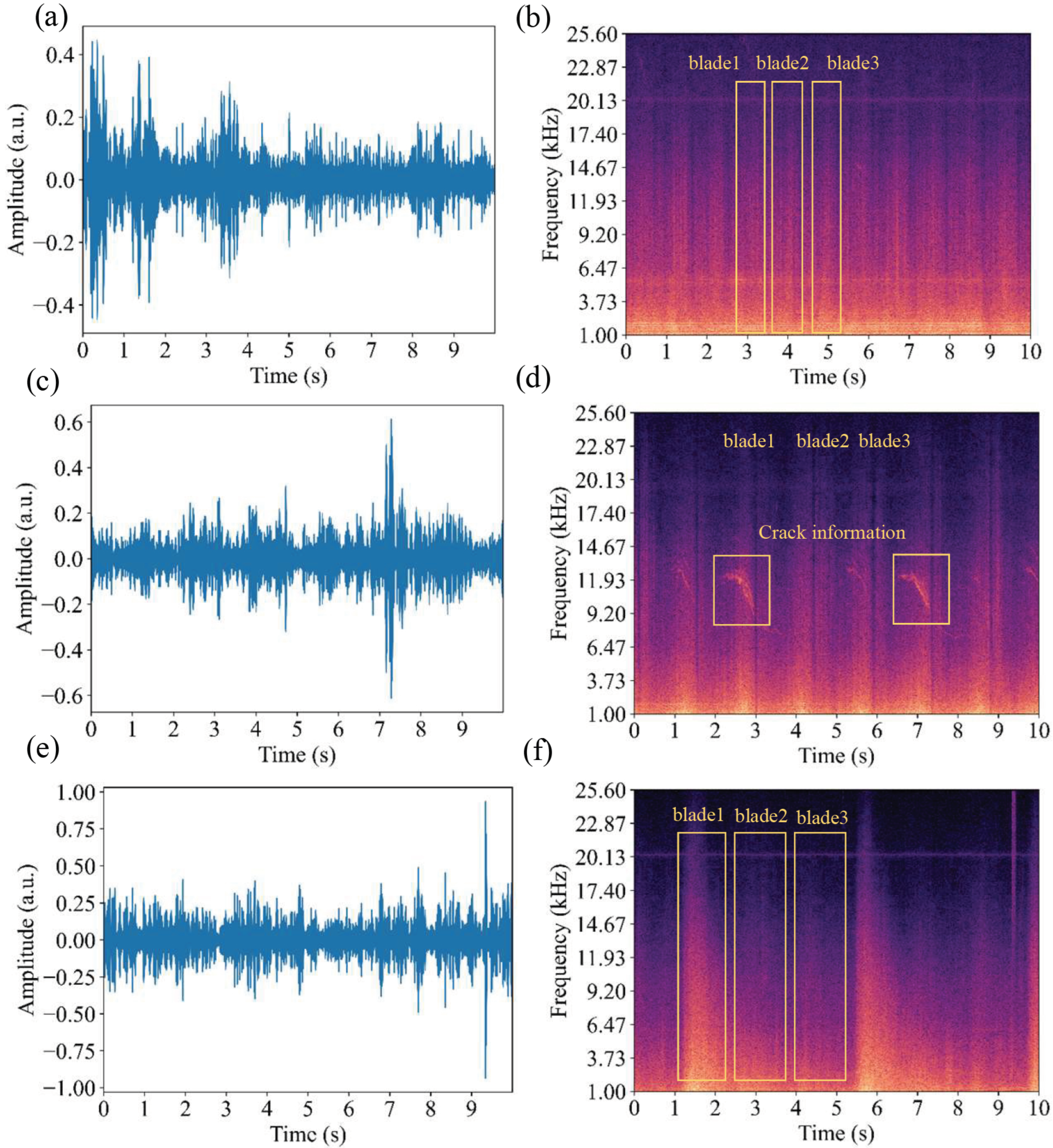
3.1. Data Acquisition
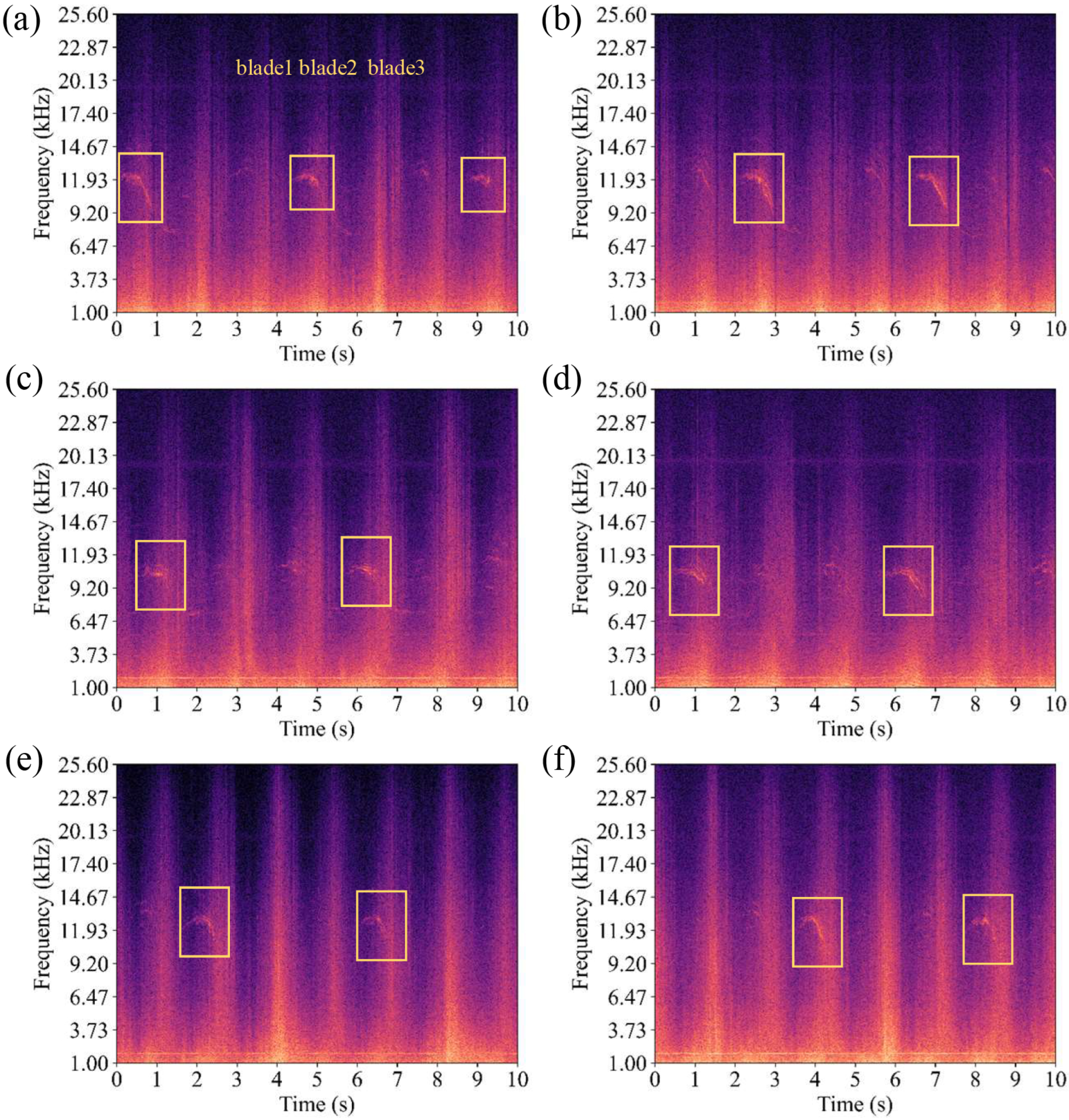
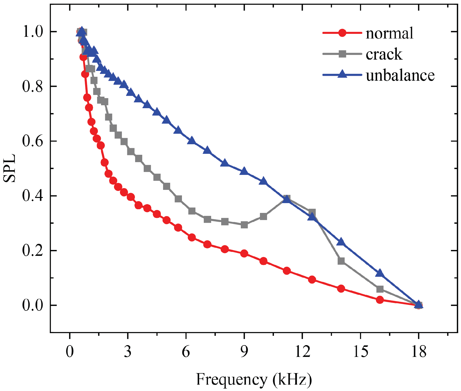
3.2. Acoustic Feature Extraction
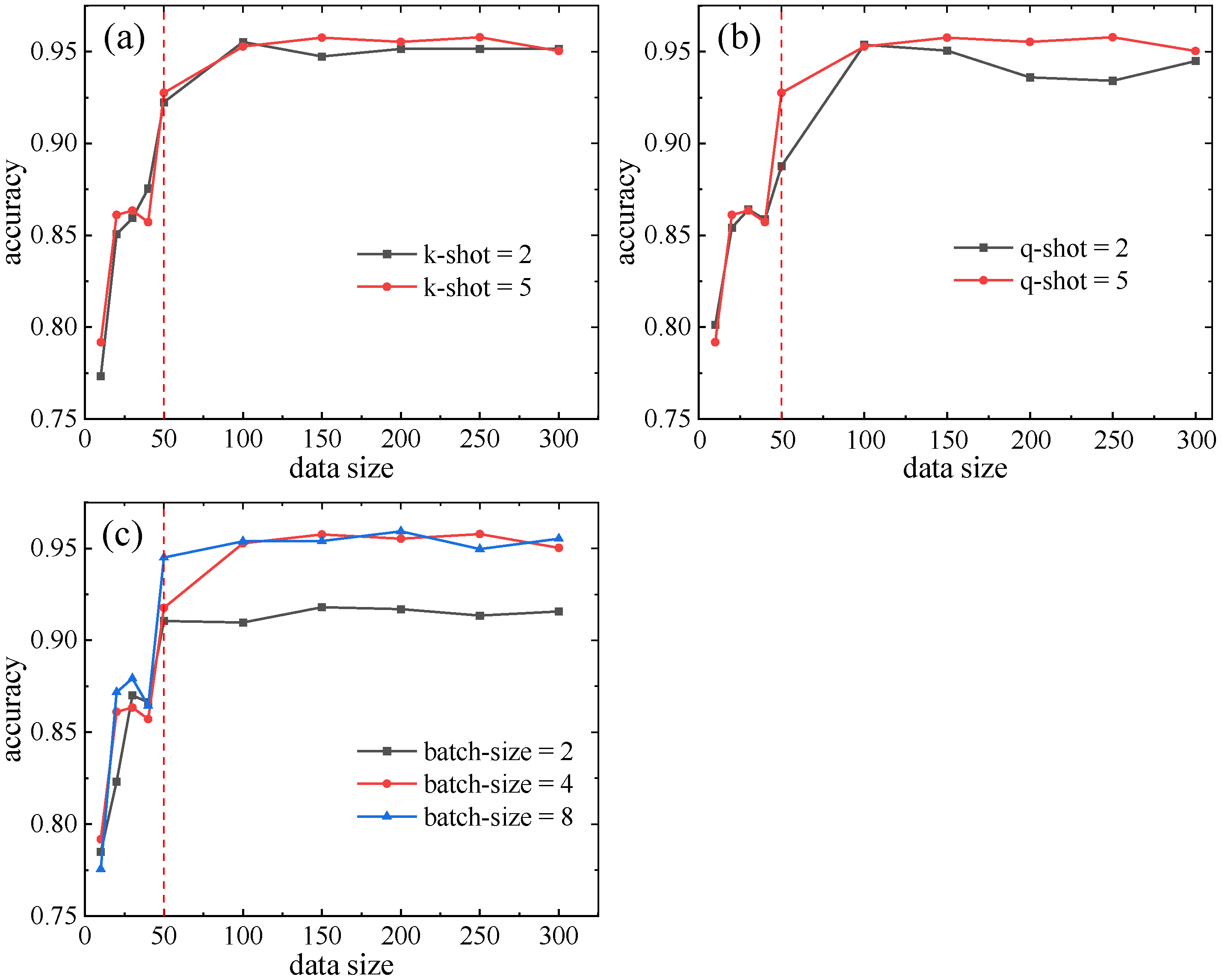
3.3. Hyperparameter Selection
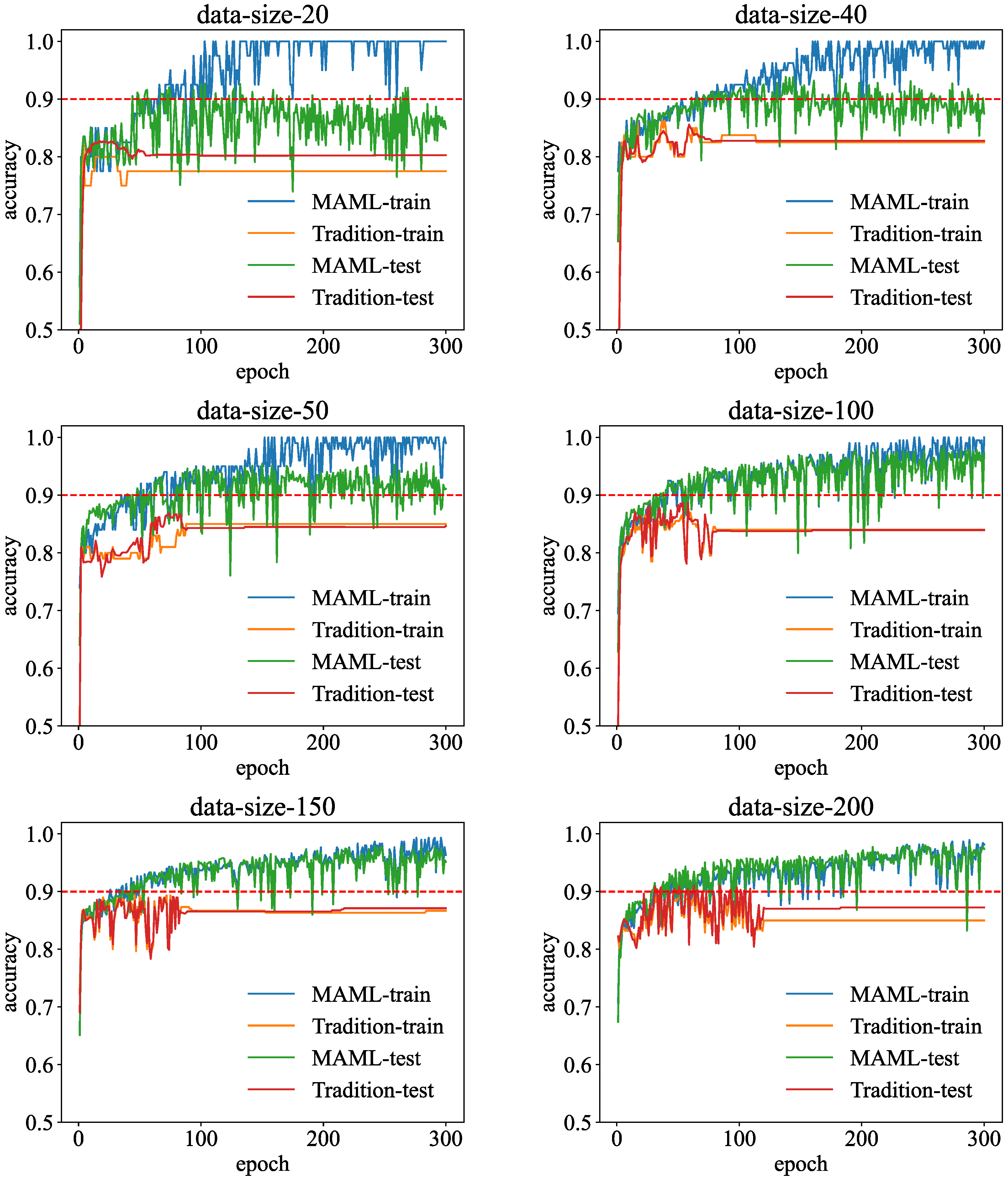
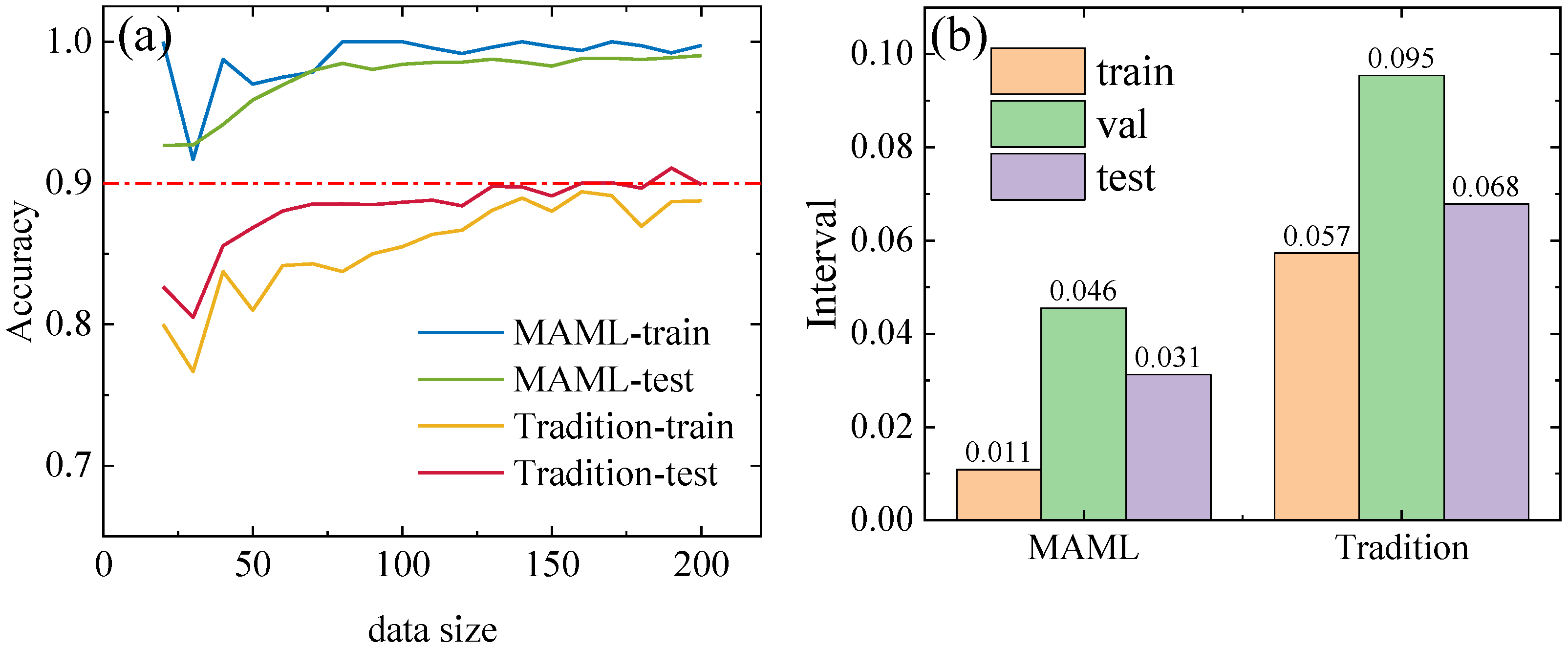
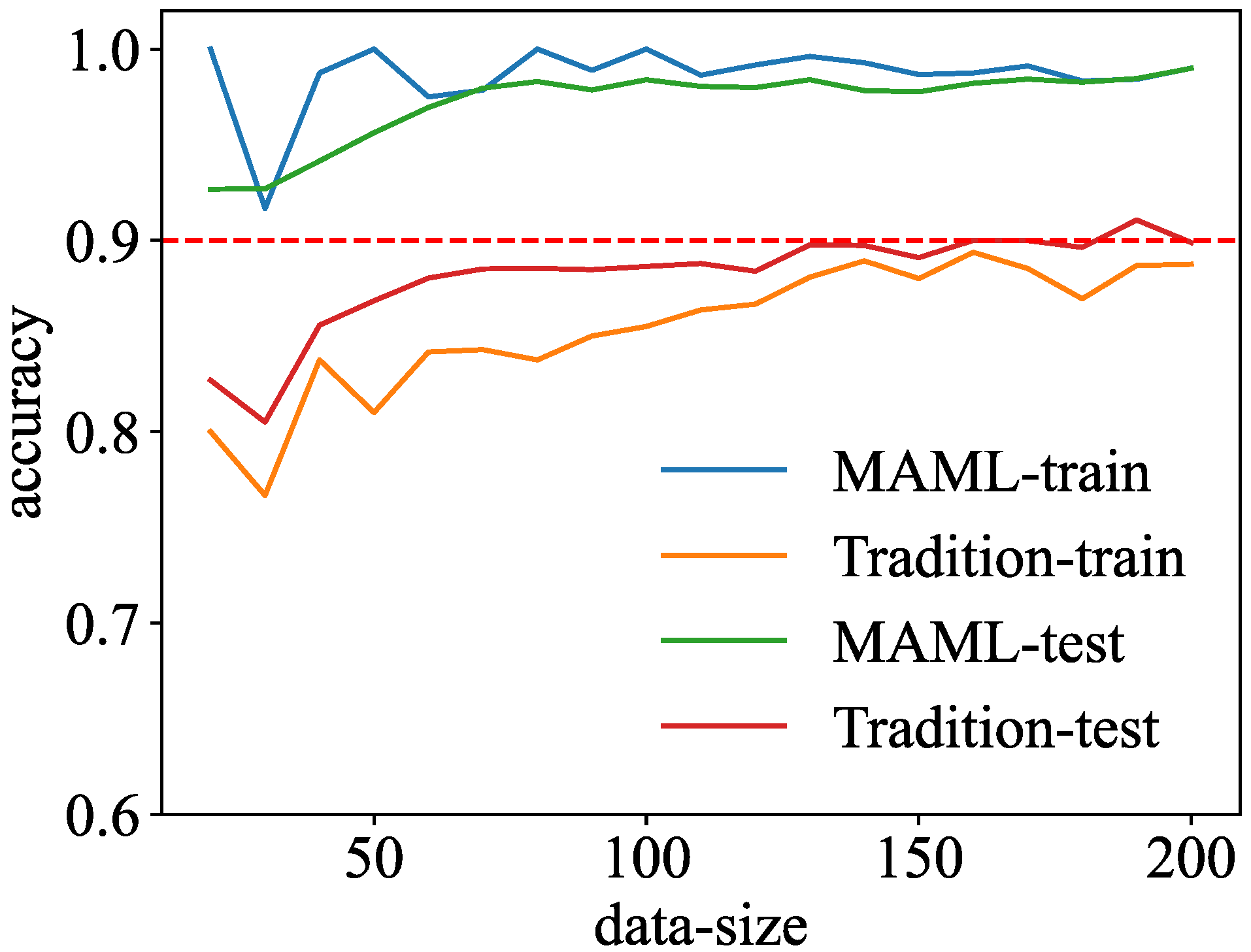
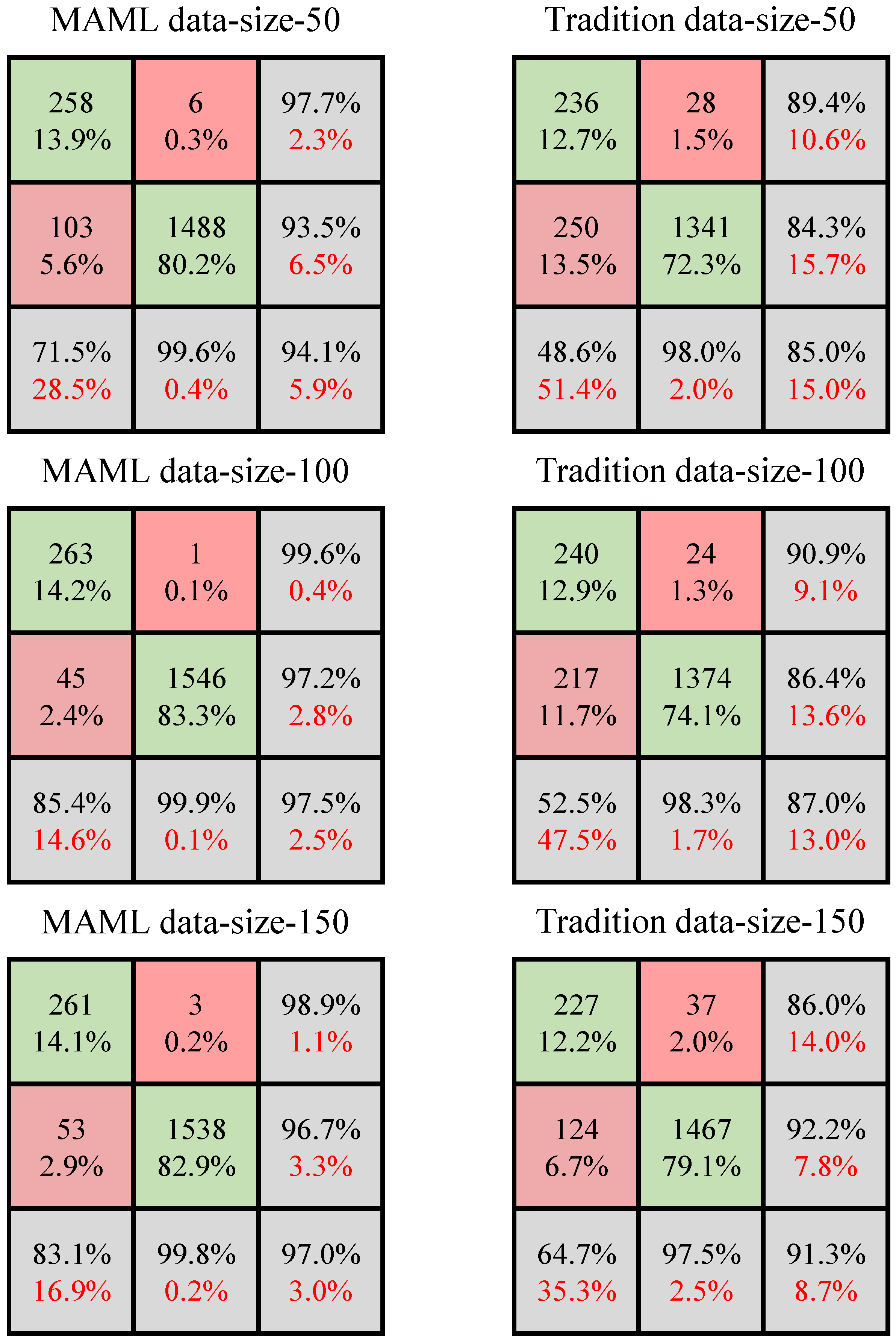
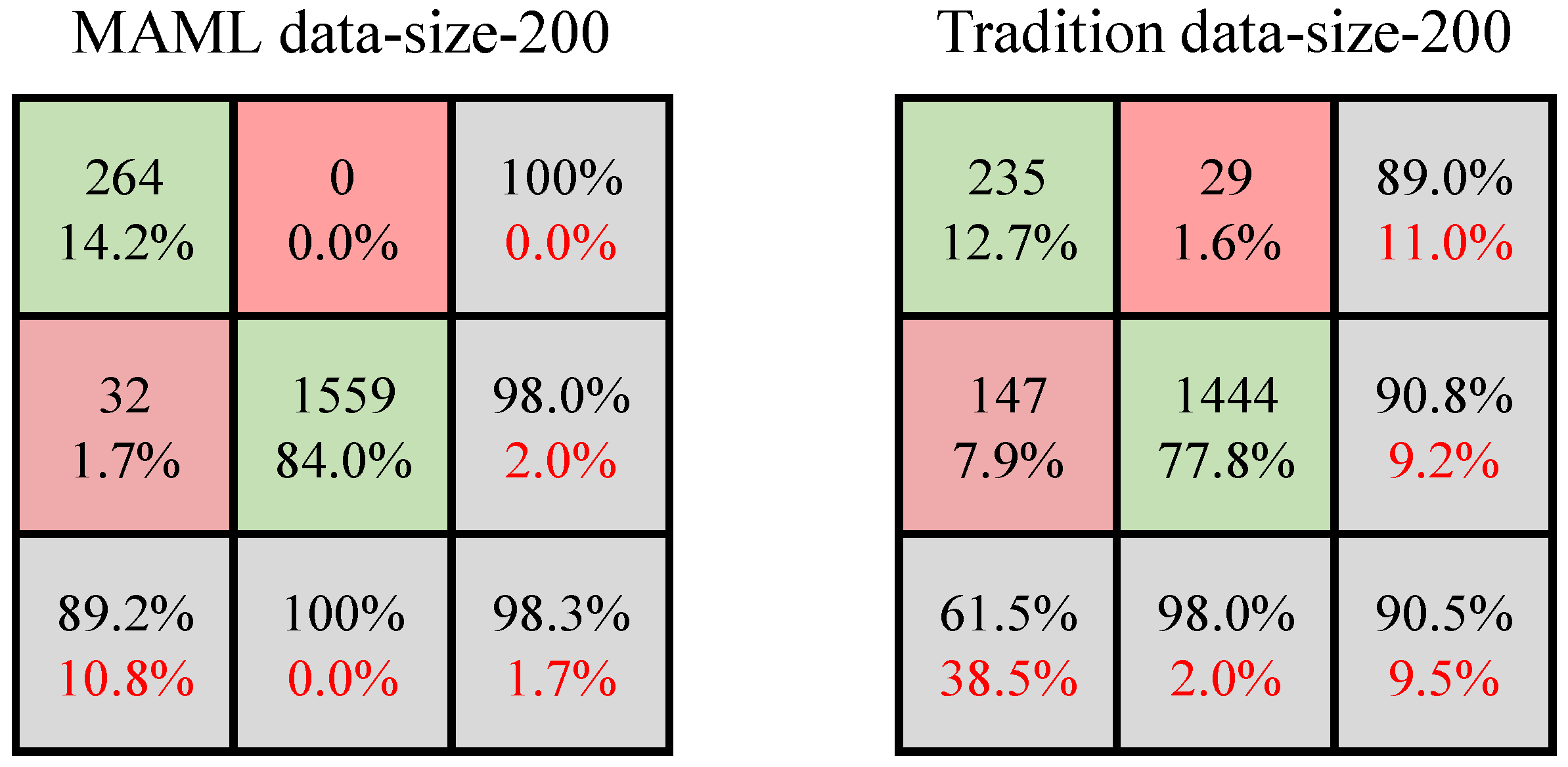
3.4. Performance of MAML-ANN
- (1)
- Comparison between MAML-ANN and traditional ANN
- (2)
- Recognition speed
4. Discussion
5. Conclusions
Author Contributions
Funding
Institutional Review Board Statement
Informed Consent Statement
Data Availability Statement
Conflicts of Interest
References
- De Azevedo, H.D.M.; Araújo, A.M.; Bouchonneau, N. A review of wind turbine bearing condition monitoring: State of the art and challenges. Renew. Sustain. Energy Rev. 2016, 56, 368–379. [Google Scholar] [CrossRef]
- Tummala, A.; Velamati, R.K.; Sinha, D.K.; Indraja, V.; Krishna, V.H. A review on small scale wind turbines. Renew. Sustain. Energy Rev. 2016, 56, 1351–1371. [Google Scholar] [CrossRef]
- Chen, X.; Yan, R.; Liu, Y. Wind turbine condition monitoring and fault diagnosis in China. IEEE Instrum. Meas. Mag. 2016, 19, 22–28. [Google Scholar] [CrossRef]
- Lau, B.C.P.; Ma, E.W.M.; Pecht, M. Review of offshore wind turbine failures and fault prognostic methods. In Proceedings of the IEEE 2012 Prognostics and System Health Management Conference (PHM-2012 Beijing), Beijing, China, 23–25 May 2012; pp. 1–5. [Google Scholar]
- Liu, W.Y.; Tang, B.P.; Han, J.G.; Lu, X.N.; Hu, N.N.; He, Z.Z. The structure healthy condition monitoring and fault diagnosis methods in wind turbines: A review. Renew. Sustain. Energy Rev. 2015, 44, 466–472. [Google Scholar] [CrossRef]
- Matsui, T.; Yamamoto, K.; Ogata, J. Study on improvement of lightning damage detection model for wind turbine blade. Machines 2021, 10, 9. [Google Scholar] [CrossRef]
- Chen, B.; Zhang, M.; Lin, Z.; Xu, H. Acoustic-based whistle detection of drain hole for wind turbine blade. ISA Trans. 2022; in press. [Google Scholar] [CrossRef]
- Du, Y.; Zhou, S.; Jing, X.; Peng, Y.; Wu, H.; Kwok, N. Damage detection techniques for wind turbine blades: A review. Mech. Syst. Signal Process. 2020, 141, 106445. [Google Scholar] [CrossRef]
- Zhang, C.; Yang, T.; Yang, J. Image recognition of wind turbine blade defects using attention-based MobileNetv1-YOLOv4 and transfer learning. Sensors 2022, 22, 6009. [Google Scholar] [CrossRef]
- Zhang, Y.; Avallone, F.; Watson, S. Wind turbine blade trailing edge crack detection based on airfoil aerodynamic noise: An experimental study. Appl. Acoust. 2022, 191, 108668. [Google Scholar] [CrossRef]
- Wang, L.; Zhang, Z. Automatic detection of wind turbine blade surface cracks based on UAV-taken images. IEEE Trans. Ind. Electron. 2017, 64, 7293–7303. [Google Scholar] [CrossRef]
- Yang, K.; Rongong, J.A.; Worden, K. Damage detection in a laboratory wind turbine blade using techniques of ultrasonic NDT and SHM. Strain 2018, 54, e12290. [Google Scholar] [CrossRef]
- Naderi, E.; Khorasani, K. Data-driven fault detection, isolation and estimation of aircraft gas turbine engine actuator and sensors. Mech. Syst. Signal Process. 2018, 100, 415–438. [Google Scholar] [CrossRef]
- Jiang, S.; Lin, P.; Chen, Y.; Tian, C.; Li, Y. Mixed-signal extraction and recognition of wind turbine blade multiple-area damage based on improved Fast-ICA. Optik 2018, 179, 1152–1159. [Google Scholar] [CrossRef]
- Su, Y.; Meng, L.; Kong, X.; Xu, T.; Lan, X.; Li, Y. Small sample fault diagnosis method for wind turbine gearbox based on optimized generative adversarial networks. Eng. Fail. Anal. 2022, 140, 106573. [Google Scholar] [CrossRef]
- Liu, J.; Qu, F.; Hong, X.; Zhang, H. A small-sample wind turbine fault detection method with synthetic fault data using generative adversarial nets. IEEE Trans. Ind. Inform. 2019, 15, 3877–3888. [Google Scholar] [CrossRef]
- Guo, Y.; Zhong, L.; Qiu, Y.; Wang, H.; Gao, F.; Wen, Z.; Zhan, C. Using ISU-GAN for unsupervised small sample defect detection. Sci. Rep. 2022, 12, 11604. [Google Scholar] [CrossRef]
- Hassani, S.; Mousavi, M.; Gandomi, A.H. Structural health monitoring in composite structures: A comprehensive review. Sensors 2021, 22, 153. [Google Scholar] [CrossRef] [PubMed]
- Teng, W.; Ding, X.; Tang, S.; Xu, J.; Shi, B.; Liu, Y. Vibration analysis for fault detection of wind turbine drivetrains—A comprehensive investigation. Sensors 2021, 21, 1686. [Google Scholar] [CrossRef]
- Antoniadou, I.; Dervilis, N.; Papatheou, E.; Maguire, A.E.; Worden, K. Aspects of structural health and condition monitoring of offshore wind turbines. Philos. Trans. A Math. Phys. Eng. Sci. 2015, 373, 20140075. [Google Scholar] [CrossRef] [Green Version]
- Tsai, T.C.; Wang, C.N. Acoustic-based method for identifying surface damage to wind turbine blades by using a convolutional neural network. Meas. Sci. Technol. 2022, 33, 085601. [Google Scholar] [CrossRef]
- Patange, A.D.; Jegadeeshwaran, R.; Bajaj, N.S.; Khairnar, A.N.; Gavade, N.A. Application of machine learning for tool condition monitoring in turning. Sound Vibrat. 2022, 56, 127–145. [Google Scholar] [CrossRef]
- Jatakar, K.H.; Mulgund, G.; Patange, A.D.; Deshmukh, B.B.; Rambhad, K.S. Multi-point face milling tool condition monitoring through vibration spectrogram and LSTM-autoencoder. Int. J. Perform. Eng. 2022, 18, 570. [Google Scholar] [CrossRef]
- Zhang, Y.; Cui, Y.; Xue, Y.; Liu, Y. Modeling and measurement study for wind turbine blade trailing edge cracking acoustical detection. IEEE Access 2020, 8, 105094–105103. [Google Scholar] [CrossRef]
- Finn, C.; Abbeel, P.; Levine, S. Model-agnostic meta-learning for fast adaptation of deep networks. In Proceedings of the 34th International Conference on Machine Learning (ICML 2017), Sydney, Australia, 6–11 August 2017; Volume 70, pp. 1126–1135. [Google Scholar]
- Goodfellow, I.; Bengio, Y.; Courville, A. Deep Learning; MIT Press: London, UK, 2016. [Google Scholar]
- Janeliukstis, R. Continuous wavelet transform-based method for enhancing estimation of wind turbine blade natural frequencies and damping for machine learning purposes. Measurement 2021, 172, 108897. [Google Scholar] [CrossRef]
- Tong, R.; Li, P.; Lang, X.; Liang, J.; Cao, M. A novel adaptive weighted kernel extreme learning machine algorithm and its application in wind turbine blade icing fault detection. Measurement 2021, 185, 110009. [Google Scholar] [CrossRef]
- Zhou, Z.H. Machine Learning, 1st ed.; Springer: Singapore, 2021. [Google Scholar]
- Deo, T.Y.; Patange, A.D.; Pardeshi, S.S.; Jegadeeshwaran, R.; Khairnar, A.N.; Khade, H.S. A white-box SVM framework and its swarm-based optimization for supervision of toothed milling cutter through characterization of spindle vibrations. arXiv 2021, arXiv:2112.08421. [Google Scholar]


| Location | Placement | Height (m) |
|---|---|---|
| A | behind | 5 |
| B | behind | 1.5 |
| C | front | 5 |
| D | front | 1.5 |
| E | side | 5 |
| F | side | 1.5 |
| Hyperparameters | Numerical |
|---|---|
| learning rate | 0.0005 |
| k-shot | 2 |
| q-shot | 5 |
| batch size | 4 |
Publisher’s Note: MDPI stays neutral with regard to jurisdictional claims in published maps and institutional affiliations. |
© 2022 by the authors. Licensee MDPI, Basel, Switzerland. This article is an open access article distributed under the terms and conditions of the Creative Commons Attribution (CC BY) license (https://creativecommons.org/licenses/by/4.0/).
Share and Cite
Zhu, Y.; Liu, X.; Li, S.; Wan, Y.; Cai, Q. Wind Turbine Blade Defect Detection Based on Acoustic Features and Small Sample Size. Machines 2022, 10, 1184. https://doi.org/10.3390/machines10121184
Zhu Y, Liu X, Li S, Wan Y, Cai Q. Wind Turbine Blade Defect Detection Based on Acoustic Features and Small Sample Size. Machines. 2022; 10(12):1184. https://doi.org/10.3390/machines10121184
Chicago/Turabian StyleZhu, Yuefan, Xiaoying Liu, Shen Li, Yanbin Wan, and Qiaoqiao Cai. 2022. "Wind Turbine Blade Defect Detection Based on Acoustic Features and Small Sample Size" Machines 10, no. 12: 1184. https://doi.org/10.3390/machines10121184