Article

Real-Time Neural Classifiers for Sensor and Actuator Faults in Three-Phase Induction Motors

by
Oscar D. Sanchez
,
Gabriel Martinez-Soltero
,
Jesus G. Alvarez
and
Alma Y. Alanis
*,†
University Center of Exact Sciences and Engineering, University of Guadalajara, Guadalajara 44100, Jalisco, Mexico
*
Author to whom correspondence should be addressed.
Current address: Marcelino Garcia Barragan 1421, Guadalajara 44430, Jalisco, Mexico.
Machines 2022, 10(12), 1198; https://doi.org/10.3390/machines10121198
Submission received: 1 October 2022 / Revised: 28 November 2022 / Accepted: 2 December 2022 / Published: 10 December 2022
(This article belongs to the Section Machines Testing and Maintenance)

Abstract

:
The main steps involved in a fault-tolerant control (FTC) scheme are the detection of failures, isolation and reconfiguration of control. Fault detection and isolation (FDI) is a topic of interest due to its importance for the controller, since it provides the necessary information to adjust and mitigate the effects of the fault. Generally, the most common failures occur in the actuator or in sensors, so this article proposes a novel model-free scheme for the detection and isolation of sensor and actuator faults of induction motors (IM). The proposed methodology performs the task of detecting and isolating faults over data streams just after the occurrence of the failure of an induction motor (IM), by the occurrence of either disconnection, degradation, failure, or connection damage. Our approach proposes deep neural networks that do not need a nominal model or generate residuals for fault detection, which makes it a useful tool. In addition, the fault-isolation approach is carried out by classifiers that differentiate characteristics independently of the other classifiers. The long short-term memory (LSTM) neural network, bidirectional LSTM, multilayer perceptron and convolutional neural network are used for this task. The proposed sensors’ and actuator’s fault detection and isolation scheme is simple. It can be applied to various problems involving fault detection and isolation schemes. The results show that deep neural networks are a powerful and versatile tool for fault detection and isolation over data streams.

1. Introduction

In recent years, fault-tolerant control systems have attracted the interest of academics, professionals and industry due to the increasing complexity of the systems to be controlled and different system components that cause uncertainties, threats and disturbances, among other phenomena of stress [1,2].
Fault-tolerant control (FTC) schemes are used to mitigate the effects caused by faults. Their relevance lies in the fact that this approach provides security and reliability, maintaining the overall performance and stability of the system despite system failures or breakdowns. In general, the FTC approach is divided into two phases [3,4]:
(1)
Fault detection and isolation (FDI): its objective is to process input/output data, in order to detect the existence of a fault, to isolate it from other faults or alterations of the system [5];
(2)
Tolerant control algorithm: its objective is to adjust the controller to compensate for the effect of a fault, based on the information provided by the fault detector [3].
This work deals with the first task concerning the FTC, which is the identification and detection of existing faults also called the diagnostic problem. This problem can be divided into two stages: a failure-detection stage and fault-isolation stage. In the failure-detection stage, it determines if a failure has occurred, in addition to distinguishing the moment in which the system has been subject to a failure [6]. On the other hand, the fault-isolation stage focuses on determining the component in which the fault originated [6].
Mainly, there are three kinds of faults in induction motors: actuator faults, machine faults and sensor failures. In industrial applications, the FTC for sensor failures is crucial, since the sensors keep under observation the system state variables—some of the components with the greatest potential for failure. In fact, as mentioned in [7], analyzing the observations made by the sensors is a challenging task. Additionally, the actuators represent a connection between the control algorithm and the system, so if there is a fault in the actuator, the operating capacity is reduced compared to normal operation. Among the principal applications of fault detection and isolation is to guarantee reliability and safety, such as for high-speed trains [7].
In general, FDI approaches are classified as model-free and model-based paradigms. Model-based schemes use redundancy from mathematical models of the system. However, it has the disadvantage that it ignores variable parameters and noise. Furthermore, it is not always possible to obtain the nominal model of the system. Among the works that use model-based FDI schemes, we can mention observers based on the Kalman filter, adaptive observers and sliding mode observers [8,9,10,11,12,13,14]. In contrast, model-free approaches include techniques that do not depend on nominal models of the underlying system. Most of the model-free FDI schemes published were designed based on artificial intelligence approaches [1,15,16]. As mentioned in the work published in [17], the traditional approach to detecting and diagnosing faults is carried out in five steps. These are data acquisition, data processing, feature extraction, dimensional reduction and classification. This implies that finding the right techniques at each step is of the utmost importance and a process of trial and error is mandatory. Due to this, different works use unique approaches to address the each particular application.
For example, in [18], a distributed system for the detection and diagnosis of sensor failures is proposed using an automatic encoder that reduces the dimensions of the input signal, which serves as input to a support vector machine (SVM)) for classification as normal or defective. In [19], two model-based fault diagnosis methods are proposed to estimate the residual current dynamics. In the first method, a differential algebraic estimation of the failure dynamics is performed; in the second, a combination of an algebraic approach and the robust integral sign of error (RISE) observer are used. Then, upon detecting that a fault has occurred, it goes to a logic-based decision unit to identify the faulty sensor. In another recent work [20], the multi-headed 1D convolutional neural network (1D CNN) was used to detect and diagnose six different types of faults in an electric motor using two accelerometers; the results shown are from offline tests, so real-time tests were ruled out. Regarding detection and diagnosis of faults in real time, we can mention [21], which presents a machine learning approach. The study involved data from a 3D machine simulation system with faulty and non-faulty conditions. The main disadvantage is that this model needs 70% of data for training and only 30% for testing. This work was limited to fault detection only and did not take fault isolation into account.
In another work [22], an FDI methodology that allows fault diagnosis for sensors and actuators proposes the modeling and inversion of non-linear systems using recurrent neural networks which are used to build predictive models and generate residuals. It is sensitive to a set of failures and insensitive to the rest, which generates the classification of the failure; nevertheless, the online implementation was ruled out. Deep neural networks do not need a combination of techniques at each step; rather, deep layers are generated for feature learning. In this sense, fault detection and isolation tasks can be based on artificial neural networks (ANNs). However, there are not many results regarding online fault detection and isolation with ANNs. Moreover in [23], an ANN was used along with a deterministic finite-state automaton to detect and isolate the faults and anomalies in the manufacturing of programmable logic controllers (PLCs). To automate detection of the failures in the control process, the ANN is in charge of the anomalies that do not affect much the state transition behavior of the PLC. Similarly, reference [24] used an MLP network as an autoregressive model with exogenous inputs, having the ability to model the dynamic system based on time series data. Hybrid models such as [25] use a combination of techniques. In the case, for preprocessing the data, the wavelet packet transform, and then, they are passed as the input into an autoencoder to extract the fault features, followed by the equilibrium optimizer algorithm and long short-term memory for fault detection and classification.
Deep neural networks have been used for classification tasks in different areas, such as the medical field for early detection of diseases, including Parkinson’s disease [26] and heart faults [27], and detection of faults in sensors of medical equipment [28] employing an LSTM. In industry, they are normally used for the detection of faults in equipment to make the production efficient [29]; in the detection of incorrect assemblies, avoiding the cost of delivering an unusable finished product [30]; and for improving the maintenance with early detection of faulty machinery gears [31]. The electrical field needs the detection of faults in circuits or motors, which could be the sources of accidents, using the current, vibration or voltage as input for the model [31,32,33].
In general, the aforementioned works explored offline classification. In fact, an interesting review shows exhaustive research about fault detection and isolated work for traction systems in high-speed trains [7]. Here, a compilation of numerous papers with different methodologies for diagnosis and detection is presented, among which are mentioned signal analysis-based, model-based and data-driven (or model-free) methods. As mentioned in this paper, strategies developed for the use of fault-tolerant controllers are a topic of interest for researchers; however, there are not many works related to FDI schemes with the purpose of being used in controllers. However, for real-time applications, it is necessary to have a reliable classifier that works online along with a fault-tolerant controller. This paper proposes a novel methodology for the online diagnosis of actuator and sensor faults in an induction motor test bench, only with data measured without knowledge of the nominal model or prior knowledge other than the data with which the ANN were trained. This methodology was implemented with four deep neural network architectures, and their performances were tested with experimental data. The main contributions are:
  • Four online neural classifiers are proposed to deal with actuator and sensor faults;
  • Classifiers are tested online with experimental data;
  • A real-world problem for actuator and sensor fault classification is included;
  • A detailed comparative analysis was performed for the four proposed classifiers to deal with actuator and sensor faults.
  • Proposed methodology can be easily extended to different real-world fault diagnosis and classification problems.
This paper is organized as follows, Section 2, includes a review of the induction motor used to test the proposed methodology. Then, Section 3 includes an explanation of the neural networks proposed to deal with faults classification. After that, in Section 4, the proposed methodology is presented for the detection and isolation fault scheme. In Section 5, the results are presented, along with the discussion about obtained results, and finally, in Section 6, conclusions and future work are stated.

2. Review of the Analyzed System

Rotatory induction motors (RIM) are widely used in multiple types of applications, e.g., in electric vehicles, electric elevators, compressors, robotics, machine tools and the aerospace industry, among others. RIM uses different approaches for control. One of the most used is using the α β coordinates; due to this model being a coordinate system that is based on α β axes, the base is static, so the transformed voltage vector rotates at the power supply frequency and its components are projected on α β axes. Figure 1 represents the test bench configuration used. Measured signals were obtained from voltage, current and position sensors, and data acquisition was performed with a DSPACE©DS1104 board. Then, such information was processed and classified according to the four online neural classifiers proposed in this work. The isolation task was performed through the control algorithm using the output D/A channels.
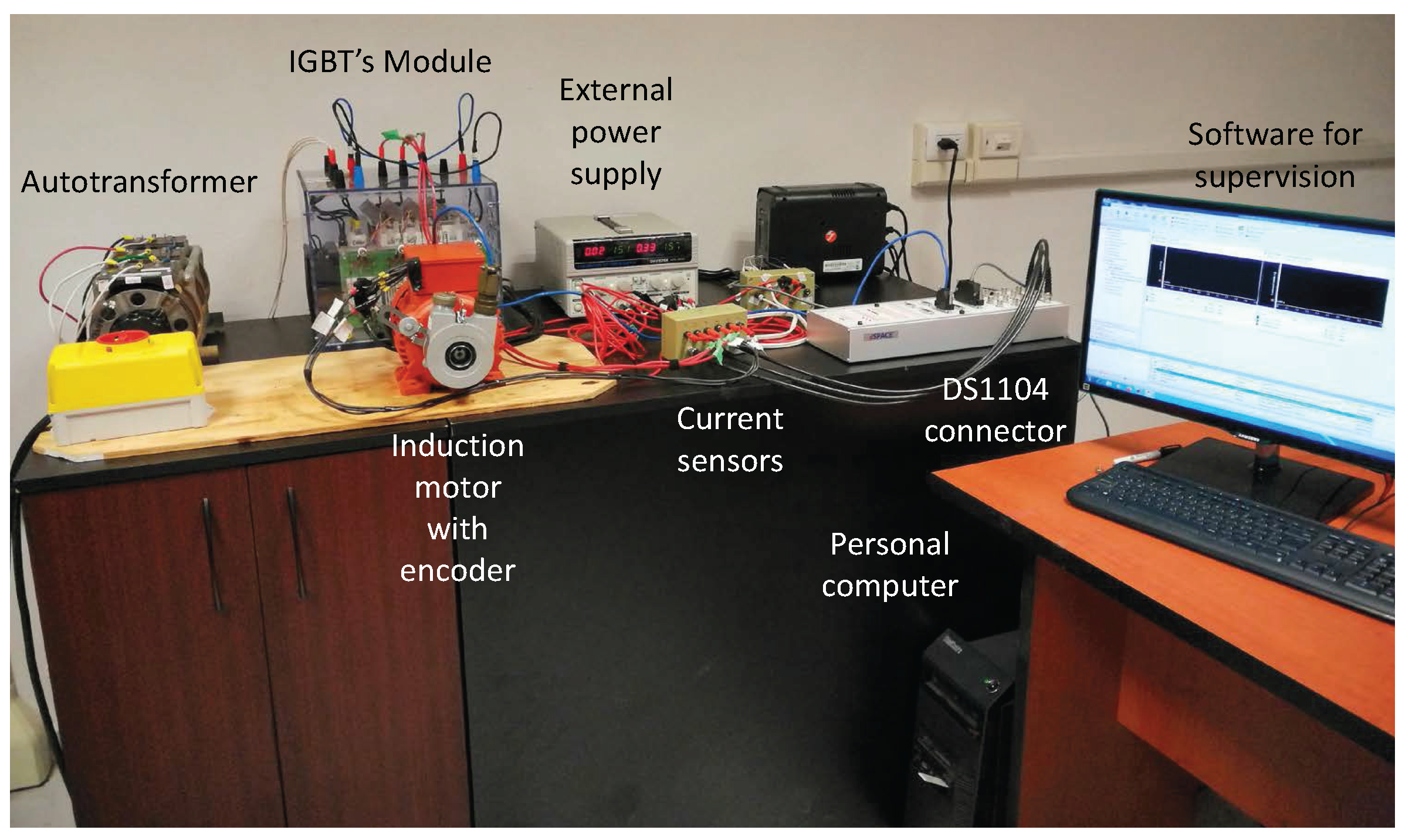
The proposed fault detection and isolation methodology was applied to a three-phase induction motor through the test bench shown in Figure 2, which included the following components: a three-phase induction motor, an autotransformer, a DSPACE©DS1104 board, current sensors, an IGBT module, an external power supply, a TTL-CMOS converter and a computer for programming and supervision. Data tests were acquired through the DSPACE©DS1104 board, using Hall effect sensors and the encoder to measure currents and position, respectively. The experimental faults were introduced via software in order to test the applicability of the proposed methodology.
FDI model-based schemas use observers to monitor the sensors in cases of failures. Then, observers generate a difference to compare it with a threshold and decide if the sensors are failing or not [8]. However, observers rely on a nominal model of the system, which can neglect time-varying parameters and noise and rely on measurements made by fault-prone sensors (voltages, currents and rotor position). For this work, we used deep neural networks which are capable of learning the characteristics of the sensors when they are healthy and characteristics when they show faults without the need for the nominal model.

3. Deep Neural Networks

For real-world applications, there is a need to develop fault diagnosis methods with the ability to analyze large amounts of data for automatic fault detection accurately and quickly. Frequently, the fault detection for the IM is based on observers; however, its main disadvantage lies in its great dependence on precise mathematical models corresponding to the system. This is not completely effective in real applications because the system’s parameters often vary during the process, and the disturbances are unknown, which can cause false alarms [34]. However, neural networks that have been adopted for intelligent fault diagnosis have shallow architectures [35]. This limits the ability of ANNs to learn complex nonlinear relationships, so it is necessary to establish a deep architecture network for this purpose.
Deep neural networks contain multiple layers of nonlinear operations for handling complex structures. These layers are connected to the previous one, in such way that the parameters (weights) are adjusted to abstract representations of real applications [36]. DNNs capture complex functions through training of the multiple levels of abstraction, with only the knowledge of raw sensor data, since the neural network can learn the characteristics of the sensor both in failure conditions and in a healthy state.
DNNs have attracted the attention of researchers in different fields and have shown to be very effective for complex real-world problems such as classification, image processing [37], speech processing [38], language models [39] and sequential data [40]. However, deep neural networks are relatively new to the task of detecting and isolating system faults. However, DNNs have the potential to overcome the sensor failure diagnostic deficiencies of the current methods due to their deep architectures. The use of DNN will help to develop better and more reliable fault diagnosis systems.
In this work, we propose four networks for classification of sensor and actuator faults of an induction motor, in a fast and precise way. These are multilayer perceptron neural network, long short-term memory (LSTM), bidirectional LSTM and convolutional neural network methods. All of them are described below.

3.1. Multilayer Networks

The multilayer perceptron (MLP) neural network is one of the most influential network models and has been widely used in various problems [41,42]. MLP gained popularity in classification problems because it is an efficient, flexible neural network [42]. The MLP structure consists of an input layer, one or more hidden layers and an output layer. Hidden layers contain several nodes. These nodes are connected with other nodes of contiguous layers through weights.
The sum of the m neurons in the hidden layer multiplied by their nodes of input u n are multiplied by the connection weights. W generates the output of the neural network y p , as described by the following Equation (1):
y p = σ ( W n m σ ( W n n u n + b 1 ) + b 2 )
where m represents the number of neurons, u n is the input, σ is the activation function, W n n represents the weight matrix of the first layer and W n m represents the weight matrix of the second layer.

3.2. Long Short-Term Memory Recurrent Neural Network

A popular recurrent neural network (RNN) in the field of deep learning is the LSTM proposed in [40]. The RNN presents the difficulty of learning long-term dependencies, but the LSTM network was proposed with the aim of solving said long-term dependency problem through the introduction of an input gate, an output gate and a forget gate [43]. The three gates control the memory of past states. Among the works that have used the LSTM as a classifier, we can name [44,45,46]. LSTM is implemented by Equations (2)–(7):
i t = σ ( W x i x t + W h i h t 1 + W c i c t 1 + b i )
f t = σ ( W x f x t + W h f h t 1 + W c f c t 1 + b f )
C ˜ t = t a n h ( W x c x t + W h c h t 1 + b c )
C t = f t C t 1 + i t C ˜ t
o t = σ ( W x o x t + W h o h t 1 + W c o C t + b o )
h t = o t t a n h ( C t )
where i is the input gate, f is the forget gate, o is the output gate, C is the activation cell, σ is the logistic sigmoid function and h t the hidden state vector as a representation of the output gate value between −1 and 1. b i , b f , b c , b o are the learned biases. W are weight matrices; that is, W x i , W x f , W x c , and W x o are the weights that connect the input layer with the input gate, forget gate, activation cell and output gate, respectively. W h i , W h f , W h c , and W h o connect the hidden layer with the input gate, forget gate, activation cell and output gate. W c i , W c f , and W c o connect the activation cell with the input, forget and output gates. Finally, t a n h scales the values into the range of −1 to 1.

3.3. Bidirectional LSTM

The bidirectional recurrent neural networks (BRNNs) proposed in [47] divide the state of the neurons of the RNN into two parts, the forward state (positive direction) and the backward state (negative direction). Each is independent from the other [47]. Then, the bidirectional structure is applied to the LSTM, allowing LSTM cells to access the forward and backward states. The Bi-LSTM is implemented by Equations (8)–(10):
h t = H ( W x h x t + W h h h t 1 + b h )
y t = W h y h t + W h y h t + b y
where h is the hidden state of the LSTM cell, h t is the hidden layer from the forward state and h t is the hidden layer for the backward state. Then, forward and backward states are combined to produce the output y t . H is the activation function. The weight matrices W are: W x h are the weights that connect the input layer and the hidden layer; W h h connect the hidden layer and the previous hidden states; W h y connect the hidden layer and the output; finally, b h , b h and b y , represent the bias vectors.

3.4. Convolutional Neural Network

There are several deep neural network architectures, including the so-called convolutional neural network (CNN), whose advantages are weight sharing and minimized computation in comparison with a regular neural network. The CNN applications have focused on object recognition [48], image classification and time series [49,50] and have been used for fault detection in recent years [51,52]. The graphical representation of applying a CNN for time series classification is shown in Figure 3.

4. Proposed Method Based on Deep Neural Networks

Current real-time requirements for the immediate processing of data, in addition to the variation of behavior patterns in the data observed by the sensor over time, mitigate the effectiveness of conventional machine learning methods. In addition, uncertainties, non-linear elements and the variability of the nature of the sensor data, which serve as valuable information in monitoring processes to capture the relationship between time series data, require a novel approach to fault classification. These approaches should be computationally efficient and have high levels of prediction accuracy and precision.
Among the main contributions of this work is generating accurate and reliable model-based FDI schemes using deep neural networks capable of being implemented in model-free fault-tolerant control schemes. Thus, we can model the system with faulty sensors and an actuator such as in Equation (11).
x ¯ ( t + 1 ) = F ( x ¯ ( t ) , u ¯ ( t ) ) + d ( t )
y ( t ) = C x ¯ ( t )
where x R n is the system state vector, u R m , F R n × R m R n is a nonlinear function, C R p × m is the output matrix and d R n is the perturbation vector. We can rewrite (11) in its component-wise form:
x ¯ i ( t + 1 ) = F i ( x ¯ ( t ) , u ¯ ( t ) ) + d i ( t ) i = 1 , 2 , , n
The sensor and actuator failures are defined as:
x ¯ ( t ) = ρ i ( x i ( t ) , δ i ( t ) )
u ˜ ( t ) = ϕ i ( u i ( t ) , δ i ( t ) )
where δ i is the vector of uncertainties; ρ i and ϕ i are nonlinear functions considered unknown but bounded and represent the loss of sensor and actuator efficiency caused by external inputs being either unmeasurable, biased, drifted or showing loss of precision over time t i * . Then, x i ( t ) is considered measurable, and its measure is x ¯ i ( t ) . A Schematic representation of (11) can be appreciated in Figure 4.
For FDI purposes, the intrinsic values of x ¯ and u ¯ vectors of the internal dynamics of system (11) can result in only two possible outcomes: faulty or healthy. Then, this can be considered as a classification problem described by
ρ i ( x i ( t ) , δ i ( t ) ) = f a i l u r e , ρ i ( * ) S n o n - f a i l u r e , ρ i ( * ) S
Similarly,
ϕ i ( u i ( t ) , δ i ( t ) ) = f a i l u r e , ϕ i ( * ) S n o n - f a i l u r e , ϕ i ( * ) S
where S is the subset of all possible fault modes. Then, the subset S is considered only partially known due to the nonlinear system being difficult to entirely define.
If the full state x ( t ) of the system is available and there exists a data structure with the dynamics of (16) and (17) that can be identified as features in a time series, then we can say that it is possible to identify a fault scenario in the system by combining all signal inputs in a multivariate time series.
For this work, we consider the deep networks described above to perform the classification task (16) and (17), so the problems of fault detection and isolation are separated into two stages: the signal isolation stage and the fault classification stage. The methodology is described below.

4.1. Fault-Isolation Logic

The data set obtained by the actuator or sensors can be considered as a time series that has a relationship between current and past data, so it can corroborate trends. We can define a time series as a vector X made up of real values measured by failure-prone sensors x ¯ ( k ) , as defined in (18):
X = [ x ¯ ( 0 ) , x ¯ ( 1 ) , , x ¯ ( n ) ]
The size of the vector corresponds to the number of samples observed, n. Then, there are different ways of approaching the FDI problem: on the one hand using multivariate time series (data collected from measurements of multiple sensors or variables) classification techniques, and on the other univariate time series (data collected from measurements of the same variable).
It should be noted that in order to detect a failure in time, each sample must be monitored as it is obtained from the sensors and the actuator. For multivariate time series, the classification problem can be addressed through dynamic time warping and features extracted from time series data [53]. The main disadvantage of these methods is the computational cost, which complicates online classification. Among the works that have used multivariate time series data for classification tasks are [44,54,55,56,57,58].
Additionally, fault detection and diagnosis schemes are limited to recognizing the existence of a fault; however, for the purposes of use in fault-tolerant controllers, it is also necessary to isolate the fault. To this end, data-driven schemes use neural networks in the fault-isolation stage. However, this approach for fault detection and isolation rules out closed-loop control purposes [23,24].
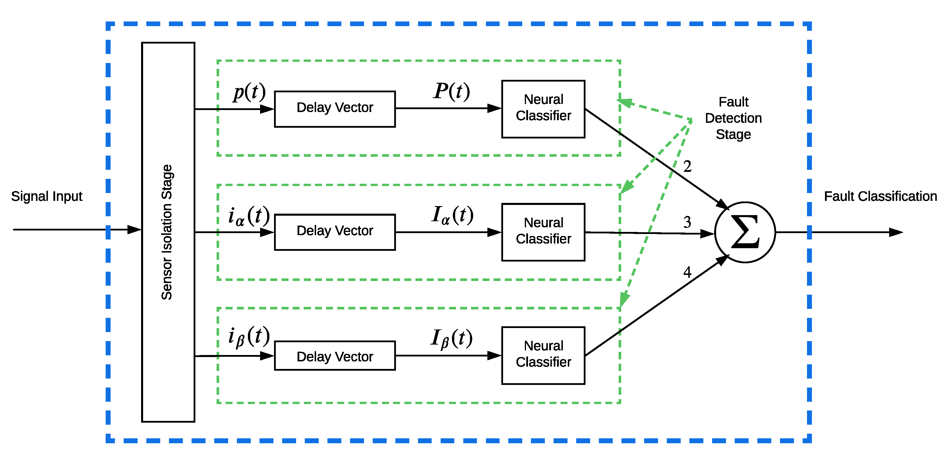
Thus, to reduce the computational cost, it is more convenient to deal with univariate time series, and for model-free FDI schemes, it implies less complex architectures compared to those used for multivariate time series. In this way, to isolate the fault (fault-isolation stage), the different signals are separated. Then, each signal is considered a channel. Each of these channels has a block of a neural classifier that learns the corresponding characteristics individually.
Thus, N different univariate X ( k ) time series, such as Equation (18), can be seen as multivariate time series consisting of X = [ X ( 1 ) , X ( 2 ) , , X ( N ) ] . Then, the data set D = { ( X ( 1 ) , Y ( 1 ) ) , ( X ( 2 ) , Y ( 2 ) ) , , ( X ( N ) , Y ( N ) ) } is a collection where X ( k ) is a time series univariate and Y ( k ) is its class label vector. The length of Y ( k ) corresponds to the number of classes i, where each element j [ 1 , k ] is equal to 1 if the class of X ( k ) is j and 0 otherwise.

4.2. Fault-Detection Logic

A univariate time series presents the problem of incorporating information because only one signal is considered available. In the case of deep neural networks, the context and the information provided are of great importance. Thus, incorporating context for neural networks in univariate time series it can be done in two ways: one can use recursive connections to model the time flow directly or collect inputs in overlapping time windows [44].
The extraction of information from past observations is known as sliding window or time delay embedding. This approach has been used in understanding the nature of attractors of dynamic systems in addition to verifying nonlinearity and chaotic behavior in the dynamics of the electroencephalogram, electrocardiogram and electromyogram [59].
Here, the sliding window implemented online is explored. For this, We consider X as a function defined on an interval of the observed time series { x ¯ ( 0 ) , x ¯ ( 1 ) , , x ¯ ( t ) } . Thus, the sliding-window embedding X ( t ) is a delay vector generated by extracting local information of the time series defined up to the current time t. This is Equation (19).
X ( t ) = [ x ¯ ( t ( d 1 ) ) , , x ¯ ( t 1 ) , x ¯ ( t ) ]
where { 1 , 2 , , d 1 } are the sampling lag and d is the array dimension. Then, the vector X ( t ) is the input to the neural networks to predict the class Y ( t ) . The graphic representation is shown in Figure 5. This process is repeated for each new sample that is observed.
Different dimensions of the delay vector were tested to find the appropriate number of dimensions that reduces the classification error according to the complexity of the signal.

4.3. Architecture of the Proposed NN Classifier

The fault classification problem is addressed for the actuators and sensors of the fault-tolerant control scheme. Our proposal is to separate the FDI into two blocks, one for actuator fault detection and a classification block for system sensors, as shown in Figure 6 and Figure 7, respectively. Then, the observed signals are separated into different channels (isolation stage). These are: p position, i α current, i β current, actuator voltage u α and actuator voltage u β . Delay vectors of dimension d are generated that serve as input to the neural classifiers. The output of the classifier represents the class of the fault it predicts. Figure 6 and Figure 7 represent the configurations used for the online classification of sensors and the actuator signals with the various neural networks. The labels for faults of the sensor block and actuator are shown in Table 1 and Table 2, respectively.
The architecture of the neural networks used for each channel is described below:
  • Position channel neural classifier architecture: For the fault classification of the position sensor, the four proposed neural networks were tested. Each neural network has two inputs, corresponding to the delayed vector [ p ( t 1 ) , p ( t ) ] that is generated to add context to the classification. All neural networks have one output. The hidden layers and neurons for each neural network are as follows: MLP has 2 hidden layers with 20 neurons in each layer; LSTM contains 1 hidden layer with 15 LSTM cells; BiLSTM contains 1 layer with 15 LSTM cells for the forward state and 15 neurons for the hidden backward state layer; finally, the CNN contains 1 convolution + ReLu layer with 20 filters, followed by 1 pooling and 2 dense layers.
  • Current channel neural classifier architecture: In the current sensors, different dimensions are explored for the delay vectors. These are dimension d = 8, the delay vector I α ( t ) = [ i α ( t 7 ) , i α ( t 6 ) , , i α ( t ) ] ; and dimension d = 10, I α ( t ) = [ i α ( t 9 ) , i α ( t 8 ) , , i α ( t ) ] , where t is the current sample. Therefore, the numbers of inputs of the neural networks are 8 and 10, and there is only 1 output. The numbers of hidden layers and neurons are the same as the aforementioned for all inputs for the MLP, LSTM and BiLSTM. The CNN has a convolution + ReLu layer, a pooling layer and two dense fully connected layers; the numbers of filters and neurons per layer are as shown in Table 3:
Table 3. CNN architecture.
InputsConvolution + ReLuDenseDenseOutputs
+ Pooling LayerLayer 1Layer 2
8201401001
10201801001
  • Actuator voltage channel neural classifier architecture: Similarly, for the actuator voltages, the delay vector dimensions of 8 and 10 were used, so the vectors were u ( t ) = [ u ( t ( 7 ) ) , , u ( t ) ] and u ( t ) = [ u ( t ( 9 ) ) , , u ( t ) ] . Since the actuator voltage channel signals are similar to the current channel signals, the same architecture was used.

5. Results

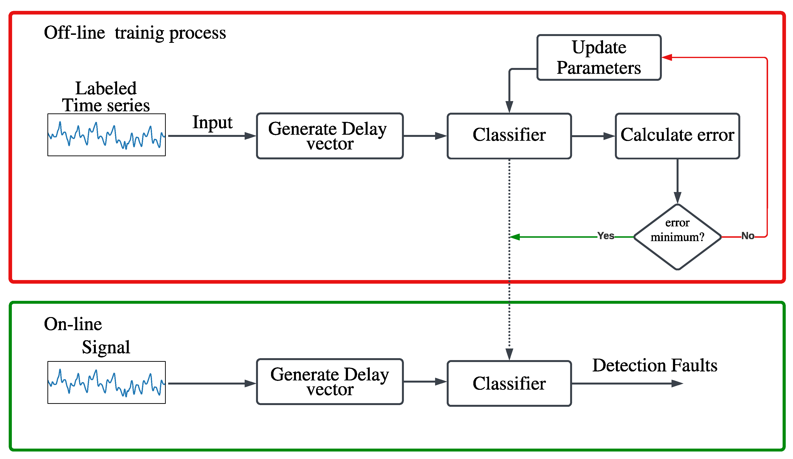
Figure 8 shows the training that was carried out offline with completely different data than the test data. It should be noted that the sliding windows were generated at different dimensions in order to find the best number of dimensions regarding the classification error. For its part, the real-time implementation used the adjusted parameters in the training of the neural networks.
The results were obtained using the four neural networks with their respective architectures mentioned above. The neural classifiers were trained individually for each channel; 20,000 samples were used. Half of the samples did not present faults, and the other half presented faults. Figure 9 represents the data used for validation of the sensor block, and Figure 10 represents the data used for validation in the actuator block.
Figure 9 shows Channels 1, 2 and 3. A total of 100,000 samples were used in the validation. The position channel shows failure at samples 70,023–75,032, and the current channel i α shows failure from sample 20,002 to sample 25,005. Finally the current channel i β shows failure from sample 50,006 to sample 55,011. The actuator data are shown in Figure 10, for Channels 4 and 5. The voltage u α channel shows a fault at 53,008 to 58,013. For its part, the voltage u β presents the fault in the interval 60,013–65,022.
To compare the different neural classifiers’ performances, we used classification accuracy (CA), the confusion matrix (CM) and the graphs of the ROC curves (receiver operating characteristic curve). The classification precision equation indicates the relationship between the number of correct predictions and the total number of samples, which is obtained by Equation (20).
A c c u r a c y = T r u e p o s i t i v e T r u e p o s i t i v e + F a l s e p o s i t i v e
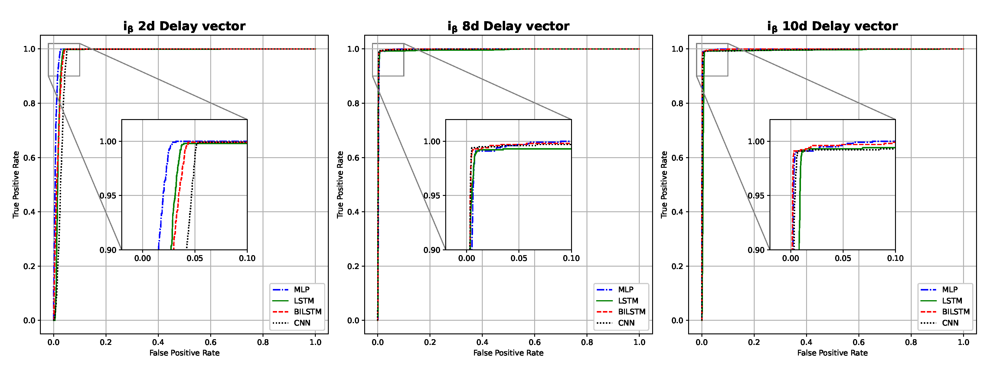
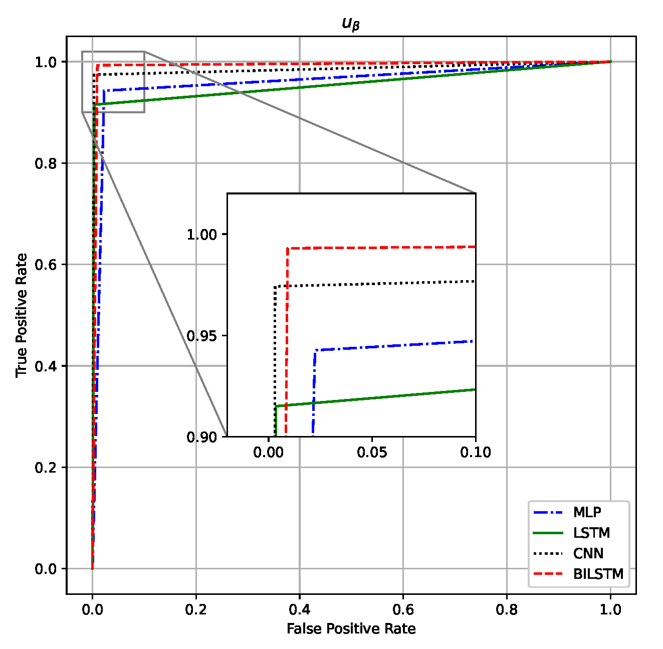
The ROC curve is used to evaluate the discriminative ability of two or more methods to differentiate between classes, and different cutoff points to compare the rates of true positives and false positives. The line where true positives equal false positives means random sorting performance. The higher the line on the ROC chart, the better the classification performance. The classification method is capable of separating all the positive cases from the negative ones if the curve passes through the point of true positives equal to 1 and false positives equal to 0 [60].
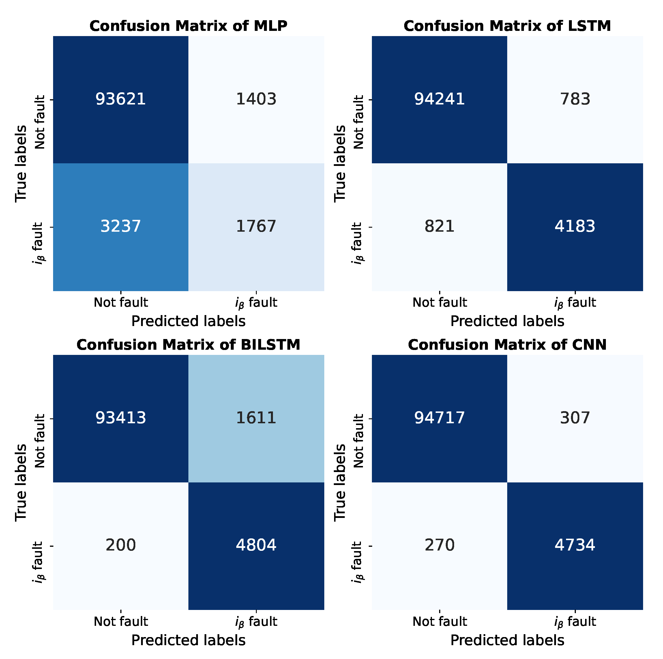
The confusion matrix is a detailed summary of the classification results. It takes into account true positives (positive predictions that were correct), true negatives (predictions of the negative class that were correct), false negatives (cases assigned to the negative class that were incorrectly classified) and false positives (negative cases that were incorrectly classified as positives).
The ROC curves of the four neural networks for different channels are shown in Figure 11, Figure 12, Figure 13, Figure 14 and Figure 15. The CA and average time that each neural network takes to classify a sample are shown in Table 4. The different dimensions of the delayed vector used are presented. CA indicates the accuracy obtained. The area under the curve (AUC) of the ROC curve is given. Figure 16 shows the confusion matrix of all neural networks for Channel 3, the more complex Channel, using a 10-dimensional delay vector. Then, Figure 17 and Figure 18 show the confusion matrix for Channels 4 and 5, respectively, using a 10-dimensional delay vector.
It can be seen that the larger the number of dimensions d of the delayed vector, the better the classification results. However, too large a number of dimensions of the delayed vector will not improve the classification error much more; it can even increase the classification error. This is due to the nonlinear nature of data. Therefore, for this work, the results are only presented up to d = 10 , which are good.

Discussion

The results obtained from the position channel show that all the neural networks are capable of predicting the true class, each having an AUC of 1 and a CA greater than 99%. According to the results obtained from the confusion matrix, the CNN neural network performs better than the rest of the neural networks in predicting the true class. It presented an AUC greater than 0.99 in all channels; it also presented a CA greater than 99%.
In addition, the ROC curves for the MLP, LSTM, BiLSTM and CNN networks produced true positives equal to 1, which shows that in general, the neural networks perform well. For the channels, the current channels (2 and 3) proved to be the most complicated channels to classify, since it is where the lowest performances for the neural networks occurred. On the other hand, the actuator channels (4 and 5) of the LSTM, BiLSTM and CNN networks had good classification performance, showing a CA above 99%.
Despite all neural networks having excellent results, by implementing them in real data, the MLP neural network had the worst classification results because it is not too deep; however, adding more layers to the MLP would increase the cost in computational terms. In this way, the best options are the LSTM neural network and convolutional neural network.
To improve the classification performance, a combination of neural networks can be used, since no network will be the best in all channels if its performance depends on the complexity of the classified signal. In general, the results are good considering that the only information that we consider available is the observed signals of the sensors (position, current i α and i β ) and the actuator voltage ( u α and u β ).

6. Conclusions

Time series classification is a topic of interest in real world applications, such as in the medical and industrial fields. Most of the traditional methods are implemented offline due to their high computational costs and the complexity of the systems, and in many cases with low performance.
In this work, the detection and isolation of faults of sensors and the actuator of an induction motor were carried out based on neural classifiers, without the need for a mathematical model of the system or sensor redundancy. A simple structure is implemented, where the different signals are considered channels, in which neural classifiers learn to classify univariate time series individually. The incorporation of context into neural networks was carried out by generating a delay vector.
Deep neural networks are widely used in image classification, yet little is explored in data stream fault classification. However, they have shown to be able to learn characteristics from the observed data, to differentiate healthy samples from samples that present failures, with excellent results. This presents an alternative to conventional methods, which have the main disadvantage of depending on the nominal model of the system in addition to the input signals of the system or sensor redundancy. It should be noted that the proposed method does not need prior processing, and therefore, includes noise, measurement errors, data loss, quantization effects, discretization effects and outliers.
As future work, it is intended to use the closed-loop neural classifier with a fault-tolerant control law, so that the performance of the motor remains optimal. In addition, it is intended to continue exploring the classification of time series in data streams with medical applications, for the data obtained by means of sensors.

Author Contributions

Investigation, O.D.S.; methodology, A.Y.A. and J.G.A.; software, O.D.S. and A.Y.A.; supervision, A.Y.A. and J.G.A.; visualization, O.D.S. and G.M.-S.; writing—original draft, O.D.S.; writing—review and editing, G.M.-S. All authors have read and agreed to the published version of the manuscript.

Funding

This research received external funding from CONACyT from CONACYT FOPl6-2021-01 number 319608.

Institutional Review Board Statement

Not applicable.

Informed Consent Statement

Not applicable.

Data Availability Statement

Data are available under request to the corresponding author.

Acknowledgments

Authors thank the University of Guadalajara for giving us the support to develop this research. We also thank CONACyT for the financing provided in the project.

Conflicts of Interest

The authors declare no conflict of interest.

References

  1. Alanis, A.Y.; Alvarez, J.G. Real-time model-free resilient control for discrete nonlinear systems. Asian J. Control 2021, 23, 2097–2111. [Google Scholar] [CrossRef]
  2. Wang, Z.; Liu, L.; Zhang, H. Neural network-based model-free adaptive fault-tolerant control for discrete-time nonlinear systems with sensor fault. IEEE Trans. Syst. Man Cybern. Syst. 2017, 47, 2351–2362. [Google Scholar] [CrossRef]
  3. Bonivento, C.; Isidori, A.; Marconi, L.; Paoli, A. Implicit fault-tolerant control: Application to induction motors. Automatica 2004, 40, 355–371. [Google Scholar] [CrossRef]
  4. Abid, A.; Khan, M.T.; Lang, H.; de Silva, C.W. Adaptive system identification and severity index-based fault diagnosis in motors. IEEE/ASME Trans. Mechatron. 2019, 24, 1628–1639. [Google Scholar] [CrossRef]
  5. Xia, M.; Li, T.; Xu, L.; Liu, L.; De Silva, C.W. Fault diagnosis for rotating machinery using multiple sensors and convolutional neural networks. IEEE/ASME Trans. Mechatron. 2017, 23, 101–110. [Google Scholar] [CrossRef]
  6. Rodriguez-Guerra, J.; Calleja, C.; Pujana, A.; Elorza, I.; Macarulla, A.M. Fault-tolerant control study and classification: Case study of a hydraulic-press model simulated in real-time. Int. J. Electr. Inf. Eng. 2019, 13, 115–127. [Google Scholar]
  7. Chen, H.; Jiang, B.; Ding, S.X.; Huang, B. Data-driven fault diagnosis for traction systems in high-speed trains: A survey, challenges, and perspectives. IEEE Trans. Intell. Transp. Syst. 2020, 23, 1700–1716. [Google Scholar] [CrossRef]
  8. Gouichiche, A.; Safa, A.; Chibani, A.; Tadjine, M. Global fault-tolerant control approach for vector control of an induction motor. Int. Trans. Electr. Energy Syst. 2020, 30, e12440. [Google Scholar] [CrossRef]
  9. Raisemche, A.; Boukhnifer, M.; Larouci, C.; Diallo, D. Two active fault-tolerant control schemes of induction-motor drive in EV or HEV. IEEE Trans. Veh. Technol. 2013, 63, 19–29. [Google Scholar] [CrossRef]
  10. Raisemche, A.; Boukhnifer, M.; Diallo, D. New fault-tolerant control architectures based on voting algorithms for electric vehicle induction motor drive. Trans. Inst. Meas. Control 2016, 38, 1120–1135. [Google Scholar] [CrossRef]
  11. Salmasi, F.R.; Najafabadi, T.A. An adaptive observer with online rotor and stator resistance estimation for induction motors with one phase current sensor. IEEE Trans. Energy Convers. 2011, 26, 959–966. [Google Scholar] [CrossRef]
  12. Yu, Y.; Zhao, Y.; Wang, B.; Huang, X.; Xu, D. Current sensor fault diagnosis and tolerant control for VSI-based induction motor drives. IEEE Trans. Power Electron. 2017, 33, 4238–4248. [Google Scholar] [CrossRef]
  13. Manohar, M.; Das, S. Current sensor fault-tolerant control for direct torque control of induction motor drive using flux-linkage observer. IEEE Trans. Ind. Inform. 2017, 13, 2824–2833. [Google Scholar] [CrossRef]
  14. Romero, M.; Seron, M.; De Dona, J. Sensor fault-tolerant vector control of induction motors. IET Control Theory Appl. 2010, 4, 1707–1724. [Google Scholar] [CrossRef] [Green Version]
  15. Zhang, Y.; Li, S.; Liu, X. Neural network-based model-free adaptive near-optimal tracking control for a class of nonlinear systems. IEEE Trans. Neural Netw. Learn. Syst. 2018, 29, 6227–6241. [Google Scholar] [CrossRef]
  16. Yin, X.; Jiang, Z.; Pan, L. Recurrent neural network based adaptive integral sliding mode power maximization control for wind power systems. Renew. Energy 2020, 145, 1149–1157. [Google Scholar] [CrossRef]
  17. Saufi, S.R.; Ahmad, Z.A.B.; Leong, M.S.; Lim, M.H. Challenges and opportunities of deep learning models for machinery fault detection and diagnosis: A review. IEEE Access 2019, 7, 122644–122662. [Google Scholar] [CrossRef]
  18. Jan, S.U.; Lee, Y.D.; Koo, I.S. A distributed sensor-fault detection and diagnosis framework using machine learning. Inf. Sci. 2021, 547, 777–796. [Google Scholar] [CrossRef]
  19. Rkhissi-Kammoun, Y.; Ghommam, J.; Boukhnifer, M.; Mnif, F. Two current sensor fault detection and isolation schemes for induction motor drives using algebraic estimation approach. Math. Comput. Simul. 2019, 157, 39–62. [Google Scholar] [CrossRef]
  20. Junior, R.F.R.; dos Santos Areias, I.A.; Campos, M.M.; Teixeira, C.E.; da Silva, L.E.B.; Gomes, G.F. Fault detection and diagnosis in electric motors using 1d convolutional neural networks with multi-channel vibration signals. Measurement 2022, 190, 110759. [Google Scholar] [CrossRef]
  21. Leite, D.; Martins Jr, A.; Rativa, D.; De Oliveira, J.F.; Maciel, A.M. An Automated Machine Learning Approach for Real-Time Fault Detection and Diagnosis. Sensors 2022, 22, 6138. [Google Scholar] [CrossRef]
  22. Shahnazari, H. Fault diagnosis of nonlinear systems using recurrent neural networks. Chem. Eng. Res. Des. 2020, 153, 233–245. [Google Scholar] [CrossRef]
  23. Ghosh, A.; Wang, G.N.; Lee, J. A novel automata and neural network based fault diagnosis system for PLC controlled manufacturing systems. Comput. Ind. Eng. 2020, 139, 106188. [Google Scholar] [CrossRef]
  24. Taqvi, S.A.; Tufa, L.D.; Zabiri, H.; Maulud, A.S.; Uddin, F. Fault detection in distillation column using NARX neural network. Neural Comput. Appl. 2020, 32, 3503–3519. [Google Scholar] [CrossRef]
  25. Alrifaey, M.; Lim, W.H.; Ang, C.K.; Natarajan, E.; Solihin, M.I.; Juhari, M.R.M.; Tiang, S.S. Hybrid deep learning model for fault detection and classification of grid-connected photovoltaic system. IEEE Access 2022, 10, 13852–13869. [Google Scholar] [CrossRef]
  26. Parisi, L.; Zaernia, A.; Ma, R.; Youseffi, M. m-ark-Support Vector Machine for Early Detection of Parkinson’s Disease from Speech Signals. Int. J. Math. Comput. Simul. 2021, 15, 34. [Google Scholar] [CrossRef]
  27. Maragatham, G.; Devi, S. LSTM model for prediction of heart failure in big data. J. Med. Syst. 2019, 43, 111. [Google Scholar] [CrossRef]
  28. Verner, A.; Mukherjee, S. An LSTM-Based Method for Detection and Classification of Sensor Anomalies. In Proceedings of the 2020 5th International Conference on Machine Learning Technologies, Beijing, China, 19–21 June 2020; Association for Computing Machinery: New York, NY, USA, 2020; pp. 39–45. [Google Scholar] [CrossRef]
  29. Chen, K.Y.; Chen, L.S.; Chen, M.C.; Lee, C.L. Using SVM based method for equipment fault detection in a thermal power plant. Comput. Ind. 2011, 62, 42–50. [Google Scholar] [CrossRef]
  30. Rodriguez, A.; Bourne, D.; Mason, M.; Rossano, G.F.; Wang, J. Failure detection in assembly: Force signature analysis. In Proceedings of the 2010 IEEE International Conference on Automation Science and Engineering, Mexico City, Mexico, 20–24 August 2010; pp. 210–215. [Google Scholar] [CrossRef]
  31. Abdul, Z.K.; Al-Talabani, A.K.; Ramadan, D.O. A Hybrid Temporal Feature for Gear Fault Diagnosis Using the Long Short Term Memory. IEEE Sens. J. 2020, 20, 14444–14452. [Google Scholar] [CrossRef]
  32. Chu, R.; Zhang, R.; Huang, Q.; Yang, K. TDV-LSTM: A New Methodology for Series Arc Fault Detection in Low Power AC Systems. In Proceedings of the 2020 IEEE Sustainable Power and Energy Conference (iSPEC), Chengdu, China, 23–25 November 2020; pp. 2319–2324. [Google Scholar] [CrossRef]
  33. Sabir, R.; Rosato, D.; Hartmann, S.; Guehmann, C. LSTM Based Bearing Fault Diagnosis of Electrical Machines using Motor Current Signal. In Proceedings of the 2019 18th IEEE International Conference On Machine Learning Additionally, Applications (ICMLA), Boca Raton, FL, USA, 16–19 December 2019; pp. 613–618. [Google Scholar] [CrossRef]
  34. Zhang, J.; Swain, A.K.; Nguang, S.K. Robust Observer-Based Fault Diagnosis for Nonlinear Systems Using MATLAB®; Springer: Berlin/Heidelberg, Germany, 2016. [Google Scholar]
  35. Jia, F.; Lei, Y.; Lin, J.; Zhou, X.; Lu, N. Deep neural networks: A promising tool for fault characteristic mining and intelligent diagnosis of rotating machinery with massive data. Mech. Syst. Signal Process. 2016, 72, 303–315. [Google Scholar] [CrossRef]
  36. Ogunmolu, O.; Gu, X.; Jiang, S.; Gans, N. Nonlinear systems identification using deep dynamic neural networks. arXiv 2016, arXiv:1610.01439. [Google Scholar]
  37. Krizhevsky, A.; Sutskever, I.; Hinton, G.E. Imagenet classification with deep convolutional neural networks. Commun. ACM 2017, 60, 84–90. [Google Scholar] [CrossRef] [Green Version]
  38. Sejnowski, T.J.; Rosenberg, C.R. Parallel networks that learn to pronounce English text. Complex Syst. 1987, 1, 145–168. [Google Scholar]
  39. Zaremba, W.; Sutskever, I.; Vinyals, O. Recurrent neural network regularization. arXiv 2014, arXiv:1409.2329. [Google Scholar]
  40. Hochreiter, S.; Schmidhuber, J. Long short-term memory. Neural Comput. 1997, 9, 1735–1780. [Google Scholar] [CrossRef]
  41. Zhai, X.; Ali, A.A.S.; Amira, A.; Bensaali, F. MLP neural network based gas classification system on Zynq SoC. IEEE Access 2016, 4, 8138–8146. [Google Scholar] [CrossRef]
  42. Lim, T.; Ratnam, M.; Khalid, M. Automatic classification of weld defects using simulated data and an MLP neural network. Insight-Non Test. Cond. Monit. 2007, 49, 154–159. [Google Scholar] [CrossRef] [Green Version]
  43. Li, J.; Qi, C.; Li, Y.; Wu, Z. Prediction and Compensation of Contour Error of CNC Systems Based on LSTM Neural-Network. IEEE/ASME Trans. Mechatron. 2021, 27, 572–581. [Google Scholar] [CrossRef]
  44. Graves, A.; Schmidhuber, J. Framewise phoneme classification with bidirectional LSTM and other neural network architectures. Neural Netw. 2005, 18, 602–610. [Google Scholar] [CrossRef]
  45. Karim, F.; Majumdar, S.; Darabi, H.; Harford, S. Multivariate LSTM-FCNs for time series classification. Neural Netw. 2019, 116, 237–245. [Google Scholar] [CrossRef]
  46. Karim, F.; Majumdar, S.; Darabi, H.; Chen, S. LSTM fully convolutional networks for time series classification. IEEE Access 2017, 6, 1662–1669. [Google Scholar] [CrossRef]
  47. Schuster, M.; Paliwal, K.K. Bidirectional recurrent neural networks. IEEE Trans. Signal Process. 1997, 45, 2673–2681. [Google Scholar] [CrossRef] [Green Version]
  48. Girshick, R.; Donahue, J.; Darrell, T.; Malik, J. Rich feature hierarchies for accurate object detection and semantic segmentation. In Proceedings of the IEEE Conference on Computer Vision and Pattern Recognition, Columbus, OH, USA, 23–28 June 2014; pp. 580–587. [Google Scholar]
  49. Zheng, Y.; Liu, Q.; Chen, E.; Ge, Y.; Zhao, J.L. Time series classification using multi-channels deep convolutional neural networks. In Proceedings of the International Conference on Web-Age Information Management, Macau, China, 16–18 June 2014; pp. 298–310. [Google Scholar]
  50. Krizhevsky, A.; Sutskever, I.; Hinton, G.E. Imagenet classification with deep convolutional neural networks. Adv. Neural Inf. Process. Syst. 2012, 25, 1097–1105. [Google Scholar] [CrossRef] [Green Version]
  51. Pang, X.; Xue, X.; Jiang, W.; Lu, K. An Investigation into Fault Diagnosis of Planetary Gearboxes using a Bispectrum Convolutional Neural Network. IEEE/ASME Trans. Mechatron. 2020, 26, 2027–2037. [Google Scholar] [CrossRef]
  52. Chen, S.; Meng, Y.; Tang, H.; Tian, Y.; He, N.; Shao, C. Robust deep learning-based diagnosis of mixed faults in rotating machinery. IEEE/ASME Trans. Mechatron. 2020, 25, 2167–2176. [Google Scholar] [CrossRef]
  53. Xing, Z.; Pei, J.; Keogh, E. A brief survey on sequence classification. ACM SIGKDD Explor. Newsl. 2010, 12, 40–48. [Google Scholar] [CrossRef]
  54. Kang, H.; Choi, S. Bayesian common spatial patterns for multi-subject EEG classification. Neural Netw. 2014, 57, 39–50. [Google Scholar] [CrossRef]
  55. Fu, Y. Human Activity Recognition and Prediction; Springer: Berlin/Heidelberg, Germany, 2016. [Google Scholar]
  56. Geurts, P. Pattern extraction for time series classification. In Proceedings of the European Conference on Principles of Data Mining and Knowledge Discovery, Freiburg, Germany, 3–5 September 2001; pp. 115–127. [Google Scholar]
  57. Pavlovic, V.; Frey, B.J.; Huang, T.S. Time-series classification using mixed-state dynamic Bayesian networks. In Proceedings of the 1999 IEEE Computer Society Conference on Computer Vision and Pattern Recognition (Cat. No PR00149), Fort Collins, CO, USA, 23–25 June 1999; Volume 2, pp. 609–615. [Google Scholar]
  58. Yu, Z.; Lee, M. Real-time human action classification using a dynamic neural model. Neural Netw. 2015, 69, 29–43. [Google Scholar] [CrossRef]
  59. Perea, J.A.; Harer, J. Sliding windows and persistence: An application of topological methods to signal analysis. Found. Comput. Math. 2015, 15, 799–838. [Google Scholar] [CrossRef] [Green Version]
  60. Cerda, J.; Cifuentes, L. Uso de curvas ROC en investigación clínica: Aspectos teórico-prácticos. Rev. Chil. Infectol. 2012, 29, 138–141. [Google Scholar] [CrossRef]
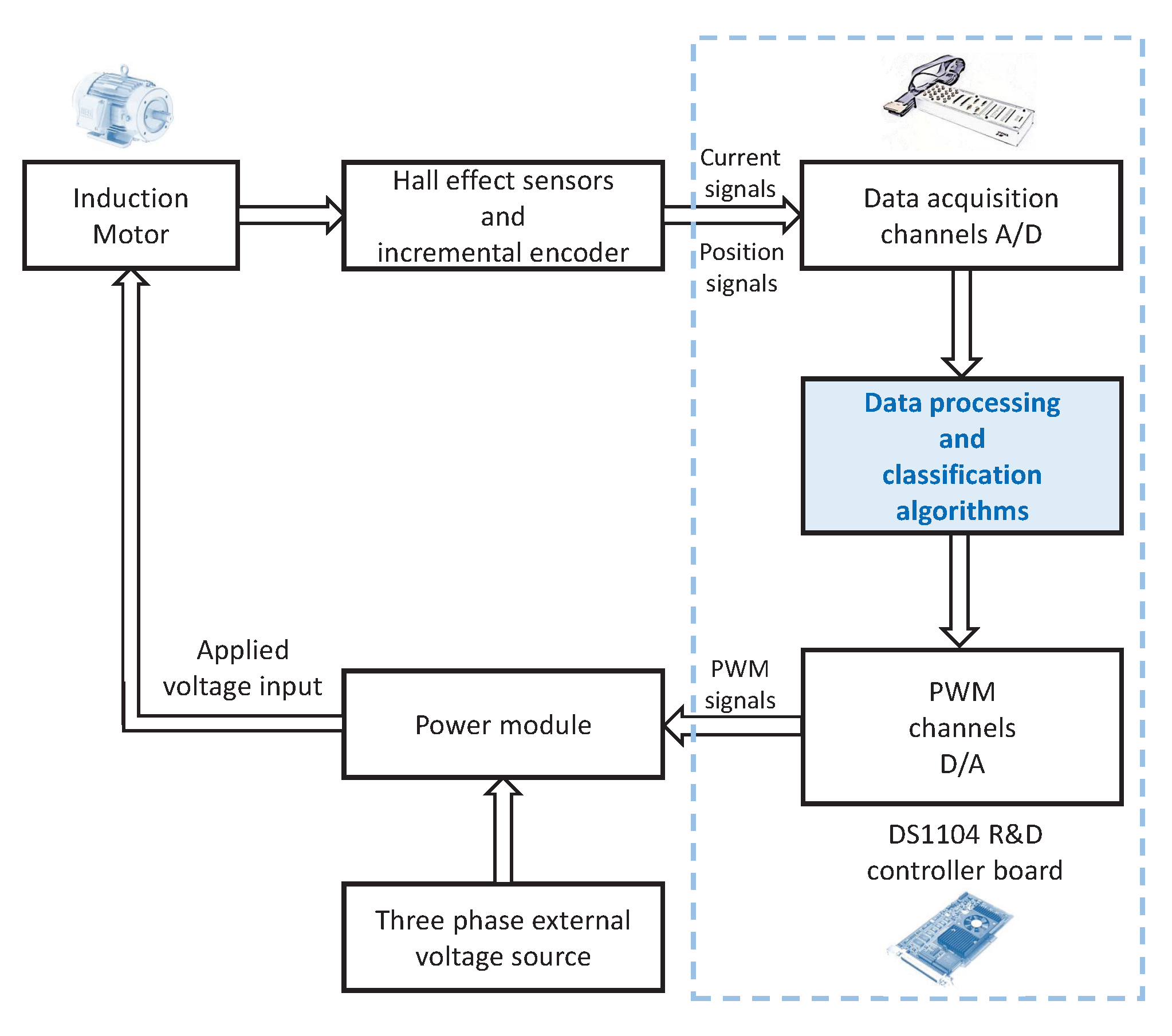
Figure 1. Rotatory induction motor test bench configuration for sensor fault classification.
Machines 10 01198 g001
Figure 2. Rotatory induction motor test bench for sensor fault classification.
Machines 10 01198 g002
Figure 3. Representative diagram of the structure of CNN for the classification of time series, where m is the number of classes.
Machines 10 01198 g003
Figure 4. Components of a fault-tolerant control that are prone to failure. u ( t ) is the control signal, u ¯ ( t ) the actuator signal, x ( t ) the system signal, x ¯ ( t ) the sensor signal and t the current sample.
Machines 10 01198 g004
Figure 5. The sliding-window embedding extracted of the time series, which serves as the input to neural networks.
Machines 10 01198 g005
Figure 6. Configuration of all neural networks used to classify faults of sensed data. I α ( t ) = [ i α ( t ( d 1 ) ) , , i α ( t ) ] and I β ( t ) = [ i β ( t ( d 1 ) ) , , i β ( t ) ] are delayed vectors.
Machines 10 01198 g006
Figure 7. Configuration of all neural networks used to classify faults of actuator data. U α ( t ) = [ u α ( t ( d 1 ) ) , , u α ( t ) ] and U β ( t ) = [ u β ( t ( d 1 ) ) , , u β ( t ) ] are delayed vectors.
Machines 10 01198 g007
Figure 8. Flowchart of the offline and online processes.
Machines 10 01198 g008
Figure 9. Sensor channel data set from the induction motor.
Machines 10 01198 g009
Figure 10. Actuator channel data set from the induction motor.
Machines 10 01198 g010
Figure 11. Comparison of failure classification.
Machines 10 01198 g011
Figure 12. Comparison for I α with different d values.
Machines 10 01198 g012
Figure 13. Comparison for I β with different d values.
Machines 10 01198 g013
Figure 14. ROC curve for u α .
Machines 10 01198 g014
Figure 15. ROC curve for u β .
Machines 10 01198 g015
Figure 16. Confusion matrix plot for Channel 3 with 10-d delayed vector. True positive: Neuronal classifier correctly predicted no failure. True negative: Neuronal classifier correctly predicted failure. False positive: Neuronal classifier incorrectly predicted no failure. False Negative: Neuronal classifier incorrectly predicted failure.
Machines 10 01198 g016
Figure 17. Confusion matrix plot for Channel 4 with 10-d delayed vector.
Machines 10 01198 g017
Figure 18. Confusion matrix plot for Channel 5 with 10-d delayed vector.
Machines 10 01198 g018
Table 1. Fault labels in sensors.
LabelFault
0Healthy
1None
2Position
3Current i α
4Current i β
5Position and current i α
6Position and current i β
7Current i α and current i β
8None
9Position, current i α and current i β
Table 2. Fault labels in actuator.
LabelFault
0Healthy
1Voltage u α
2Voltage u β
3Voltage u α and voltage u β
Table 4. Results obtained with all the proposed neural networks.
Neural NetworkMLPLSTMBiLSTMCNN
ChannelSensordAUCCAAUCCAAUCCAAUCCA
1Position211111111
2Current i α 80.97900.96650.98640.97780.98730.93810.98450.9665
100.97830.96660.97910.96750.97870.93180.99650.9909
3Current i β 80.98670.97410.99540.98920.99140.98230.98780.9731
100.98620.97180.99610.98960.99020.98210.99830.9942
4Voltage u α 80.98010.96780.99710.99050.99620.98870.99630.9807
100.97580.97590.99720.99070.99640.98900.99870.9957
5Voltage u β 80.98830.87370.99730.99110.99710.99070.99200.9753
100.98460.88230.99720.98450.99650.99090.99850.9930
Publisher’s Note: MDPI stays neutral with regard to jurisdictional claims in published maps and institutional affiliations.