Abstract
A high vacuum environment safeguards the performance of special processing technologies and high-precision parts such as nanosecond laser processing, chip packaging, and optical components. However, it poses higher requirements for the machine tool, which makes the temperature control of machine tools an important goal in design and development. In this paper, the thermal properties of a large-scale 5-axis laser processing machine tool in a vacuum environment were investigated. The thermal contact resistance between parts is identified by the parametric simulation and experiment. The whole machine temperature field was then obtained based on the fluid–thermal coupling model and verified by experiment. The results showed that the thermal contact resistance of the motor and reducer with the water cold plate was 560 W/(m2∙°C) and 510 W/(m2∙°C), respectively, and the maximum temperature increase of the machine was 3 °C. Based on the results, the machine tool’s temperature increase prediction chart was obtained by simulation under different processing conditions such as cooling water flow rate, cooling water temperature, motor speed, and ambient temperature. It provides technical and data references for the research on the thermal stability of the machine tool in processing.
1. Introduction
With the development of the manufacturing industry, vacuum environment processing is finding more and more applications. Not only do semiconductor devices, optical lenses [1], and other parts and equipment with special processing requirements need to be produced in a vacuum environment, but even the processing of ordinary parts is also turned to a vacuum environment processing [2] to improve surface roughness.
The vacuum environment poses higher thermal performance requirements for machine tools. It is well known that even in the atmospheric environment, the thermal error of machine tools accounts for more than 40% of all error sources [3]. The heat dissipation effect of air, especially the temperature-related parameters such as flow rate, temperature, outlet pressure, and heat-transfer coefficient, is the most important research areas in the research of machine tool performance [4]. In a vacuum environment, the air is so thin that it hardly exists, air convection cannot be formed, and processing equipment such as machine tools can only dissipate heat through heat radiation and heat conduction between components. This special thermal boundary condition raises higher requirements on the thermal characteristics of the machine tool during the working process. Therefore, it is urgent to conduct in-depth research on the thermal characteristics of machine tools in a vacuum environment so as to achieve accurate thermal performance by predicting and controlling the temperature increase of the whole machine.
When analyzing and predicting thermal characteristics of machine tools, the accuracy of input parameters is an important prerequisite for ensuring the correctness of thermal design results. The identification methods of input parameters for thermal characteristic analysis and prediction research in the field of machine tools can be roughly divided into theoretical analysis [5,6,7], experimental measurement [8,9,10,11,12,13,14,15,16,17], and numerical prediction [18,19,20,21]. For the references involved in the above three research methods, the application of different research methods is described in detail from the perspective of atmospheric and vacuum environment.
In an atmospheric environment, Laraq [5] is based on the linear superposition method to determine the heat-transfer coefficients of the contact surfaces of multiple discs of random location and size, providing an accurate analytical solution with a reasonable computation time. Meng et al. [6] believed that the influence of fractal parameters on the thermal and contact characteristics of the electro-spindle should not be ignored, so they established a mathematical model of the electro-spindle considering the influence of each fractal parameter, divided the key nodes of the electro-spindle, solved the heat balance equation, and finally the accuracy of the thermal resistance network model was verified by the temperature increase experiment. Mori et al. [8] studied the influence of the difference in the linear expansion coefficient between the machine tool and the workpiece on the thermal deformation caused by room temperature through precision machining experiments. Liu [9] proposed a method-combining experiment and prediction to analyze the temperature field of an EDM machine tool spindle. Zhang et al. [10] studied the contact thermal resistance of five aluminum alloy materials through experiments, and used the difference in average roughness produced by lathes with different feed speeds to characterize the surface topography of the contact surface. The results showed that there is no direct relationship between the contact thermal resistance and the surface roughness due to the different morphologies and contact randomness of the two surfaces during the contact process. Surface roughness and surface flatness have a coupled effect on the contact thermal resistance. Duo et al. [11] studied the effects of interface temperature, sample surface roughness, and contact pressure on thermal contact conductance through experiments. The results showed that the contact thermal resistance has a power–law relationship with the contact pressure and the interface temperature. Cheng et al. [18] carried out the finite element method simulation of thermal characteristics of a high-speed motorized spindle system under a high-temperature and high-pressure environment, and considered that the accurate determination of heat generation rate, convective heat-transfer coefficient, and heat-transfer coefficient is the basis for accurate simulation analysis of the thermal characteristics of the motorized spindle. Weng et al. [19] used the finite element method to match the thermal power-deformation mapping coefficient, and formed a general thermal-balance design method machine tools in an atmospheric environment based on the analytical modeling method. On the basis of the multi-point contact model, Liu et al. [20] considered the temperature dependence of the material, the thermal radiation through the cavity at the interface and the influence of the thermal interface material, and proposed a finite element model of high temperature thermal contact resistance. The geometric parameters of the finite element model were determined by simple surface roughness tests and experimental data fitting. The validity of the finite element model was verified by the experimental results of the high-temperature thermal contact resistance between the superalloy and the composite material.
For equipment in a vacuum environment, Chen et al. [7] proposed a data-processing technique for measuring contact thermal resistance. First, it was proved by numerical prediction that the thin disk sample is a one-dimensional axial heat flow, and an experimental device for measuring high-temperature thermal contact thermal resistance based on the steady-state method was established. The uncertainty of the method was less than 10%. Sun et al. [12] obtained the effects of interface temperature, contact pressure, surface roughness, heat flow, load cycle, and processing technology on the heat-transfer coefficient through experiments. Tian [13] mainly studied the water-cooled heat dissipation of the motor and the reducer, and determined the heat-transfer coefficient between the motor, the reducer, and the water-cooled plate through experiments. Chen [14] prepared samples with different surface roughnesses, and tested them in a vacuum environment and non-vacuum environment for thermal measurements, and proposed a surface roughness that can keep the contact thermal resistance consistent in various environments. Nishino et al. [15] simulated the actual heat-transfer surface of a cold-plate heat exchanger used in outer space with a square test plate made of aluminum alloy to study the thermal conductivity in a vacuum environment under low load. The microscopic and macroscopic thermal shrinkage resistances were evaluated based on the real contact pressure distribution and through digital image processing, and the results showed that the macroscopic shrinkage resistance caused by surface corrugation and substrate deformation had the greatest effect on the transformation of thermal conductivity at low applied loads. Ding et al. [16] established an experimental device to study the thermal conductivity of stainless-steel joints in vacuum, and analyzed the influence of the interface contact pressure and average interface temperature on the contact thermal conductivity. The results showed that the thermal conductivity reached the peak when the contact surface pressure was 25.54 MPa. Dongmei et al. [17] used the laser photothermal method to measure the contact thermal resistance between solids in the temperature range of 70~290 K and the pressure range of 0.2~0.7 MPa. The effects of temperature and contact pressure on the interface contact thermal resistance were analyzed. The relationship between contact thermal resistance and temperature under certain contact pressure is established. Li [21] determined the turntable structure scheme based on the finite element analysis method, optimized the main support structure with justified material selection, and analyzed and calculated the influence of the drive mechanisms and shafts on the turntable stiffness, temperature adaptability, and pointing accuracy.
These analysis studies show that the accurate identification of the heat-transfer coefficient between the contact surfaces is a key issue in the construction, analysis, and prediction of the thermal field model of the whole machine. There is still a lot of uncertainty in the theoretical calculation method of the heat-transfer coefficient. Due to the difference in contact pressure and surface roughness, there is no general formula for the contact surface; the experimental measurement method of the heat-transfer coefficient is relatively complicated, which is not suitable for large-scale machine tools. At present, there are relatively few studies on the thermal characteristics of equipment in a vacuum environment, and there is no research on the analysis, identification, and prediction of thermal characteristics of large-scale machine tools in vacuum.
Based on the heat flow coupling model, this paper identified the simulation parameters of a large machine tool in vacuum, affirmed that the key thermal characteristic parameter is the heat-transfer coefficient of the water-cooled plate in the motor-reducer system, and focused on its accurate identification. Through accurate thermal characteristic parameter identification, the consistency between theoretical simulation and experimental verification of the temperature field analysis of the whole machine in a vacuum environment was ensured. Therefore, the prediction research of the temperature field of the machine tool under various working conditions was carried out, which provides theoretical guidance for the performance analysis and thermal protection design of vacuum equipment.
2. Research Methodology
2.1. Analysis of Thermal Characteristics of Large Machine Tools in Vacuum
The research object of this project was a large five-axis machine tool that works 24 h in a vacuum environment. The X, Y, and Z moving axes travel a distance of 4 m × 4 m × 0.5 m. The three-dimensional model of the machine tool is shown in Figure 1a. The machine tool consists of three translational axes and two rotating axes. The components of the translational axis are as follows: servo motor-reducer, linear guide, screw nut, and bearing group; the components of the rotation axis are motor-reducer and bearing. The driving method of the translation shaft is that the rotating torque generated by the motor acts on the screw nut after passing through the reducer to drive the moving parts, and the rotating parts of the rotating shaft are directly connected to the reducer connected to the motor. During the machining process of the machine tool, the motor-reducer system will heat up severely. In order to control the temperature of the system and not affect the machining accuracy of the whole machine, a water-cooling plate was wrapped around the motor-reducer assembly, and cooling water was introduced to take away the heat generated by the motor and reducer, wherein the inner diameter of water-cooling plate runner was 10 mm. The heat, motor-reducer-water-cooling plate assembly is shown in Figure 1b.
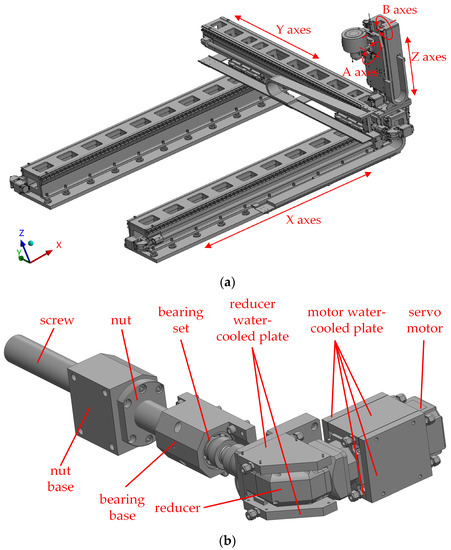
Figure 1.
3D model of the whole machine and the components of the translation shaft: (a) 3D model of the whole machine; (b) Components of the translation shaft.
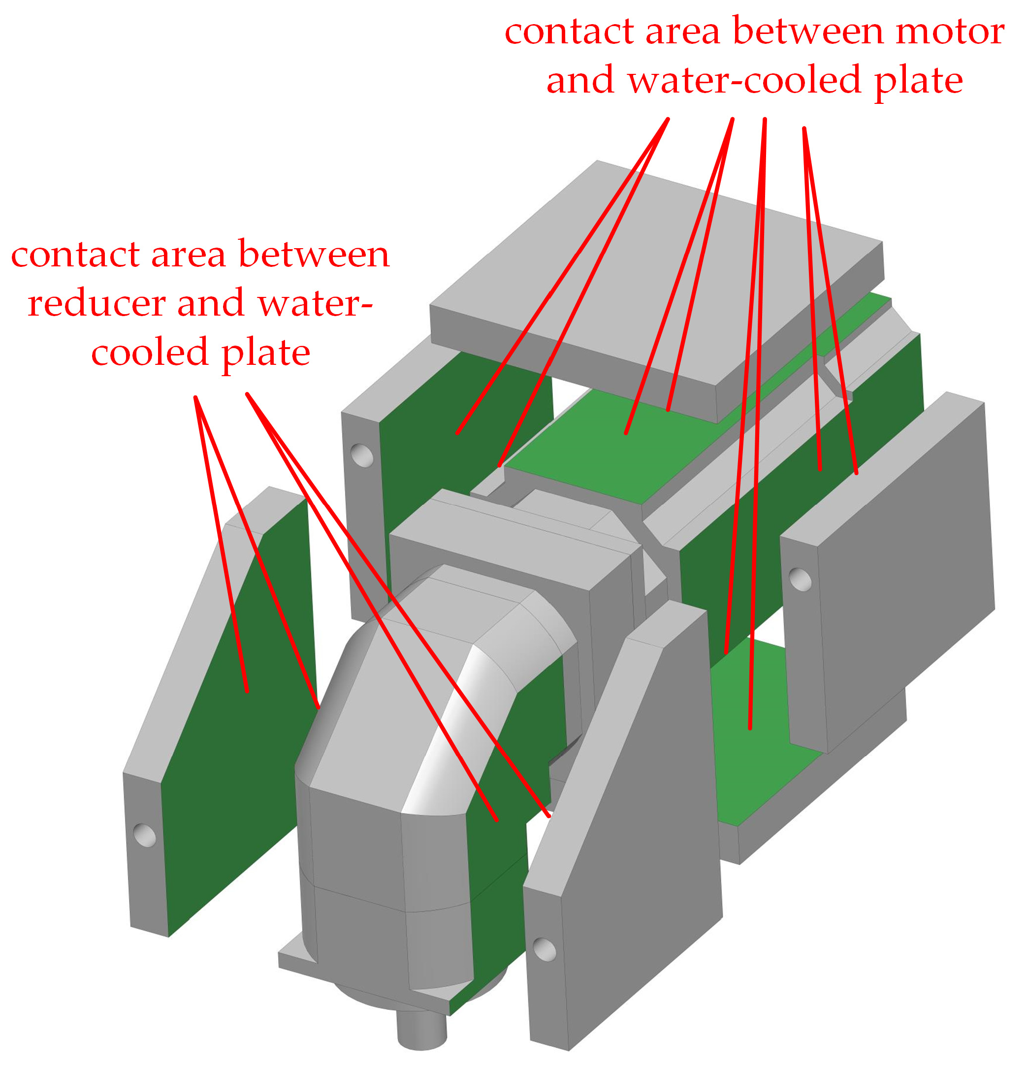
There are three ways to confirm the thermal characteristic parameter values: obtain the accurate value through formula calculation, such as the heating power of the motor and reducer; the empirical value, such as the external surface emissivity of the whole machine, and other thermal parameters that have little influence on the temperature field of the whole machine; finally there are also some parameters that are difficult to obtain through formulas and have no reliable empirical values, such as motors, reducers, and their respective water-cooling plates. Among all the parts of the whole machine, the motor and the reducer generate the most heat, so it is necessary to wrap the water-cooling plate around them and then feed the cooling water. The temperature difference between the two parts is the most disparate. The position of the contact surface of the motor, reducer, and its water-cooled plate is shown in Figure 2. The performance determines the accuracy of the simulation results. In this paper, after the key parameter identification and calibration of the heat-transfer coefficient between the motor reducer and its water-cooled plate was completed through experiment and simulation, in a vacuum environment, the simulation model of the whole machine was established, and the design and research process of the simulation and prediction of the thermal characteristics of the whole machine was carried out.
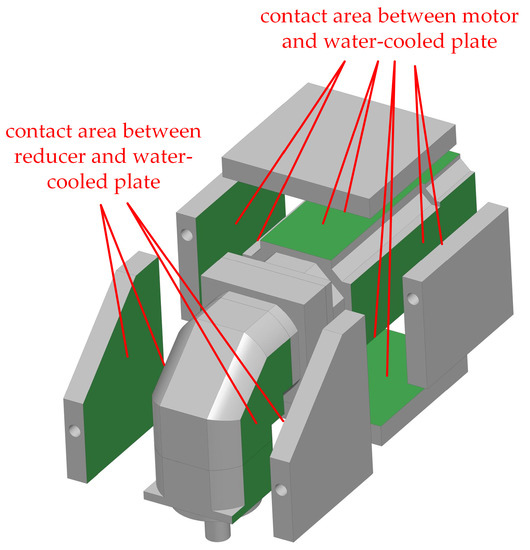
Figure 2.
Heat-exchange contact surface.
The temperature increase of the whole machine is large in the vacuum environment. In order to reduce the error caused by the thermal deformation of the parts during the temperature increase of the parts, the machine tool is preheated before processing. It can be considered that the machine tool works in a stable state of the temperature field of the whole machine, so a unidirectional steady-state flow-thermal coupling simulation model was established for analysis. The simulation process is shown in Figure 3. The steady-state flow field and steady-state thermal analysis module were established using ANSYS Workbench. First, the surface temperature of the cold-plate runner under the action of cooling water was obtained through the Fluent module, and then the temperature was imported into the steady-state thermal module to calculate the temperature field of the whole machine. The main boundary conditions imposed by the flow field were as follows: cooling water temperature, flow velocity, etc., and the main boundary conditions imposed by the thermal field were as follows: heat flux density, ambient temperature, vacuum emissivity, etc.
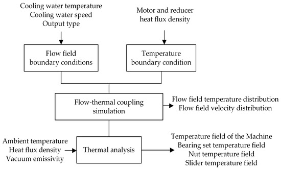
Figure 3.
Simulation flow chart.
2.2. Heat Source Calculation
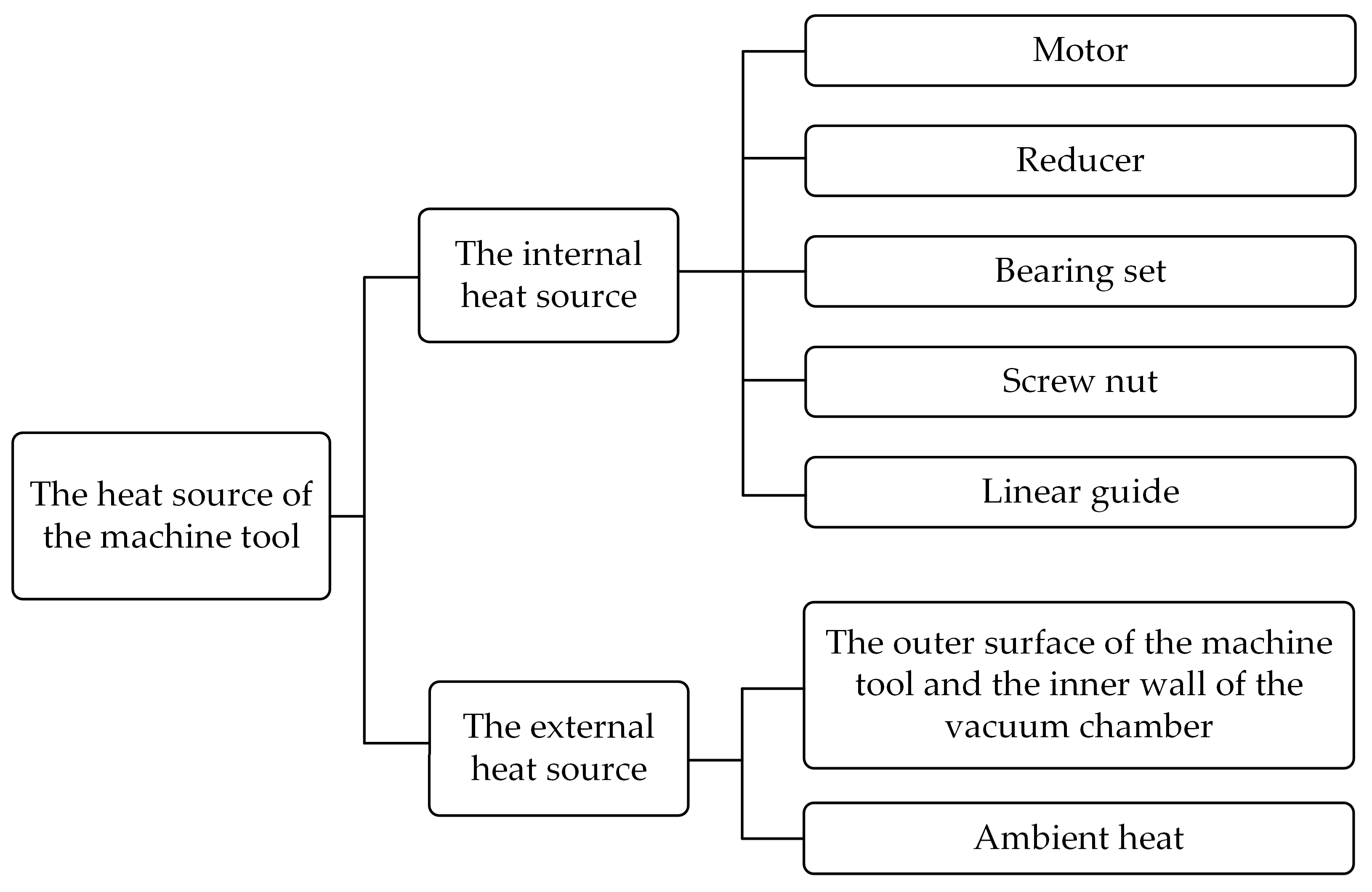
The heat source of the machine tool in the working process has two parts, as shown in Figure 4: one is the internal heat source in the feeding system, mainly the heat generated by the rotation of the motor reducer and the friction heat generated by the motion pair between some parts; the other is the external heat source acting on the machine tool, which is mainly the radiation heat exchange between the ambient heat and the outer surface of the machine tool and the inner wall of the vacuum chamber. The heating power value of the internal heat source can be obtained through a calculation method; for the external heat source, the ambient temperature can be obtained through a temperature sensor.

Figure 4.
Heat source diagram of the whole machine.
According to the specific component assembly and load of the machine tool studied in this paper, with reference to relevant literature [22,23] and empirical formulas, the total load inertia converted from the components on the motion axis to the motor was first calculated, including Jscrew, Jcoupling and JL; the heating power of the internal heat source was calculated, including the feed acceleration torque Ma of the motor shaft, the additional friction torque Mscrew friction of the lead screw preload, the additional torque of the guide rail friction Mrail friction, and bearing friction additional torque Mbearing friction. The four types of torques are given below, and the starting torque Ms of the motor can be calculated accordingly, as shown in Formulas (1)–(5).
where Jload—the total load inertia of the screw, coupling, reducer, etc. converted to the motor shaft, unit: kg·m2;
- JR—reducer inertia, the specific value can be obtained from the sample unit: kg·m2;
- Jscrew—the inertia of the lead screw converted to the motor shaft, unit: kg·m2;
- m2—mass of ball screw, unit: kg;
- D2—ball screw diameter, unit: m;
- i—reduction ratio, it can be seen from the sample that its value is 5;
- Jcoupling—the moment of inertia converted from the coupling to the motor shaft, unit: kg·m2;
- m3—coupling mass, unit: kg;
- D3—coupling diameter, unit: m;
- JL—the inertia of the moving parts converted to the motor shaft, unit: kg·m2;
- P—screw lead, unit: m.
- n—motor speed, unit: r/min;
- T—The theoretical acceleration time of the motor is 0.2 s according to the design experience;
- FP—preload force, unit: N;
- L—lead of the screw, unit: m;
- ηR—reducer efficiency is 0.95 according to the technical manual;
- η0—the efficiency when the lead screw is not preloaded is 0.95 according to the technical manual;
- μ1—the friction coefficient of the guide rail is 0.01, according to the design experience;
- m—the weight of the moving parts, unit: kg;
- μ2—bearing friction coefficient is 0.0025 according to the technical manual;
- P—bearing load, unit: N;
- d—the inner diameter of the bearing, unit: m.
Through the above torque and motor speed and the efficiency of the motor reducer, the heating power Qmotor and Qreducer of the motor and the reducer can be calculated. The heating power of the bearing and the lead screw Qbearing friction and Qscrew friction can be calculated according to the corresponding torque and speed, and the heating power Qrail friction of the guide rail depends on the friction coefficient between the guide rail sliders, the axle weight, and the moving speed. The specific calculation formula is shown in Formula (5).
where, ηM—motor efficiency is 0.9, according to the technical manual, the value
- v—movement speed of moving parts, unit: m/s.
According to the design requirements, the maximum moving speed of each axis is 100 mm/s, and the maximum speed of the motor is 2500 r/min; substituting the practical parameters such as screw lead and the weight of the moving parts into the equation, the heating power of each heating source can be calculated as shown in Table 1.

Table 1.
Heating power.
In the machining process, the Y axis is the main motion axis, and the parameter-identification method and process of the whole machine are explained by taking the parameter identification of each component of the feed system on the Y axis as an example. After substituting the relevant parameters of the Y-axis, it can be calculated that the total inertia of the load converted to the motor by the Y-axis motion system is 4 N·m, and the heating power of the components of the feed system is shown in Table 2.

Table 2.
The heating power of each component of the Y-axis motor at different speeds.
2.3. Simulation Model of Motor-Reducer System
Before the simulation analysis of the motor-reducer system, the detailed features and structural components such as holes, grooves, and chamfers in the model shall be simplified or deleted. The simplified model shall be imported into the ANSYS software and then divided into elements. The total number of nodes is 210,000. The specific simulation process of the system is as follows: (1) After assigning the temperature and flow rate at the cooling water inlet and the heat flux density on the heating surface of the motor and reducer in the Fluent module, the temperature distribution on the surface of the flow channel on the water-cooling plate is calculated. (2) Import the flow channel temperature obtained in the above steps into the steady-state thermal module of Workbench. (3) The main boundary conditions of the thermal module are as follows: the heat flow of the heating surface of the motor and reducer, the radiation rate of all external surfaces, and the temperature of the imported flow channel. The main material of the whole machine is stainless steel. In order to determine its surface emissivity, we first drive the Y-axis to reciprocate in a vacuum environment for several hours, record the temperature of each component at this time, then let the whole machine stand in a vacuum environment for 17 h, record the temperature of the corresponding parts again, and the temperature difference between the two bearing seats on the motor side is less than 2 °C. Since the temperature drop of the whole machine in a vacuum environment is mainly due to the thermal radiation of the surface, the initial boundary condition was set in the simulation software as the temperature before the whole machine rests, and the radiation rate was adjusted through parametric simulation to make the simulation results consistent with those after shutdown. The temperature of each part is the same, and the emissivity was obtained as 0.55. The main parameters applied to the simulation model in the vacuum environment are shown in Table 3. The main parameters applied to the simulation model in the vacuum environment are shown in Table 3.

Table 3.
Simulation parameters of the motor-reducer system.
The whole machine was simplified and imported into ANSYS for mesh generation, as shown in Figure 5. The total number of nodes is 4.97 million. The water-cooled plate is made of aluminum alloy, and the whole machine is made of stainless steel.
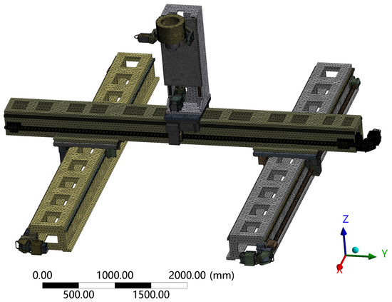
Figure 5.
Mesh diagram of the whole machine.
The main parameters imposed on the simulation model in the vacuum environment are shown in Table 4. The temperature of the water-cooling plate was imported from the simulation results of the motor-reducer system, and the heat-transfer coefficient of the motor system was subsequently identified and then assigned to the simulation model.

Table 4.
Simulation parameters of the whole machine.
After obtaining the heat source of the motor and reducer through calculation, the temperature of the water-cooled plate is expected to rise by 2 °C, the temperature difference between the inlet and outlet cooling water is expected to be 1 °C, and the average water temperature will rise by 0.5 °C. The expected average temperature difference of the cooling water is 1.5 °C. Substituting these data into the formula, it can be concluded that the cooling water flow rate is 3.957 × 10⁻⁵ m3/s.
where, q—cooling water flow, unit: m3/s;
- P—total heating power of motor and reducer, unit: W;
- c—specific heat capacity of cooling water, which is 4.2 × 10³ J/(kg·°C)
- ρ—cooling water density, which is 1.0 × 10³ kg/m3
- ΔT—temperature difference between water outlet and water inlet, unit: °C.
3. Identification of Key Parameters Based on Experiments
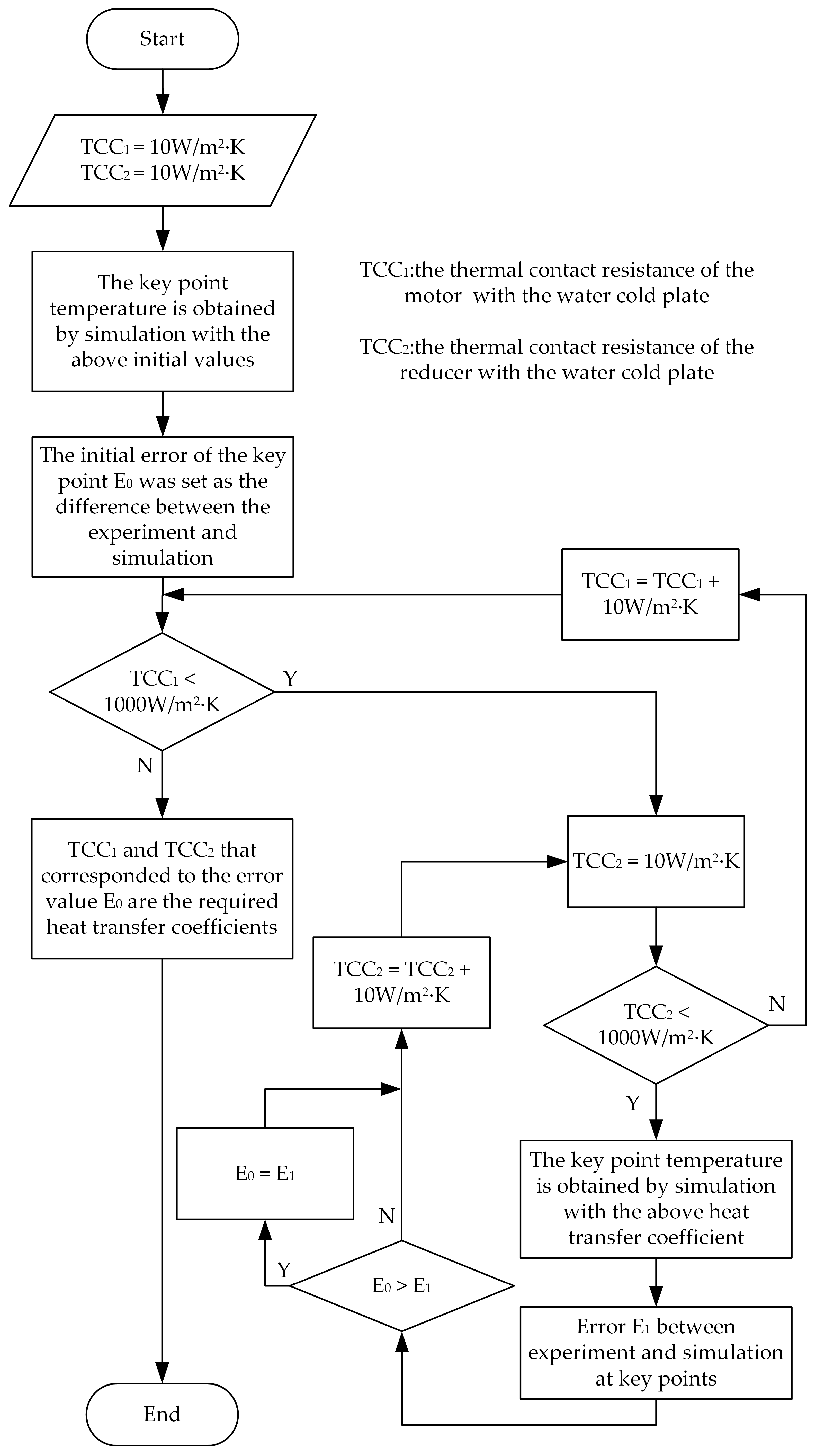
In the thermal characteristic model, the contact pressure and surface roughness between the contact surfaces of the motor, reducer and water-cooled plate are different, and the value of the heat-transfer coefficient between the two cannot be directly deduced and calculated through the theoretical formula, and the test measurement is difficult to achieve for the system, so it is a key parameter that is difficult to determine. In combination with test and simulation, this paper proposed a process to determine the heat-transfer coefficient. The basic steps are as follows:
- (1)
- Build a test platform to analyze the temperature increase of key parts such as the motor, reducer, and water-cooled plate surface under certain working condition (working condition 1);
- (2)
- Using the parametric simulation module of the finite element software, the heat-transfer coefficient value is obtained by cross-checking and verifying with the above test results. The specific process is shown in Figure 6.
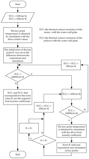 Figure 6. Flow chart of preliminary determination of heat-transfer coefficient.
 - (3)
- According to the thermal resistance value obtained in step 2, the temperature of the key position of the motor system under another working condition (working condition 2) is obtained through simulation;
- (4)
- Finally, verify the accuracy of the temperature through experiments.
3.1. Setting Up the Test Environment
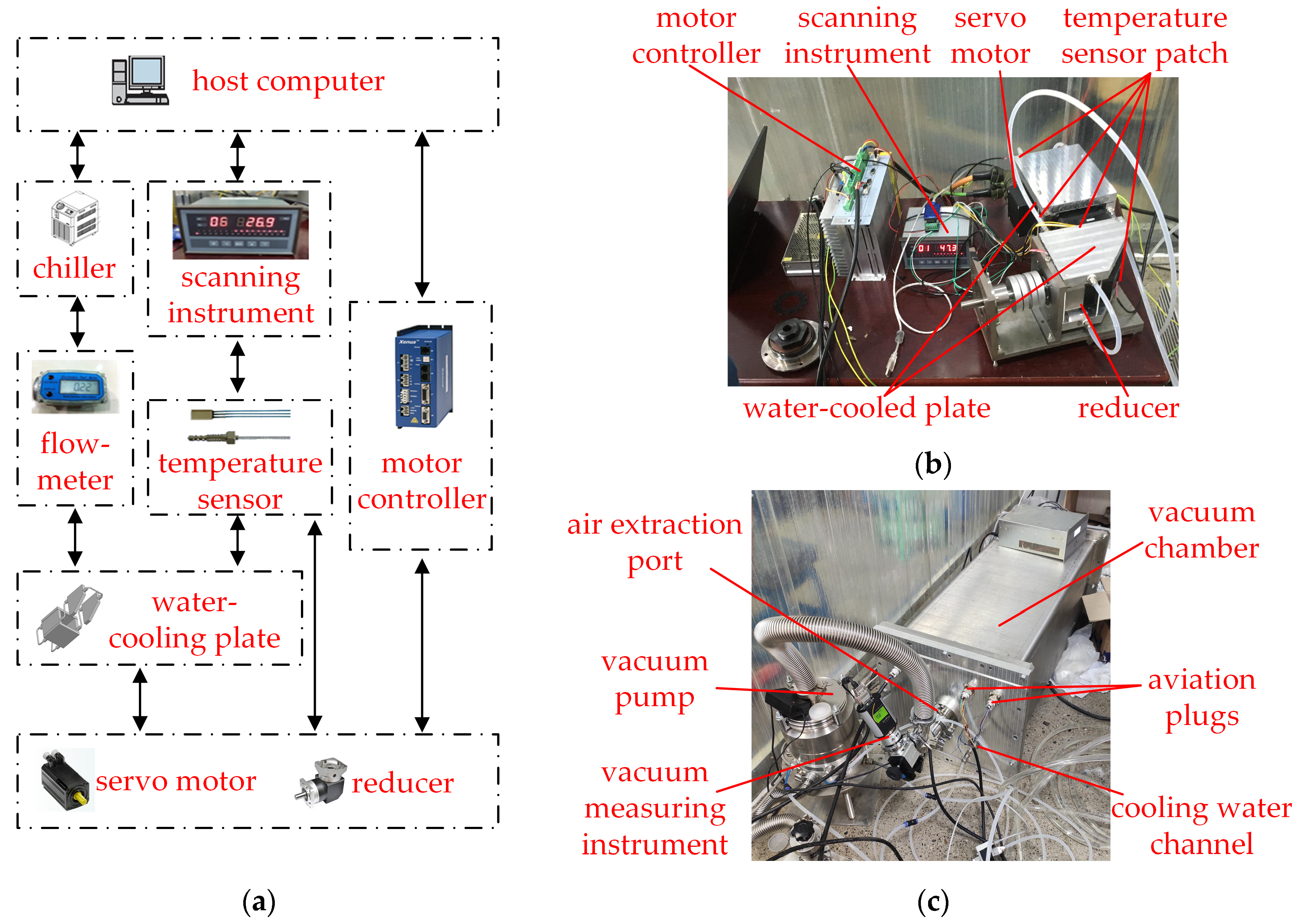
The test equipment and its connection method are shown in Figure 7a; the host computer is connected to each equipment through RS232 cable, the water cooler and flowmeter monitor the operation status of each equipment during the test; the motor driver controls the parameters of the motor speed; the temperature of the motor-reducer system is obtained with the temperature sensor, and the important parameters of the test equipment are shown in Table 5.

Figure 7.
Motor-reducer system test platform: (a) Assembly schematic; (b) Parts Wiring Diagram; (c) Vacuum Chamber Wiring Diagram.

Table 5.
Equipment parameter table.
The assembly diagram of the external environment of the test platform is shown in Figure 7b. The motor-reducer system was connected to the water-cooling plate through bolts and studs, feeding cooling water into the water-cooling plate. The test platform was connected to the following three types of cables: (1) Communication cables. The host computer was connected to the motor controller through the RS232 communication line to adjust the parameters such as the motor speed, and the servo motor and the motor controller were connected through the feedback line; (2) The power line. The servo motor was connected to the 380 V power supply through the power line; (3) The temperature-sensor connection line. The inspection instrument obtained the temperature of key positions through temperature sensors attached to the motor, reducer, and water-cooling plate. After the test platform was assembled and tested in the atmospheric environment to ensure normal movement, the abovementioned connecting lines were connected to the power supply, the host computer, and the inspection instrument, respectively, through the two aviation plugs reserved in the vacuum chamber. In addition to the cable wiring, the cooling water channel and the air extraction port were also connected to the water cooler and the air-extraction machine through the interface reserved in the vacuum chamber. The connection of the vacuum chamber is shown in Figure 7c. In order to provide load for normal operation of the machine tool, the motor-reducer system test device uses friction torque limiter to provide load for the motor reducer. By adjusting the friction force of the torque limiter, the load change of the machine tool under actual working conditions was simulated. According to the motor output torque read from the servo motor feedback data, the pre-tightening nut of the torque limiter was adjusted until the output torque was equal to the driving torque design index of the large motion platform.
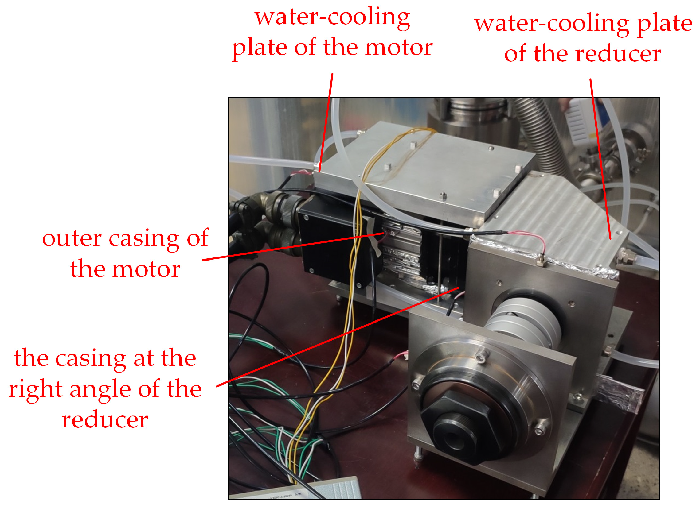
During the construction of the test platform, the location of the temperature sensor directly affects whether the test results are accurate and sound. As the two heat sources of the test platform, the motor and the reducer have a high overall temperature. It is necessary to arrange a sensor at the outer casing of the motor and the casing at the right angle of the reducer to monitor their temperature. The temperature of the water-cooling plate is greatly affected by the cooling water. A sensor was arranged on each of the two water-cooling plates. The sensor on the water-cooling plate of the motor was located at the cooling water inlet, and the sensor on the water-cooling plate of the reducer was located in the middle of the entire flow channel. Its value can be used as the average temperature of the water-cooling plate. The housing of the motor and reducer used a chip sensor to collect the housing temperature, and the water-cooling plate adopted a spring-loaded sensor, which can measure the internal temperature of the water-cooling plate. The placement of the sensor is shown in Figure 8.
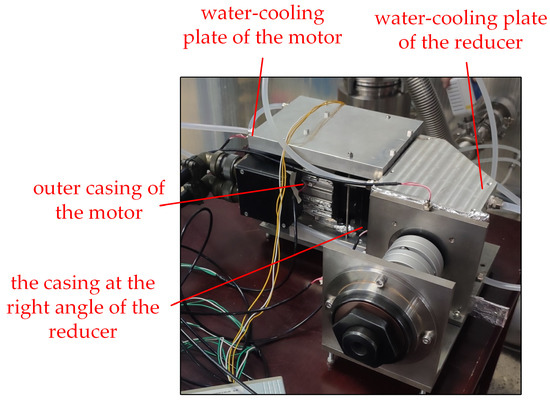
Figure 8.
Sensor placement position of the test platform.
3.2. Preliminary Determination of Heat-Transfer Coefficient
In order to obtain the heat-transfer coefficient accurately, two sets of test conditions need to be selected in combination with the motor performance and the actual processing conditions. For the motor speed part, the designed maximum speed is 2500 r/min, and the average speed when the equipment is in use is 1250 r/min; the cooling water temperature was uniformly set to room temperature. According to the test, when the cooling water flow rate is 3.33 × 10⁻⁵ m3/s, the design requirements are met, and when the flow rate is greater than 6.67 × 10⁻⁵ m3/s, the system has no further cooling effect. In summary, in the selected working condition 1, the motor speed is 2500 r/min, the cooling water temperature is 26 °C, and the flow rate is 3.33 × 10⁻⁵ m3/s; in working condition 2, the motor speed is 1250 r/min, the cooling water temperature is 26 °C, and the flow rate is 6.67 × 10⁻⁵ m3/s. The specific parameters are shown in Table 6.

Table 6.
Comparison table of working condition parameters.
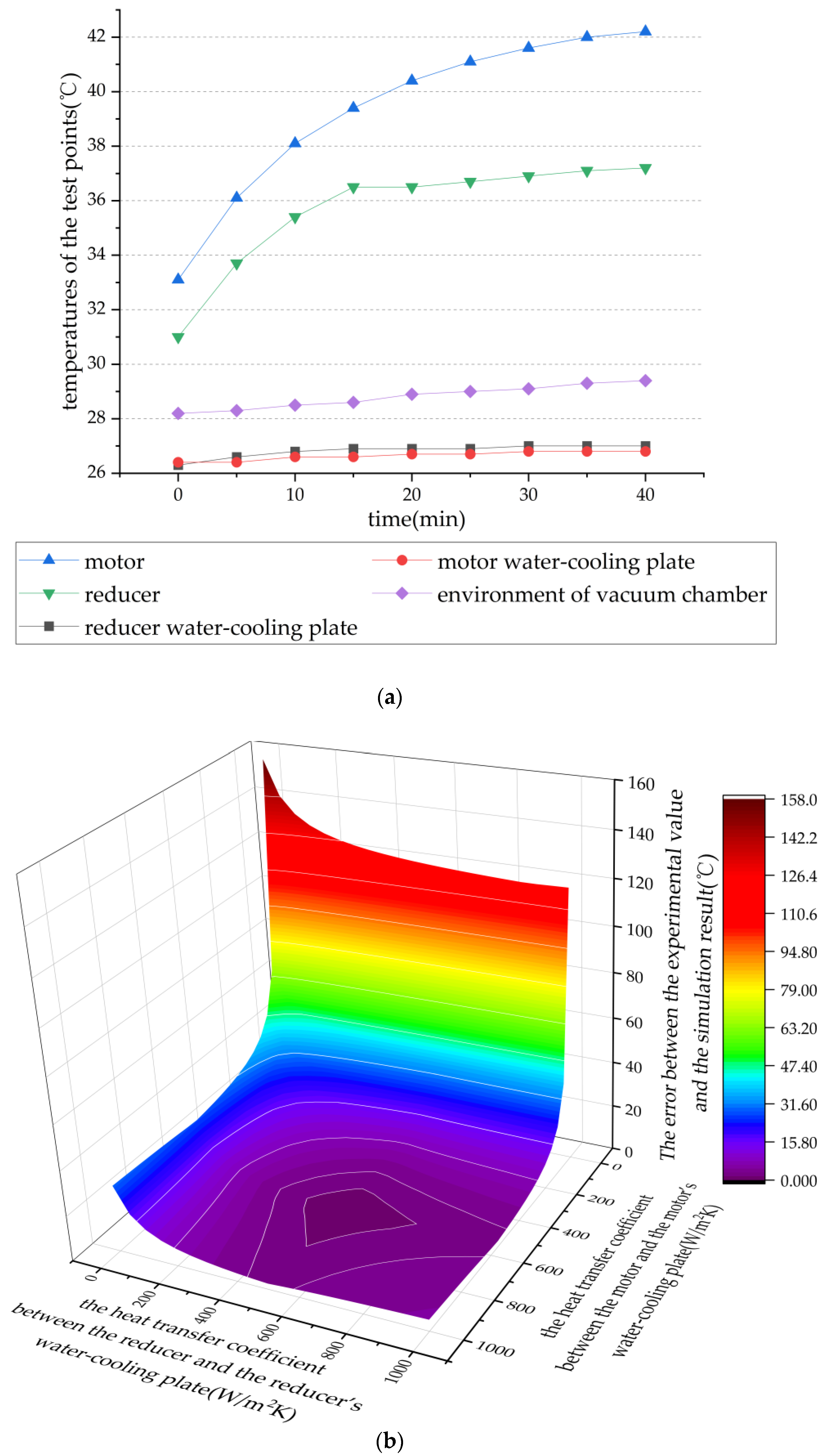
A pre-test was conducted to measure the temperature increase of the motor-reducer system. During the test, the average temperature of the vacuum chamber was 28.8 °C, and the temperature increase test of the motor-reducer system was carried out under the condition of working condition 1. The temperature of the sensor was recorded every 5 min, and the actual temperature increase is shown in Figure 9a. When the system ran for about 40 min, the temperature of the system tended to be stable. At this time, the temperature of the motor shell was 42.2 °C, the temperature of the reducer shell was 37.2 °C, and the temperature of the water-cooling plate was 26.2 °C and 26.5 °C.

Figure 9.
The test and simulation results of working condition 1: (a) Test temperature increase diagram; (b) The parameterized simulation results of working condition 1.
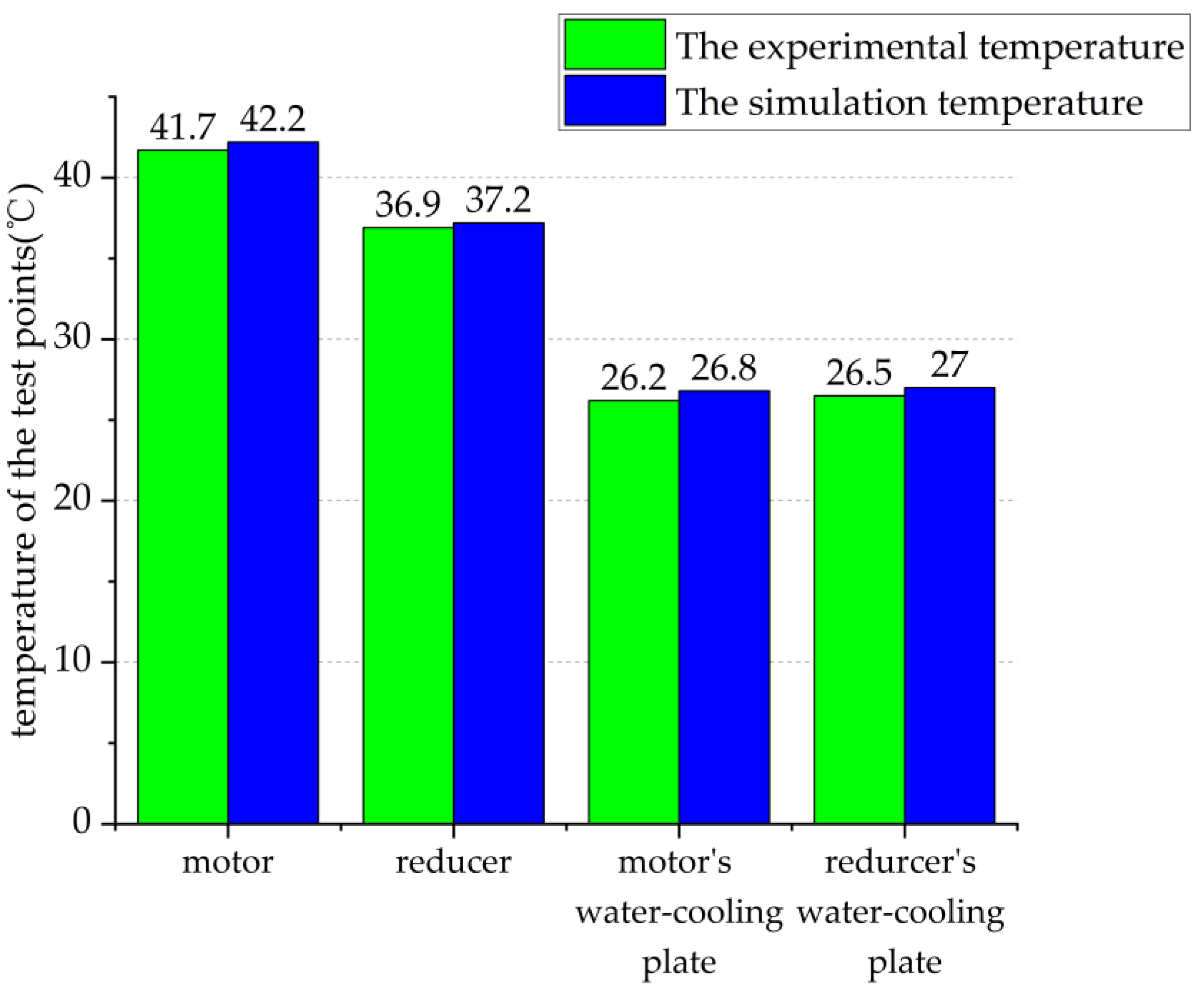
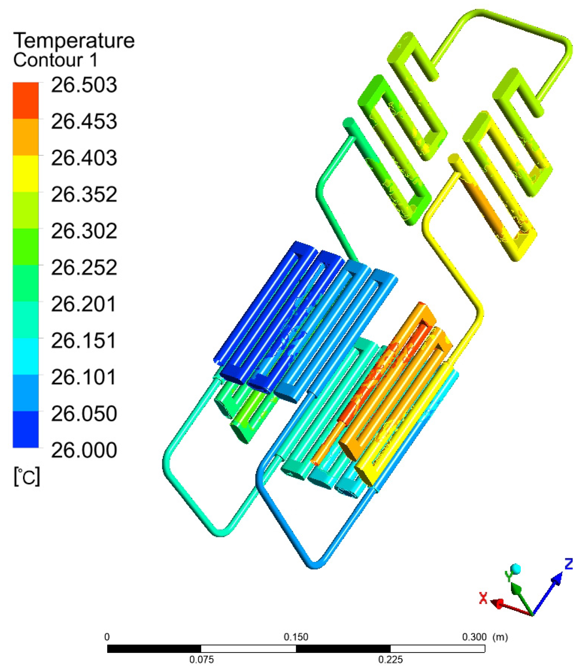
The heat-transfer coefficient between the contact surfaces was then obtained by parametric simulation in the simulation software. The simulation input parameters were set to be the same as the abovementioned test conditions. The parameterized simulation input parameters were as follows: the heat-transfer coefficient between the motor, the reducer, and their respective water-cooling plates, and the value range was 0~1000 W/(m2∙°C). The value interval was 10 W/(m2∙°C); the output parameter was the temperature of the component, and the specific position in the 3D model corresponds to the temperature sensor location. The simulation results are shown in Figure 9b, when the heat-transfer coefficient between the motor and the motor’s water-cooling plate was 560 W/(m2∙°C), and the heat-transfer coefficient between the reducer and the reducer’s water-cooling plate was 510 W/(m2∙°C); the error between the simulation results and the test temperature was the lowest. At this time, the motor temperature was close to 41.8 °C, the reducer housing was 37 °C, and the water-cooling plate temperatures were 26.2 °C and 26.5 °C, respectively. Comparing the simulation results with the temperatures obtained from the test, as shown in Figure 10, the maximum temperature difference between the two was 0.5 °C at the motor housing, 0.3 °C at the reducer housing, and 0.4 °C and 0.5 °C for the water-cooling plate. It is considered that the simulation result was close to the test temperature. Figure 11 shows the simulation result of cooling water temperature of working condition 1. The temperature at the inlet and outlet were 26 °C and 26.5 °C, respectively, and the difference between the two was 0.5 °C. In order to further verify whether the value is the real heat-transfer coefficient value, another set of working conditions (working condition 2) needs to be selected for simulation and experiment.

Figure 10.
Comparison of the simulated temperature in working condition 1 test.

Figure 11.
Simulation results of the cooling water temperature of working condition 1.
3.3. Verification of Heat-Transfer Coefficient
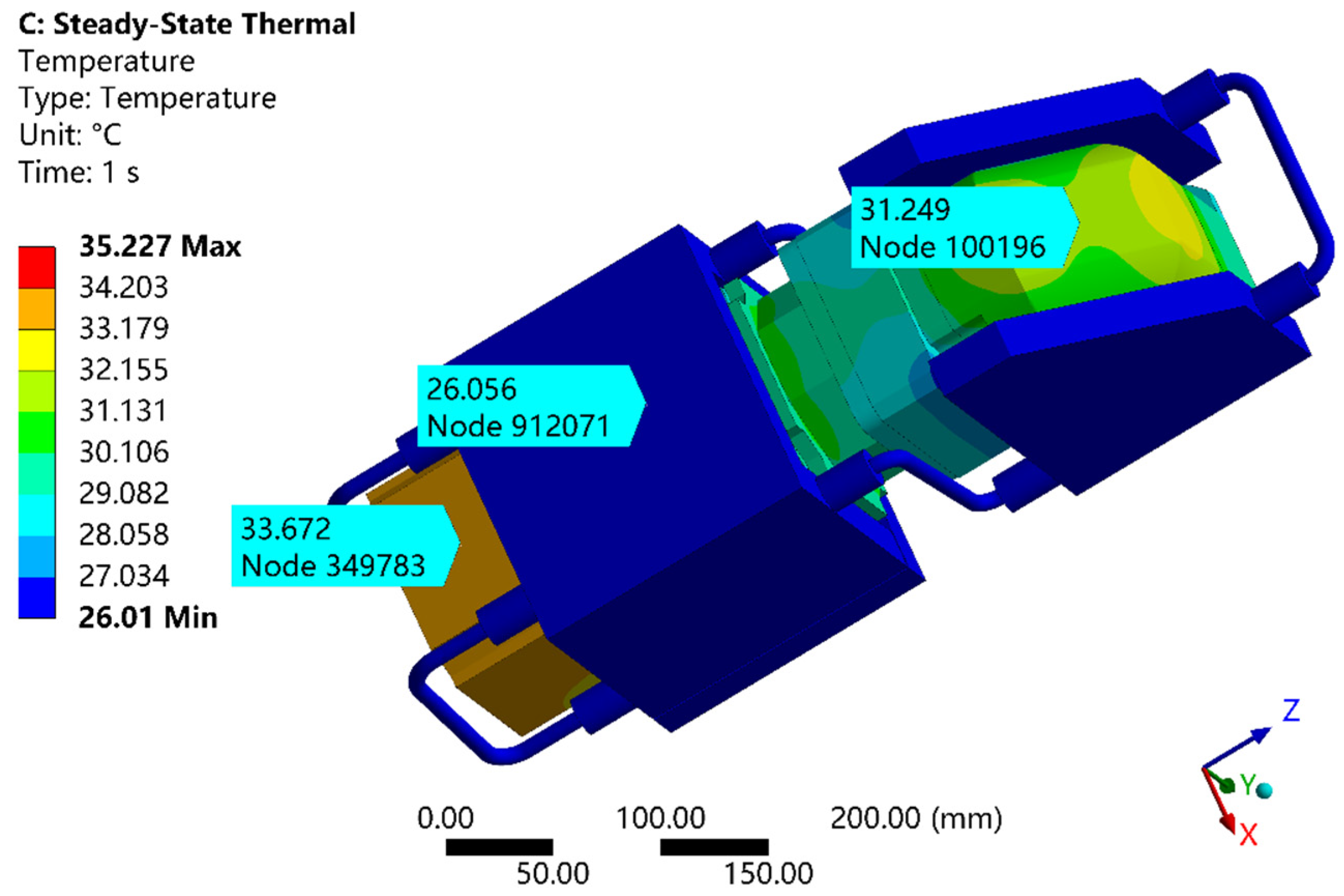
Under working condition 2, the abovementioned thermal resistance value was used for simulation. The results are shown in Figure 12. Under this working condition, the motor temperature dropped to 33.7 °C, the reducer housing was 31.2 °C, and the temperature increase of the water-cooling plate was stable at about 26.1 °C.
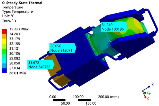
Figure 12.
Simulation results of working condition 2.
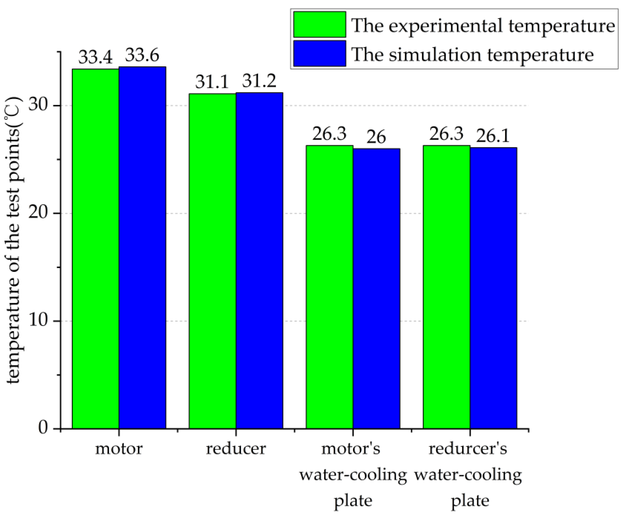
In order to verify the accuracy of the abovementioned simulation results, the same working conditions were used for the verification test and the sensor temperature was recorded every 5 min. After about 25 min, the system temperature tended to be stable. At this time, the temperature of the motor casing was 33.4 °C, the casing temperature of the reducer was 31.1 °C, and the water-cooled plate 26.3 °C. The simulation results were compared with the temperature obtained by the test. As shown in Figure 13, the temperature difference between the two at the motor water-cooling plate reached a maximum value of 0.3 °C, the temperature difference between the motor casing and the reducer water-cooling plate was 0.2 °C, and the reducer casing temperature difference was 0.1 °C.

Figure 13.
Comparison of simulated temperature in working condition 2 test.
In this section, two sets of tests and simulations were carried out for the motor-reducer system and a comparative analysis is carried out. Under the same working conditions, the temperature difference between the two does not exceed 0.5 °C, and the heat exchange between the motor reducer and its water-cooling plate is found. The coefficient values are 560 W/(m2∙°C) and 510 W/(m2∙°C).
4. Simulation Analysis and Verification of Thermal Characteristics of the Whole Machine
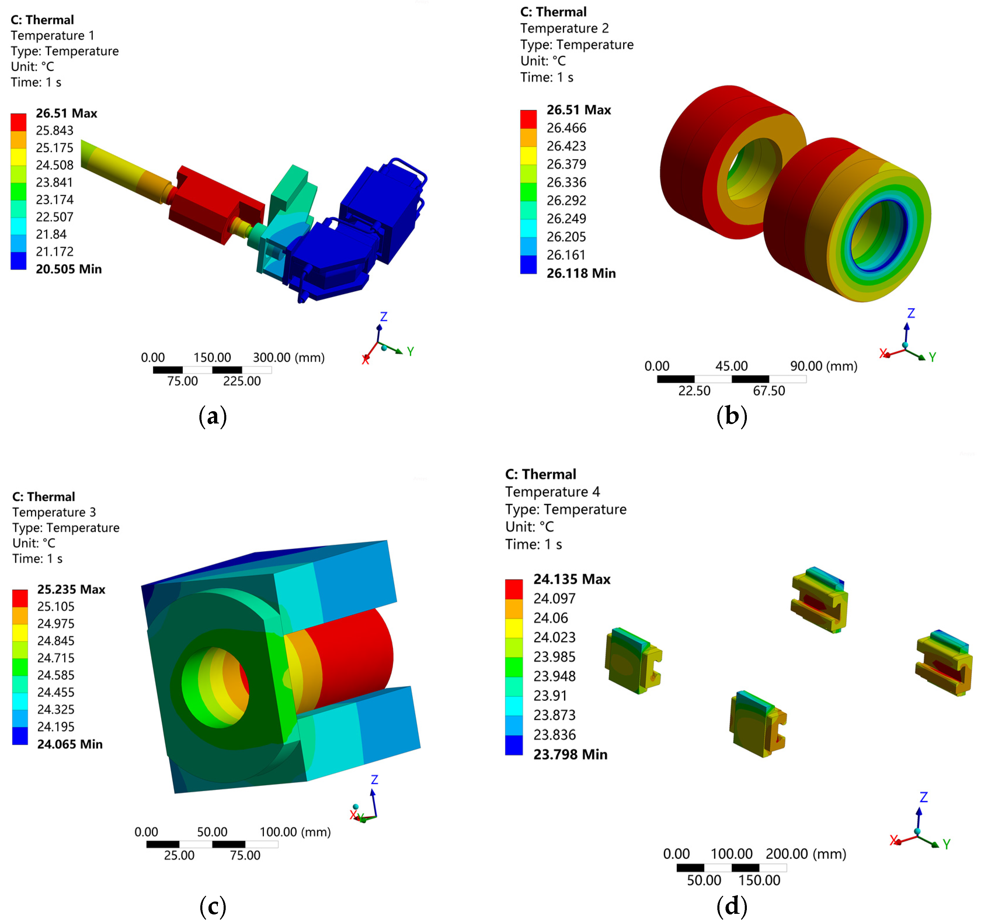
The identified contact thermal resistance was introduced into the whole machine simulation model, and the temperature distribution of the whole machine temperature field and the temperature of key points on the Y-axis could be obtained by combining other boundary condition values listed in Table 4, as shown in Figure 14. Figure 15 shows the temperature field distribution of key components on the Y-axis. The maximum temperature increase of the whole machine reached 3 °C, which appeared on the bearing on the motor side. Since the motor water-cooling plate passes through the cooling water of 20.5 °C, the overall temperature was not much different from the cooling water, which was within 0.1 °C. The temperature field analysis of some key components is as follows: (1) Different from the atmospheric environment, the temperature of the motor-reducer system was about 20.5 °C under the cooling effect of the cooling water, and the temperature of the motor base and the coupling was within 24.3 °C~20.5 °C; the temperature difference was large and there was an obvious gradient change; (2) the maximum temperature increase of the nut on the motor side was 3 °C, and the closer it is to the motor system, the lower the temperature; (3) the maximum temperature increase of the nut was 1.7 °C; (4) the maximum temperature increase of the slider was within 0.6 °C, and the minimum temperature increase was 0.3 °C. According to the simulation results, it can be considered that sensors should be installed at the following parts to monitor the temperature of the whole machine: (1) the highest temperature point of the machine tool is the motor side bearing, so a sensor should be attached to the bearing seat; (2) the temperature of the nut and slider also increased to a certain extent, so it is necessary to attach a temperature sensor to the nut bracket and the side of the slider; (3) as the main heat source, the motor and reducer should be attached with a sensor on the shell to ensure that the temperature is within the applicable range when the water-cooling plate is cooled; (4) a temperature sensor should be attached at the inlet of the water-cooling plate to monitor the temperature of the cooling water. It can be seen from the above analysis that the temperature measurement points of key components of the feed system should be as shown in Figure 16.
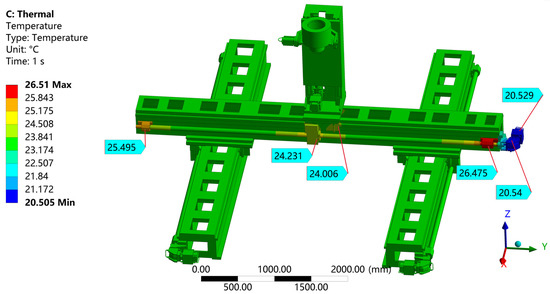
Figure 14.
Temperature field of the whole machine in a vacuum environment.
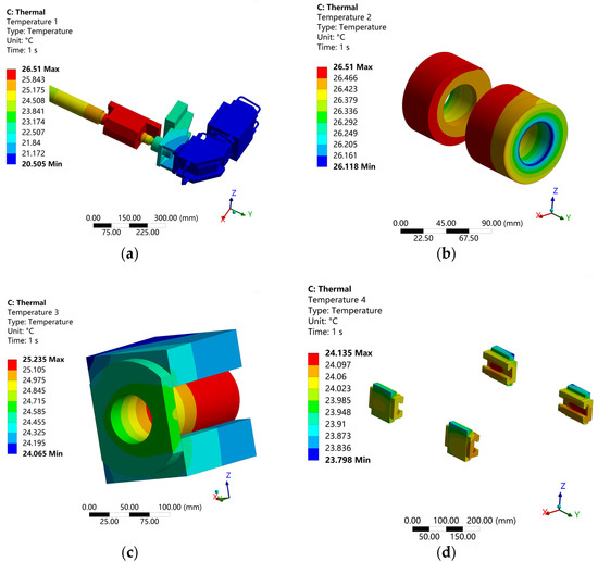
Figure 15.
Temperature of the key components in a vacuum environment: (a) Motor side temperature rise diagram; (b) Bearing set temperature rise diagram; (c) Nut temperature rise diagram; (d) Slider temperature rise diagram.
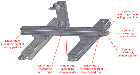
Figure 16.
Positioning diagram of the temperature sensor of the Y-axis feeding system.
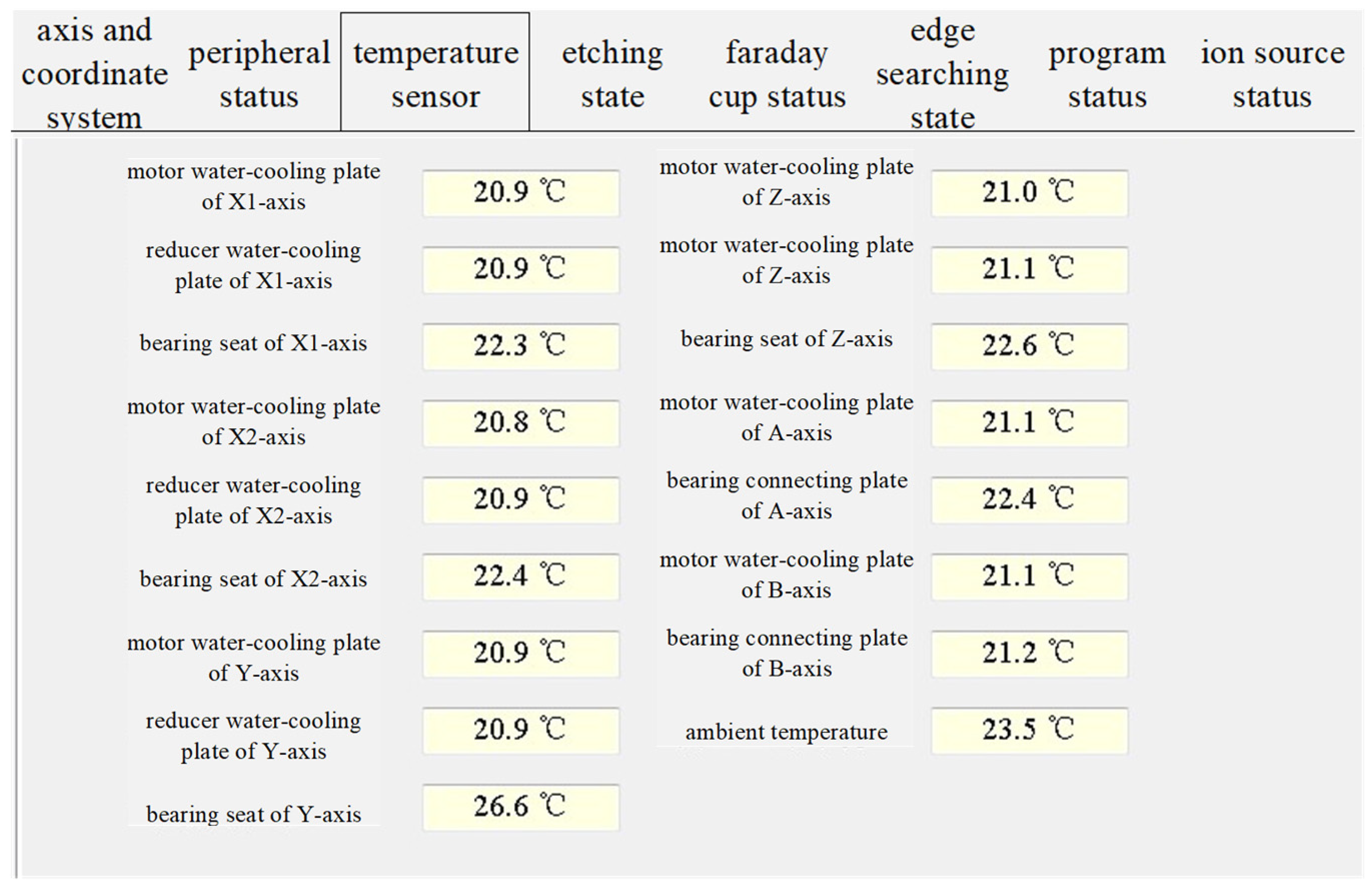
The test was carried out under the same simulation boundary conditions as given in Table 4; the Y-axis reciprocated at a speed of 10 mm/s, while the other axes remained stationary, and the Y-axis water-cooling plate was fed with cooling water of 20.5 °C. The temperature of the key components measured by the temperature sensor displayed on the host computer during the whole machine test is shown in Figure 17.
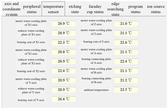
Figure 17.
Upper computer interface during the whole machine test.
The analysis of the three temperature sensors on the Y-axis showed that when the temperature of the water-cooled plate was cooled at 20.5 °C, the temperature of the water-cooled plate was 20.9 °C, which is slightly higher than the simulation result of 20.5 °C by 0.4 °C, and the bearing seat test temperature was higher than the simulation result by 0.1 °C. Considering the test error and sensor accuracy error, it is considered that the setting of simulation parameters in vacuum environment is reasonable.
5. Prediction of Thermal Characteristics of Machine Tools
5.1. Temperature of the Whole Machine under Different Cooling Water Flow Rates
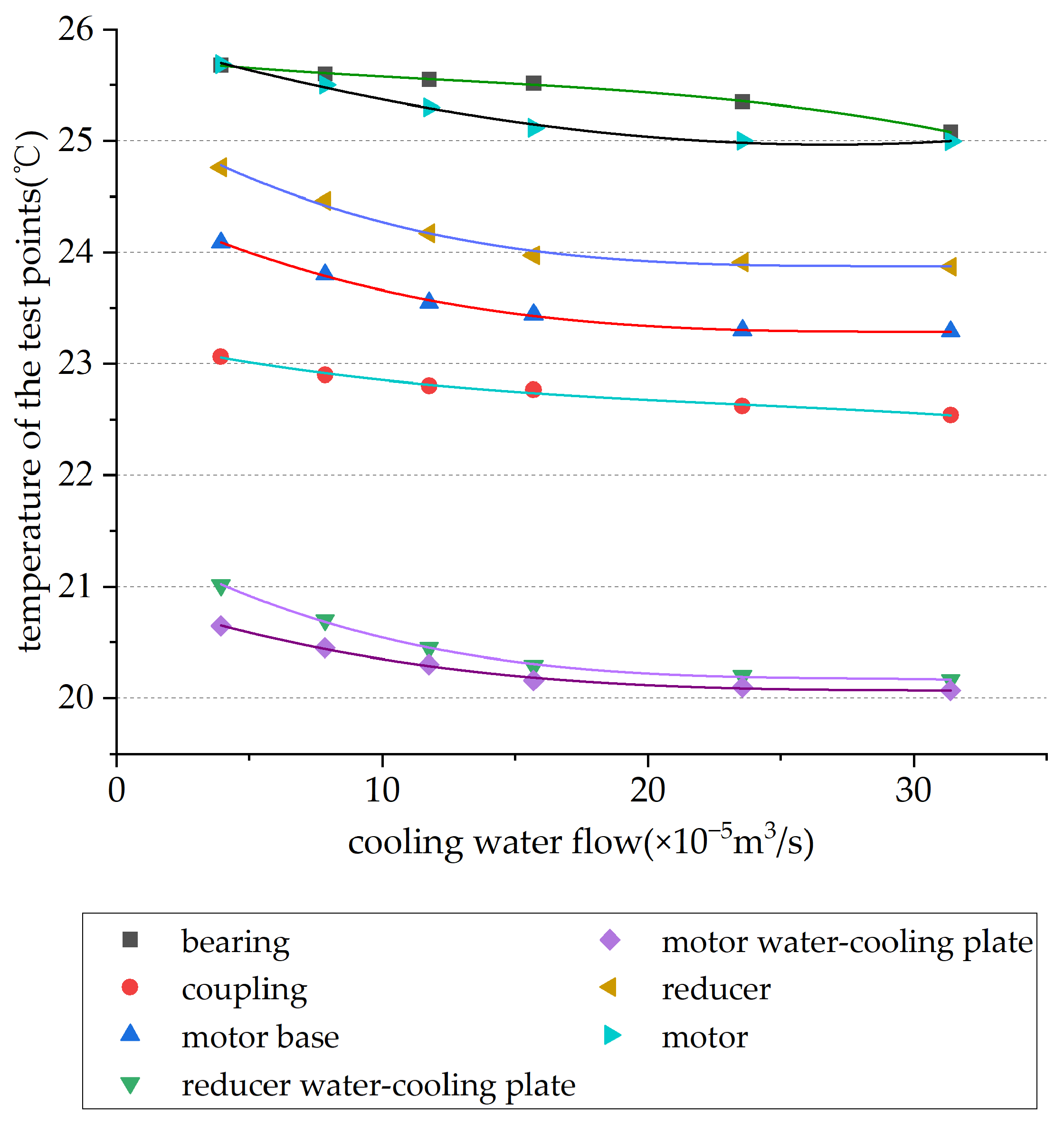
When using the simulation software to predict the influence of different flow rates on the temperature field of the whole machine, the range of cooling water flow rate was as follows: 3.925 × 10⁻⁵~3.14 × 10⁻⁴ m3/s, and the other simulation boundary conditions were as follows: motor speed: 2500 r/min, vacuum chamber temperature: 20 °C, cooling water temperature: 20 °C. Since different flows only affect the motor-reducer system, and then there were temperature changes on the Y-axis motor side bearing, coupling, motor base, and some beams, and there was no significant change on the temperature of other shafting of the whole machine, only the temperature changes of some parts were analyzed. Fitting the simulation results, the fitting functions of each temperature measuring point are shown in Table 7, where x is the flow, y is the component temperature, and the temperature fitting diagram is shown in Figure 18. It can be seen from the simulation results in Figure 16 that the temperature of parts had a turning point when the cooling water flow rate was 1.57 × 10⁻⁴ m3/s, and there was basically no significant drop when the flow was greater than 1.57 × 10⁻⁴ m3/s, and the temperature difference between the water-cooled plate and other parts was at least 2 °C.

Table 7.
Fitting function of temperature measurement points of each component under different flows.
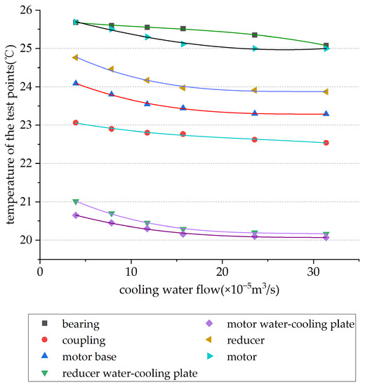
Figure 18.
Effect of different flow rates on the temperature of the test points.
5.2. The Temperature of the Whole Machine under Different Cooling Water Temperatures
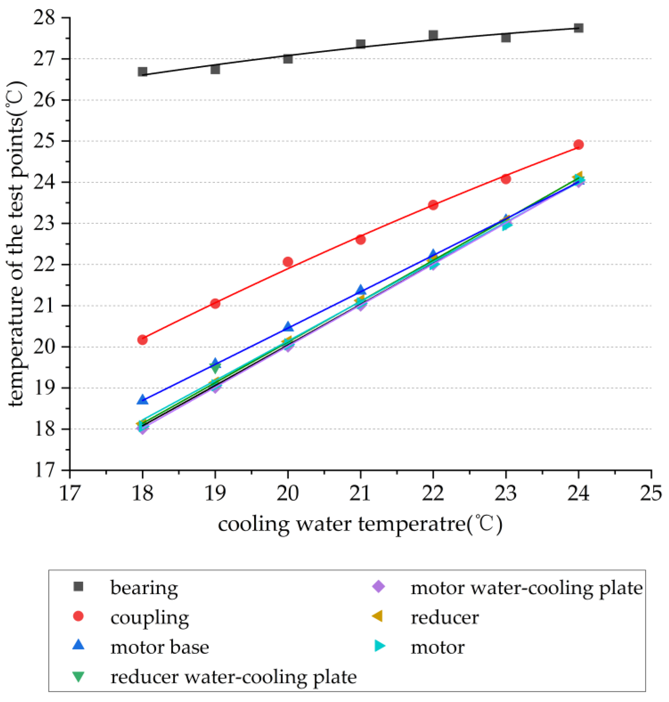
The simulation boundary conditions considering the influence of water-temperature change on the temperature field of the whole machine were as follows: motor speed: 2500 r/min, vacuum chamber temperature: 23.5 °C, cooling water flow: 1.57 × 10⁻⁴ m3/s, cooling water temperature: 18~24 °C. Similar to the previous section, only some parts had significant temperature changes. Fitting the simulation results, the fitting function of each temperature measuring point is shown in Table 8, where x is the cooling water temperature, y is the component temperature, and the temperature fitting diagram is shown in Figure 19. it can be seen that the bearing group was least affected by the water temperature, and the temperature increase was within 2 °C; the temperature of the other components was linearly related to the cooling water temperature. Except for the bearing group, the temperature difference of the other components was within 1 °C and tended to have the same temperature value.

Table 8.
Fitting function of temperature measurement points of components under different cooling water temperatures.
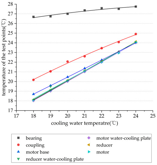
Figure 19.
The effect of different water temperatures on the temperature of test points.
5.3. Temperature of the Whole Machine at Different Motor Speeds
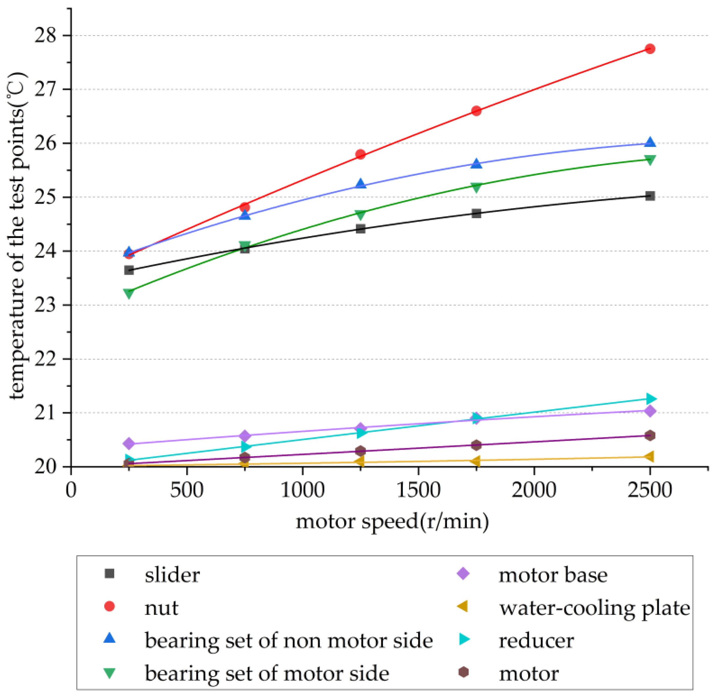
When the motor speed was 250~2500 r/min, the vacuum chamber temperature was 23.5 °C, the cooling water flow was 1.57 × 10⁻⁴ m3/s, and the cooling water temperature was 20 °C. Fitting the simulation results, the fitting functions of each temperature measuring point are shown in Table 9, where x is the motor speed, y is the component temperature, and the temperature fitting diagram is shown in Figure 20. The analysis of the simulation prediction values showed that the temperature difference between the motor-reducer system and the rest of the whole machine was about 3 °C due to the cooling effect of cooling water; when the speed was greater than 1250 r/min, the heat generated by the rest of the components except the nut was also absorbed. Part of the cooling water was taken away, the temperature remained stable, and the contact surface of the screw nut maintained a linear temperature increase.

Table 9.
Fitting function of temperature measurement points of various components at different motor speeds.
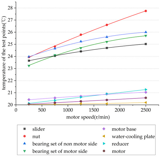
Figure 20.
The effect of different rotational speeds on the temperature of test points.
5.4. Temperature of the Whole Machine under Different Ambient Temperatures
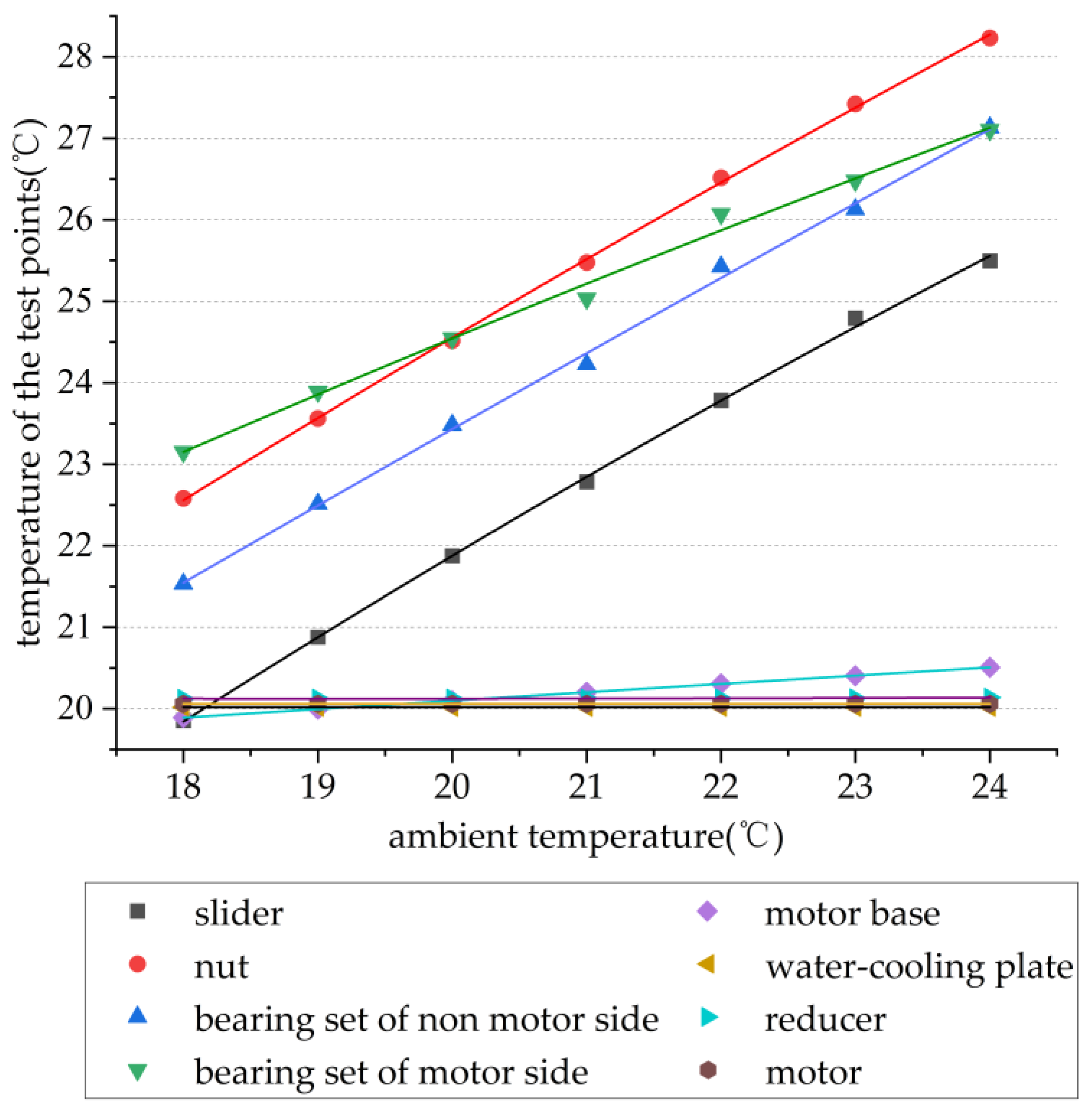
When the room temperature of the vacuum chamber was changed from 18 °C to 24 °C, and the remaining boundary conditions were as follows: the motor speed was 250 r/min, the cooling water flow was 1.57 × 10⁻⁴ m3/s, and the cooling water temperature was 20 °C. Fitting the simulation results, the fitting function of each temperature measuring point is shown in Table 10, where x is the cooling water temperature, y is the component temperature, and the temperature fitting diagram is shown in Figure 21. Under the action of cooling water, the temperature of the motor-reducer system was basically unaffected by the ambient temperature; the temperature of other components was linearly related to the temperature of the vacuum chamber.

Table 10.
Fitting function of temperature measurement points of each component under different ambient temperatures.
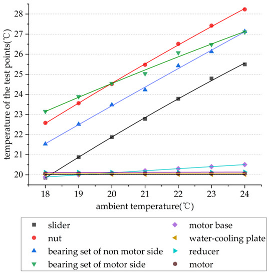
Figure 21.
Effect of different environments on the temperature of the test points.
Considering the cooling water flow rate, cooling water temperature, motor speed, and ambient temperature comprehensively, it can be seen that the cooling water temperature and flow rate had a greater impact on the motor-reducer system, and the temperature of the whole machine was relatively stable. There was a significant temperature gradient on the surface; the motor speed and ambient temperature had a great influence on the temperature distribution of the whole machine, and the two basically showed a linear distribution, and the cooling effect of the motor-reducer by the cooling water had no significant change.
6. Conclusions
Aiming at the identification of key parameters of thermal characteristics, thermal field analysis, and prediction of large machine tools under vacuum environments, this paper established a thermal characteristics simulation and calculation model, carried out the identification of key parameters based on experiments, completed the simulation analysis and verification of thermal characteristics of the whole machine, and provided the predicted data of thermal characteristics of machine tools. Specifically:
- (1)
- A new method for determining the heat-transfer coefficient was proposed. Through the combination of parametric simulation and experiment, the parameters of the heat-transfer coefficient were identified, and the heat-transfer coefficient between the motor and the water-cooled plate was determined to be 560 W/(m2∙°C); the heat-transfer coefficient between the reducer and the water-cooled plate was 510 W/(m2∙°C).
- (2)
- Through the simulation and test of the whole machine, the temperature field of the large machine tool in the vacuum environment was determined. When the cooling water temperature was 20.5 °C, the vacuum chamber temperature was 23.5 °C, and the motor speed was 250 r/min; the maximum temperature increase of 3 °C was at the bearing, the lowest temperature was at the water-cooling plate, and the temperature difference with the cooling water was within 0.5 °C.
- (3)
- The temperature increase prediction chart of the machine tool under different processing conditions such as cooling water flow rate, cooling water temperature, motor speed, and ambient temperature was provided. The chart can be used to determine whether the processing conditions are met according to specific processing requirements.
Author Contributions
Conceptualization, H.W.; methodology, T.L.; software, G.X.; validation, G.X., H.W. and W.T.; formal analysis, H.W.; investigation, G.X. and W.T.; resources, Z.S.; data curation, G.X. and X.S.; writing—original draft preparation, H.W.; writing—review and editing, X.S.; visualization, H.W.; supervision, T.L.; project administration, Z.S.; funding acquisition, T.L. and H.W. All authors have read and agreed to the published version of the manuscript.
Funding
This research is supported by Construction of High-level University—Leading Program of First-class Graduate Education (No.10-22-304-382, 10-22-304-393) and 2023 Shanghai Education Commission Young Teacher Training Subsidy Program.
Data Availability Statement
Not applicable.
Conflicts of Interest
The authors declare no conflict of interest.
References
- Temme, T.; Ostendorf, A.; Kulik, C. Machining of optical microstructures with 157 nm laser radiation. In Proceedings of the Fourth International Symposium on Laser Precision Microfabrication, Munich, Germany, 21–24 June 2003; International Society for Optics and Photonics: Bellingham, MA, USA, 2003. [Google Scholar]
- Wang, X. Effect of Quasi-Vacuum Environment in Ablation with High Repetition Rate Pulsed Laser. Chin. J. Lasers 2009, 36, 238–243. [Google Scholar] [CrossRef]
- Lai, K.; Cao, H.; Li, H.; Li, B.; Huang, D. Coupling evaluation for material removal and thermal control on precision milling machine tools. Front. Mech. Eng. 2022, 17, 13. [Google Scholar] [CrossRef]
- Al-Damook, A.; Summers, J.L.; Kapur, N.; Thompson, H. Effect of temperature-dependent air properties on the accuracy of numerical simulations of thermal airflows over pinned heat sinks. Int. Commun. Heat Mass Transf. 2016, 78, 163–167. [Google Scholar] [CrossRef]
- Laraqi, N.; Bairi, A. Theory of thermal resistance between solids with randomly sized and located contacts. Int. J. Heat Mass Transf. 2002, 45, 4175–4180. [Google Scholar] [CrossRef]
- Meng, Q.; Yan, X.; Sun, C.; Liu, Y. Research on thermal resistance network modeling of motorized spindle based on the influence of various fractal parameters. Int. Commun. Heat Mass Transf. 2020, 117, 104806. [Google Scholar] [CrossRef]
- Chen, M.; Li, Q.; Zhang, P. Experimental investigation of high temperature thermal contact resistance of thin disk samples using infrared camera in vacuum condition. Int. J. Heat Mass Transf. 2020, 157, 119749. [Google Scholar] [CrossRef]
- Mori, K.; Kono, D.; Matsubara, A. Effect of expansion coefficient difference between machine tool and workpiece to the thermal deformation induced by room temperature change. Procedia CIRP 2021, 101, 318–321. [Google Scholar] [CrossRef]
- Liu, J.; Cai, Y.; Zhang, Q.; Zhang, H.; He, H.; Gao, X.; Ding, L. Thermal error analysis of tauren EDM machine tool based on FCM fuzzy clustering and RBF neural network. J. Intell. Fuzzy Syst. Appl. Eng. Technol. 2021, 41, 6003–6014. [Google Scholar] [CrossRef]
- Zhang, P.; Cui, T.; Li, Q. Effect of surface roughness on thermal contact resistance of aluminium alloy. Appl. Therm. Eng. 2017, 121, 992–998. [Google Scholar] [CrossRef]
- Duo, R.; Ge, T.; Liu, X. Effects of contact pressure, interface temperature, and surface roughness on thermal contact conductance between stainless steel surfaces under atmosphere condition. Int. J. Heat Mass Transf. 2016, 94, 156–163. [Google Scholar]
- Sun, F.; Zhang, P.; Wang, H.; Shen, J.; Nie, L. Experimental study of thermal contact resistance between aluminum alloy and ADP crystal under vacuum environment. Appl. Therm. Eng. 2019, 155, 563–574. [Google Scholar] [CrossRef]
- Tian, J. Thermal Properties Analysis and Experimental Study of Large-Scale Moving Platform in Vacuum Environment. Master’s Thesis, Harbin Institute of Technology, Harbin, China, 2020. [Google Scholar]
- Chen, Y.; Feng, S.; Li, X. Effect of interface morphology on thermal contact resistance in thermal management of electronic devices. Int. J. Mod. Phys. B 2022, 36, 2250092. [Google Scholar] [CrossRef]
- Nishino, K.; Yamashita, S.; Torii, K. Thermal contact conductance under low applied load in a vacuum environment. Exp. Therm. Fluid Sci. 1995, 10, 258–271. [Google Scholar] [CrossRef]
- Ding, C.; Wang, R. Thermal contact conductance of stainless steel-GFRP interface under vacuum environment. Exp. Therm. Fluid Sci. 2012, 42, 1–5. [Google Scholar] [CrossRef]
- Dongmei, B.; Chen, H.; Ye, T. Influences of temperature and contact pressure on thermal contact resistance at interfaces at cryogenic temperatures. Cryogenics 2012, 52, 403–409. [Google Scholar]
- Chen, B.; Guan, X.; Cai, D.; Li, H. Simulation on thermal characteristics of high-speed motorized spindle. Case Stud. Therm. Eng. 2022, 35, 102144. [Google Scholar] [CrossRef]
- Weng, L.; Gao, W.; Zhang, D.; Huang, T.; Liu, T.; Li, W.; Zheng, Y.; Shi, K.; Chang, W. Analytical modelling method for thermal balancing design of machine tool structural components. Int. J. Mach. Tools Manuf. 2021, 164, 103715. [Google Scholar] [CrossRef]
- Liu, D.; Zhang, J. Numerical simulation of high-temperature thermal contact resistance and its reduction mechanism. PLoS ONE 2018, 13, e0194483. [Google Scholar] [CrossRef]
- Li, Z.; Chen, B. Design and analysis of lunar-based tracking turntable for earth observation. Acta Photonica Sin. 2010, 39, 2215–2219. [Google Scholar]
- Min, X.; Jiang, S. A thermal model of a ball screw feed drive system for a machine tool. J. Mech. Eng. Sci. 2011, 1, 1–8. [Google Scholar] [CrossRef]
- Wu, C.; Kung, Y. Thermal analysis for the feed drive system of a CNC machine center. Int. J. Mach. Tools Manuf. 2003, 43, 1521–1528. [Google Scholar] [CrossRef]
Publisher’s Note: MDPI stays neutral with regard to jurisdictional claims in published maps and institutional affiliations. |
© 2022 by the authors. Licensee MDPI, Basel, Switzerland. This article is an open access article distributed under the terms and conditions of the Creative Commons Attribution (CC BY) license (https://creativecommons.org/licenses/by/4.0/).


