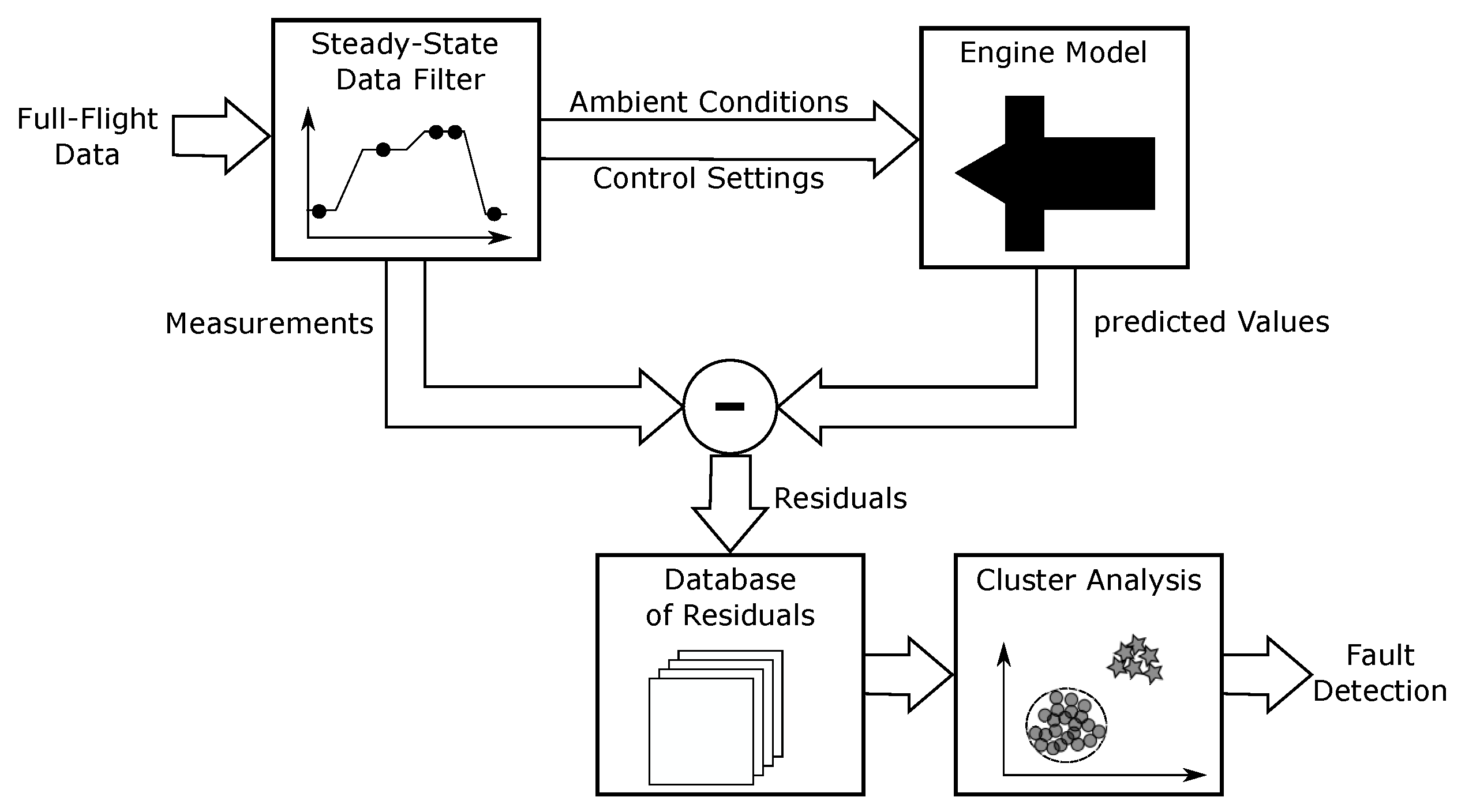
The generation of residuals requires the in-flight measurements to fulfill the prerequisites for applying steady-state performance models, i.e., constant flight and ambient conditions, constant engine control settings, and engine offtakes. Additionally, the engine must have reached thermal equilibrium. The first four aspects are summarized as a stable operating regime, and the latter represents a thermal stability criterion.
Of the approaches presented in
Section 2.3, only the approach described by [
40] explicitly covers all of these aspects. In order to meet the prerequisites of stable operating regimes and thermal stability, the Steady-State Data Filter consists of four building blocks: a Low-Pass Filter, a Thermal Transient Filter, a Regime Recognition, and a State Transition Logic. A flowchart of the resulting Steady-State Data Filter is visualized in
Figure 2. Since the algorithm of [
40] was derived for identifying steady-state data points for turboshaft engines of helicopters, some adjustments are needed to apply the approach to turbofan engines of commercial aircraft.
3.2.1. Low-Pass Filter
Due to measurement noise, the total number of detected steady-state data points might significantly differ from engine to engine, even if they are both mounted on the same aircraft [
40]. A low-pass filter is proposed for alleviating the effect of high-frequency noise in the input signal. In general, the response of a low-pass filter can be characterized by its cut-off frequency and order. The cut-off frequency defines the beginning of the signal attenuation, and the magnitude of the attenuation is directly dependent upon the order of the filter [
50].
The filter has to be designed such that mostly the high-frequency measurement noise is attenuated, leaving the remaining frequency spectrum unaffected. The measurement noise depends on the type of sensors used, their dynamics, and the data acquisition. Since the measurement systems in turboshaft engines and turbofan engines for commercial aircraft are expected to be similar, the filter defined by [
40] is directly adopted. Hence, a second-order low-pass filter is implemented where
is the raw and
is the corresponding low-pass filtered measurement.
An adjustment concerning the position of the low-pass filter is proposed. In the original algorithm, the Low-Pass Filter works in parallel with both the Thermal Transient Filter and the Regime Recognition. A low noise level is expected to be advantageous for determining thermally stable flight segments and the definition of valid flight segments. Hence, utilizing the Low-Pass Filter as a preprocessing step is considered more suitable.
3.2.2. Thermal Transient Filter
The Thermal Transient Filter is used to assure the thermal equilibrium of the engine. Since the time required to heat through an engine generally correlates with its mass [
51], the definition of the Thermal Transient Filter has to be adjusted in order to account for the application in commercial turbofan engines.
For approximating the heat fluxes of the engine, a simplified thermal model is evaluated approximating the multi-stage components by representative single-stage modules according to [
52]. Such a simplified module is visualized in
Figure 3. The thermal model takes the heat fluxes between fluid and casing
, fluid and blade
, and disk and blade
into account. Single elements approximate all structural elements, and the module is approximated as adiabatic. The heat fluxes between the structural elements and the fluid
and
are modeled assuming convective heat transfer. A conductive heat transfer is assumed for the heat fluxes between disk and blade
. The heat fluxes are defined based on the heat transfer coefficients
, the wetted area
A, and the temperatures of the fluid and structural elements
T.
Conductive heat transfer within the structural elements is neglected, assuming an instantaneously uniform temperature distribution within the material. The corresponding temperature changes of the structures can be evaluated via conservation of energy using the mass of the structure
m, and the heat capacity of the material
cSubstituting Equation (
2) into Equation (
3) finally yields a system of first-order differential equations for the temperatures of the casing, disks, and blades of the module.
Applying a Laplace transformation to the first-order differential equation of the casing in Equation (
4) results in
Equation (
8) is of similar form as the first-order filter proposed by [
40] for approximating thermal equilibrium within the Thermal Transient Filter. Here, a similar first-order filter is used to describe the correlation between the filtered exhaust gas temperature
and its raw measurement
with a given time constant
Comparing Equation (
8) and Equation (
9) shows that
characterizes the heat transfer. In general, the lower
, the faster the temperature response of the material to a step change of the fluid temperature.
For utilizing the Thermal Transient Filter a representative time constant
has to be defined approximating the heat exchange of a particular engine model. The time constants are computed based on Equations (4)–(7). The mass
m, heat capacity
c, and wetted area
A are approximated from drawings and material datasheets. In general, the heat transfer coefficient
depends on the geometry, fluid properties, and flow properties. Consequently, the time constant
is not fixed but varies with power-setting. Here, a Nusselt-Correlation is used for approximating the heat transfer coefficients
[
53] with the Reynolds-Number
, the Prandtl-Number
, the characteristic length
l, and the thermal conductivity of the fluid
.
In order to avoid the necessity to recompute the heat transfer coefficients
constantly for changing power settings, the slowest possible heat transfer encountered during operation is used as a conservative estimate. Simplifying Equation (
10) yields approximately
. Hence, a low-idle power-setting results in the highest time constants
due to the low corresponding Reynolds-Numbers. For evaluating the thermal model, the material properties and dimensions of the components are derived based on an existing and validated model by [
52]. The resulting time constants
for the different modules in a low idle-setting are summarized in
Table 1. No thermal model is utilized for the fan and LPC since the heat fluxes are considered negligible. Based on
Table 1, the largest time constant is selected for the Thermal Transient Filter as
s.
Since Equation (
9) defines a first-order differential equation, appropriate initial conditions have to be defined for the filtered EGT. The initial thermal state of the engine is directly dependent upon its flight history [
52]. Therefore, it cannot be determined without analyzing the preceding flight. In order to avoid such an extensive analysis, the filtered EGT is initialized with the ambient temperature resulting in a conservative estimate of the material temperature, assuming the engine was completely cooled down.
According to [
40] a thermally stabilized state is defined if the difference between the filtered and unfiltered EGT is below a threshold of
K, selected to be at the same order of magnitude as the EGT measurement uncertainty [
16,
17].
3.2.4. State Transition Logic
The State Transition Logic defines a steady-state regime if the low-pass filtered data fulfill the requirements of the Thermal Transient Filter as well as the Regime Recognition, and the variance of the filtered data is below a threshold value within a given moving window of length
. Its primary purpose is to ensure that the steady-state data points fulfill the requirements of a steady-state performance synthesis calculation, i.e., the stability of the flight conditions, power-setting, thermal state, and mechanical state. The approach defined by [
41] is used, which allows the direct definition of limits on the relevant measurements. The maximum variations
D of the measurements
y are defined as the min-max range
The maximum variations of the parameters summarized in
Table 2 are monitored for ensuring stable flight conditions. The values are application-dependent and were chosen to limit the difference of both net thrust and stored energy. The maximum variation chosen for the parameters related to stable flight conditions ensures that the net thrust in altitude varies with less than 0.5%. The maximum variation of parameters related to the mechanical equilibrium ensures that the power stored in rotating structures varies with less than 5%. The maximum variation of the power setting parameter can be defined based on the measurement uncertainty of aircraft fuel meters [
54].
If all stability conditions are met, the corresponding data points within the moving window are arithmetically averaged, resulting in a steady-state data point. The population of the residuals between those steady-state data points and the corresponding predicted values of an engine model forms the input to the following clustering approach.


 ,
, 


