Article

Theoretical and Simulation Analysis on Fabrication of Micro-Textured Surface under Intermittent Cutting Condition by One-Dimensional Ultrasonic Vibration-Assisted Turning

1
School of Mechanical Engineering, Shandong University of Technology, Zibo 255000, China
2
Key Laboratory of High Efficiency and Clean Mechanical Manufacture, Ministry of Education of China, School of Mechanical Engineering, Shandong University, Jinan 250061, China
3
College of Mechanical and Electronic Engineering, Shandong University of Science and Technology, Qingdao 266590, China
*
Author to whom correspondence should be addressed.
Machines 2022, 10(3), 166; https://doi.org/10.3390/machines10030166
Submission received: 12 January 2022 / Revised: 15 February 2022 / Accepted: 18 February 2022 / Published: 22 February 2022
(This article belongs to the Section Friction and Tribology)

Abstract

:
Fabricating micro-textures with specific parameters (size, shape, and distribution) on the surface of mechanical components has the potential to improve the tribological performance. When the ultrasonic vibration is applied to depth direction of turning, the micro-textured surfaces with specific dimples can be generated in a simple and effective way. Under the intermittent cutting condition, the generation mechanism of the micro-textured surface, processed by this one-dimensional ultrasonic vibration-assisted turning (1D UVAT), was further carried out. A novel theoretical model was firstly proposed from the perspective of geometric kinematics, which can reveal the influence of three intersection states between the flank face and cutting trace (η1 < tan α, η1 > tan α > η2 and η2 > tan α) on the size, shape, and distribution of micro-dimples, generated under intermittent cutting conditions. Then, a simulation model was built to predict the surface topography and dimple profile under different processing parameters. The results show that the processing parameters, including clearance angle, spindle speed, and vibration amplitude, have an important influence on the intersection state. By choosing the proper clearance angle, spindle speed, or vibration amplitude, the different intersection states can be realized, and the corresponding size, shape, and distribution of micro-dimples will be changed accordingly. With the increase of the nose radius and feed rate, the dimple width and distance between adjacent dimples along feed direction can both increase accordingly. The simulation results not only confirm the feasibility of the proposed theoretical model, but also show that the discrete or continuous micro-dimples, with different sizes and specific shapes, can be controllably generated on cylindrical surface by 1D UVAT under intermittent cutting conditions.

1. Introduction

In recent years, the micro-textured surfaces have gained widespread research and applications in various engineered fields, due to their good tribological performance [1,2,3,4]. The texture shapes on surface mainly include dimple, groove, convex, etc. Among them, dimple is the most commonly used texture shape. The textured surfaces with micro-dimples have been applied in many lubricated applications, such as seals, journal bearings, piston rings, etc. [5,6,7,8]. The micro-dimples with specific distribution, size, and shape on surface of tribo-pairs can act as a lubricant reservoir, which provides lubricant for the contact area, in case of starved lubrication [9,10], entrap wear debris during the friction process [9,11,12], decrease the contact area to reduce stiction [13], and produce an additional hydrodynamic lift, in order to improve the load-carrying capacity of the contact area under mixed and hydrodynamic lubrication [2,14].
In order to achieve the fabrication of micro-textured surface, many processing technologies have been proposed, such as laser surface texturing (LST) [9,10,12,13,14,15], LIGA [16], chemical etching [17], electrical discharge texturing (EDT) [18], abrasive-jet machining (AJM) [19], and micro-forming [20]. Though every method has its own processing characteristic and application range of materials, it is still necessary for the present to develop more simple, cost-effective, and efficient surface texturing technology for mass production [21].
Ultrasonic vibration-assisted turning (UVAT) is a kind of composite machining method, which is realized by applying ultrasonic vibration to the conventional turning. Through changing cutting trace and material removal mechanism, the UVAT can achieve obvious advantages in improving surface quality [22], machining difficult-to-machine material [23,24], and reducing cutting force [25]. Based on the specific characteristic of vibration cutting process, the UVAT has also been applied to fabricate micro-textured surfaces in recent years, including the 1D UVAT and elliptical UVAT [26,27]. As for the elliptical UVAT, the ultrasonic vibration needs to be applied to two vertical directions of turning, and the corresponding vibration locus is elliptical. Compared with the elliptical UVAT, the ultrasonic vibration device (UVD) used for 1D UVAT is much easier to design and realize. When the ultrasonic vibration is applied to the depth direction of turning, the micro-dimples can be generated on cylindrical and end surfaces, which has been proved to be a simple and efficient way for surface texturing. As for this kind of 1D UVAT, there are two processing conditions, including the continuous cutting and intermittent cutting conditions. Liu et al. have systematically studied the effects of processing parameters, under continuous cutting conditions, on the distribution, size, and shape of micro-dimples, through theoretical analysis, simulation prediction, and experimental verification, and revealed that the intersection state between flank face and cutting trace has an important impact on the generation of micro-dimples [28,29,30]. However, the 1D UVAT under continuous cutting conditions can only fabricate continuous micro-dimples on the surface. In order to change the continuous micro-dimples to the discrete micro-dimples, under continuous cutting conditions, the cutting tool without ultrasonic vibration needs to machine the workpiece surface again after the UVAT process [31], and this way also makes the texturing process complicated, in turn. Different from the micro-dimples fabricated under continuous cutting conditions, the 1D UVAT under intermittent cutting conditions can not only generate continuous micro-dimples, but also directly fabricates discrete micro-dimples on the surface, which provides more selection for the fabrication of various micro-dimpled surface. However, for the 1D UVAT under intermittent cutting conditions, there is still a lack of more systematical study on the corresponding generation mechanism and features of micro-textured surface. In order to further reveal the generation mechanism and features of micro-textured surface, fabricated by 1D UVAT under intermittent cutting conditions, this paper proposes a novel theoretical model, from the perspective of geometric kinematics, which can reveal the key factors affecting the generation of discrete or continuous micro-dimples for the first time. Based on the proposed theoretical model, the influence of three intersection states between the flank face and cutting trace (η1 < tan α, η1 > tan α > η2 and η2 > tan α) on the size, shape, and distribution of the micro-dimples generated under intermittent cutting conditions can be systematically explored. Besides, this paper will also establish a simulation model to predict the micro-textured surface topographies and dimple profiles under different processing parameters and confirm the theoretical model. Therefore, this paper will study the effects of processing parameters on the distribution, size, and shape of micro-dimples fabricated by the 1D UVAT under intermittent cutting conditions through theoretical and simulation analysis.

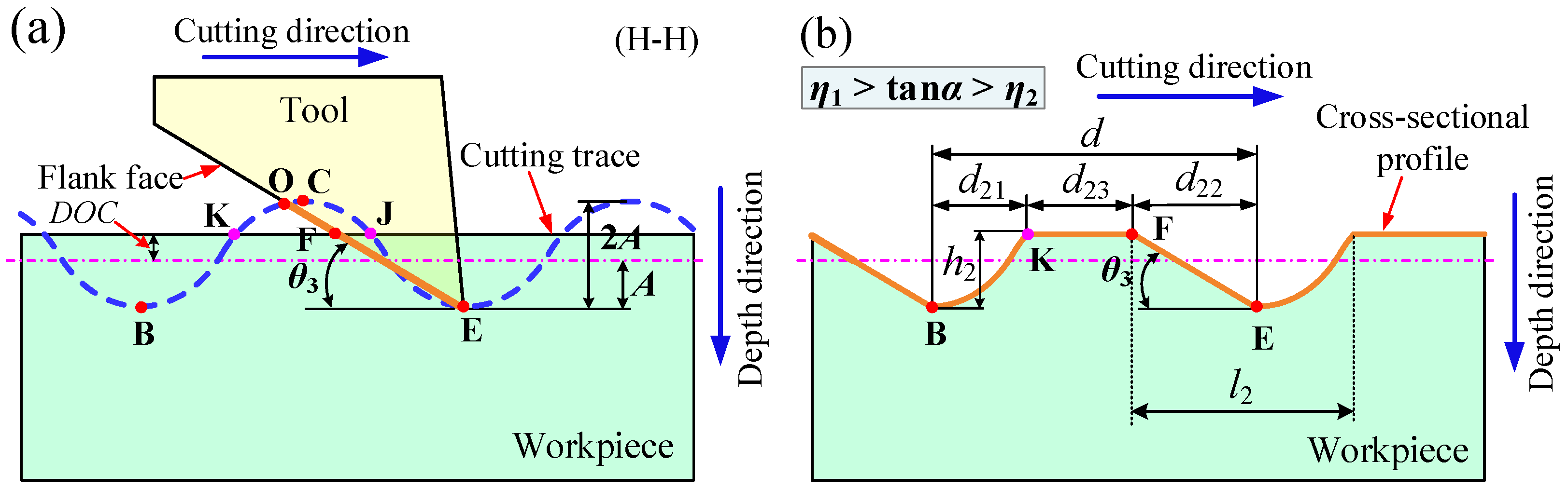
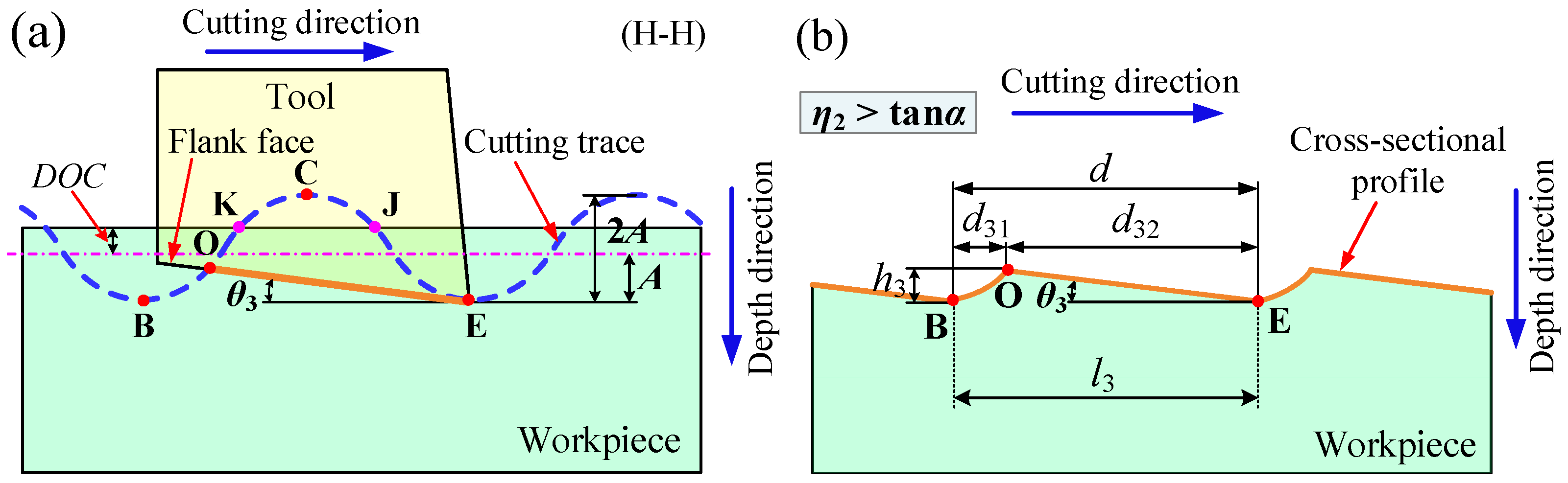
2. Theoretical Analysis

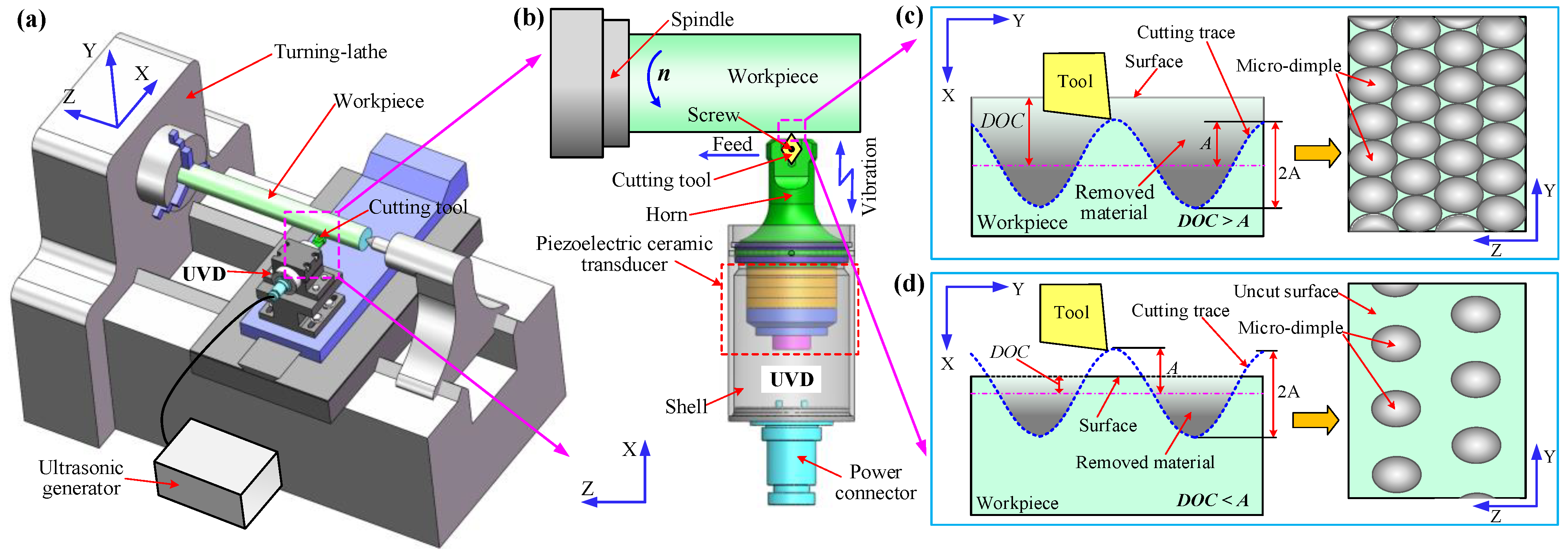
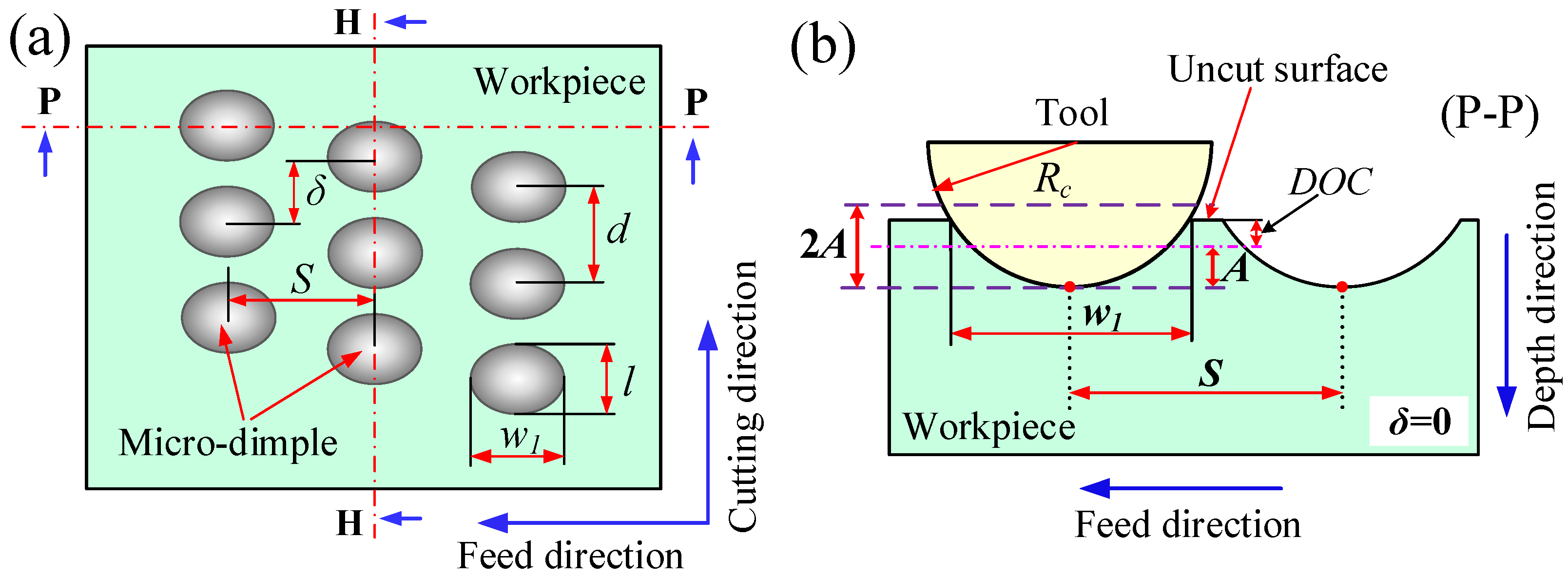
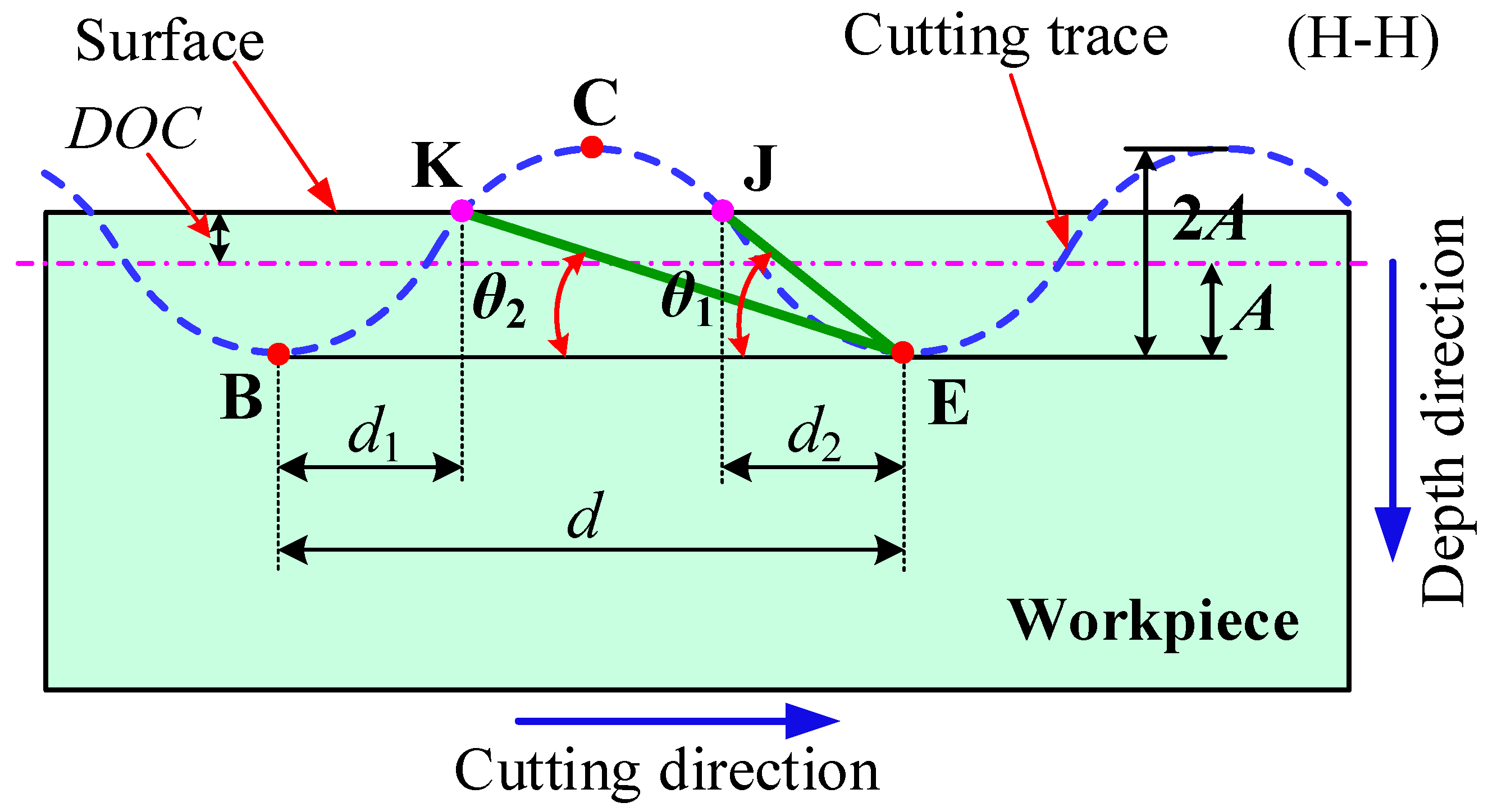
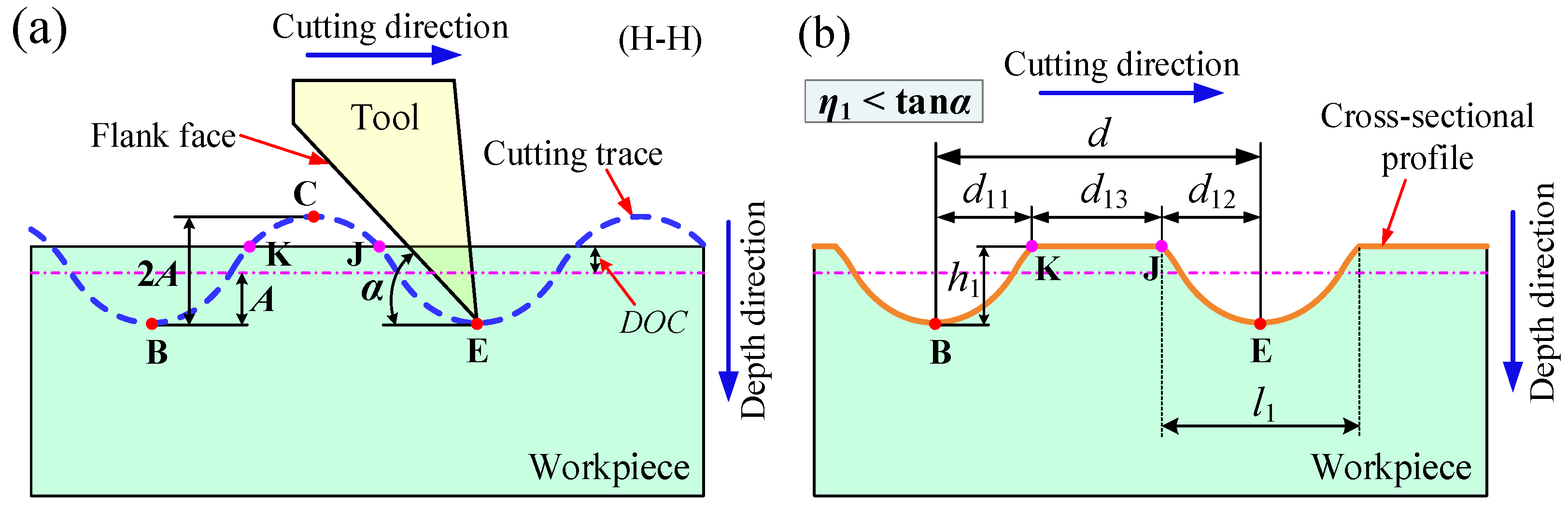
2.1. Surface Texturing Process

The surface texturing process of 1D UVAT under continuous and intermittent cutting conditions can be detailedly described in Figure 1, among which, the coordinate axes of X, Y, and Z represent the depth, cutting, and feed directions, respectively. The overall assembly drawing of equipment for 1D UVAT can be seen in Figure 1a. The workpiece, which can rotate with the spindle, is mounted on a turning-lathe through the chuck and top cone. The UVD, used for 1D UVAT, is mounted on the sliding table of turning-lathe through a designed base. The UVD mainly includes a piezoelectric ceramic transducer, horn, shell, and power connector, as shown in Figure 1b. The piezoelectric ceramic transducer is used to convert electrical signal into vibration. The horn has the function of magnifying the vibration. The cutting tool is mounted to the front end of horn of the UVD. The ultrasonic generator provides the power for UVD, and the cutting tool can make a sinusoidal reciprocating motion in the depth direction. Therefore, the cutting tool can not only move in the X and Z directions, but also can make a sinusoidal reciprocating motion in the X direction.
For the 1D UVAT, the continuous cutting condition is that the depth of cut (DOC) is larger than ultrasonic vibration amplitude (A), that is DOC > A, and the micro-dimples fabricated under this condition connect each other on surface, which can be seen in Figure 1c. As for the intermittent cutting condition, the depth of the cut is less than the ultrasonic vibration amplitude, that is DOC < A, as shown in Figure 1d. It can be found that the sinusoidal cutting trace can be formed in the XY plane, and the cutting tool can intermittently cut the workpiece surface, resulting the formation of micro-dimples. The distribution and geometry characteristics of micro-dimples fabricated under intermittent cutting conditions will be different from that fabricated under continuous cutting conditions. Except for the continuous micro-dimples, the discrete micro-dimples also can be generated on cylindrical surface under intermittent cutting conditions, as shown in Figure 1d.
According to our previous studies [28,29,30], the corresponding output of vibration amplitude of UVD is smaller than 10 μm. Therefore, for the 1D UVAT, the DOC should be less than 10 μm, in order to meet the intermittent cutting conditions, and the selected turning-lathe should be a high precision lathe in this study. However, the minimum resolution in the depth direction and repetitive positioning accuracy of the existing CNC lathe (CKD6150H, Precion, Dezhou, Shandong, China), used in the previous study, were all 5 μm, which is hard to satisfy the accuracy requirements for the intermittent cutting process. Due to the limited experimental conditions for the 1D UVAT under intermittent cutting conditions, the corresponding experimental tests for this paper will not be conducted for the time being, and the paper mainly researches the generation mechanism and features of micro-textured surfaces, from the perspective of theoretical and simulation analysis. Certainly, the experimental verification will be carried out in the future, when a suitable precision turning-lathe is ready.

2.2. Theoretical Model

Figure 2 depicts the illustration of micro-textured surfaces, generated under intermittent cutting conditions, including the arrangement and geometry of micro-dimples and cross-sectional dimple profiles along feed direction. According to Figure 2a, the arranged discrete micro-dimples can be formed on the workpiece surface. The important factors influencing the shape, size, and distribution of micro-dimples include w1 (dimple width along feed direction), l (dimple length along cutting direction), S (distance between adjacent dimples along feed direction), d (distance between adjacent dimples along cutting direction), and δ (phase-shift distance of adjacent dimples).
The distance between adjacent dimples along the feed direction, S, is determined by the feed rate, which can be expressed as follows:
S = f
where f is the feed rate. Therefore, the feed rate has an important influence on the distribution density of micro-dimple along feed direction. The distance between adjacent dimples along cutting direction, d, is equal to the cutting distance of one vibration cycle [28,29], which can be calculated from:
d = v c / f u s = π R n 30 f u s
where vc is the cutting speed (mm/s), fus is the vibration frequency, R is the radius of workpiece, and n is the spindle speed (rev/min). As for the phase-shift distance of the adjacent dimples, the detailed description and calculation can be found in references [28,29].
When δ = 0 and S > w1, the dimple width, as indicated by the cross-section pp in the feed direction, is shown in Figure 2b. It can be seen that the adjacent dimples, along the feed direction, are in discrete status, and the overlapping part does not exist between the adjacent dimples. Under this condition, the dimple width can be expressed by the following:
w 1 = 2 R c 2 ( R c D O C A ) 2
where Rc is the nose radius of cutting tool. Therefore, the dimple width is determined by parameters including nosed radius, depth of cut, and vibration amplitude.
Under the intermittent cutting condition, the cutting trace on XY plane, as indicated by the cross-section hh in cutting direction, is detailedly described in Figure 3. In a vibration period, the cutting tool moves along cutting trace from bottom point B, through the point K and then away from the workpiece surface to reach the vertex C. After point C, the cutting tool then moves through point J to reach the bottom point (E). Thus, it can be seen that the BK and JE segments belong to the cutting stage of workpiece material, and the KJ segment belongs to the non-cutting stage of workpiece material. The distance in cutting direction of BK segment is defined to be d1, and the distance in cutting direction of JE segment is defined to be d2, as shown in Figure 3. It can be found that the BK and JE segments of the cutting trace are symmetrically distributed around vertex C. Therefore, the d1 is equal to the d2. The angle between JE and BE is θ1, and the angle between KE and BE is θ2. The tangent values of θ1 and θ2 are defined to be the intersecting rates η1 and η2, respectively, which can be expressed by the following:
η 1 = tan   θ 1 = D O C + A d 2
η 2 = tan   θ 2 = D O C + A d d 1
Since the d1 and d2 are equal, only the distance d1 is calculated; the values of η1 and η2 can be obtained by the Equations (4) and (5).
In order to calculate d1, the sinusoidal cutting trace in the XY plane is placed in a new X′-Y′ coordinate system, as shown in Figure 4. The X′ axis is the opposite direction of X axis, and the Y′ axis is consistent with Y axis. The Y′ axis represents not only the displacement value along Y direction but also the time axis. That is, the value of Y′ axis also corresponds to a time point t. In Figure 4, the T represents a period of ultrasonic vibration, which can be expressed by the following:
T = 1 f u s
Therefore, the sinusoidal cutting trace, varying with time, can be expressed as:
X = A sin   ( 2 π f u s t π / 2 ) + A
As shown in Figure 4, the time point corresponding to the d1 is t1, which is the time taken for the cutting tool moving from point B, along the cutting trace, to point K. The value of X′ axis corresponds to t1 is DOC + A. By introducing the t1 and DOC + A into the Equation (7), it can get the following equation:
D O C + A = A sin   ( 2 π f u s t 1 π / 2 ) + A
Consequently, the t1 can be further calculated by the following:
t 1 = a r c sin   ( D O C A ) + π 2 2 π f u s
Through bringing the calculated value of t1 into the following equation, the value of d1 can be obtained.
d 1 = v c t 1 = π R n t 1 30
It can be seen from the above equations that the major factors influencing η1 and η2 are DOC, n, A, fus, and R. During this surface texturing process, the intersection state between the flank face and cutting trace is the key factor to determine the distribution, size, and shape of the micro-dimples in cutting direction. As an important tool parameter, the clearance angle (α) plays a significant role in this process.
For further simplifying of the theoretical model, the elastic–plastic deformation of workpiece material in the UVAT process has not been considered in this paper. The paper mainly studies the relationships of flank face and cutting trace from the perspective of geometric kinematics and analyses the size and shape of dimples under three intersection states.
As shown in Figure 5a, when tool moves along cutting trace, the flank face has no intersection with the cutting trace, that is, η1 < tan α, which can be considered to be the first state. Under this state, the cross-sectional profile of dimples in cutting direction can be seen from the Figure 5b. It can be seen that the flank face has no effect on the dimple profile which is only related to the cutting trace. The adjacent dimple profile is discrete. There is a distance d13 in the middle, which belongs to the uncut surface. Under this state, the dimple depth h1 can be expressed by the following:
h 1 = D O C + A
The distance between adjacent dimples along cutting direction includes three parts, d11, d13, and d12. Due to the symmetry between BK and JE, relative to point C, d11, and d12 are equal, which are also equal to d1 and d2, respectively. Therefore, the dimple length along cutting direction can be calculated by the following:
l 1 = d 11 + d 12 = 2 d 1
As shown in Figure 6a, when the tool moves along cutting trace to point E, the flank face intersects with the KJ segment of the cutting trace on point O, that is, η1 > tan α > η2, which can be considered to be the second state. Under this state, the flank face intersects with the workpiece surface on the F point. The angle between OE and BE is θ3, which is equal to the clearance angle of tool. The cross-sectional profile of the dimples in the cutting direction can be seen form Figure 6b. The adjacent dimples in the cutting direction are still discrete, and a distance d23, corresponding to the uncut surface, also exists between the adjacent dimple profiles. Because of the intersection between the flank face and cutting trace, a part of dimple profile can be approximated by the FE segment. The corresponding length d22 also changes, which can be calculated by the following:
d 22 = D O C + A tan   θ 3 = D O C + A tan   α
Under this state, the distance between the adjacent dimples along the cutting direction includes three parts, d21, d23, and d22. The d21 is equal to the d1, and the dimple depth h2 is consistent with the dimple depth h1, which can be also expressed by the following:
h 2 = h 1 = D O C + A
The dimple length along cutting direction can be calculated by the following:
l 2 = d 21 + d 22
As shown in Figure 7a, when tool moves along the cutting trace to reach point E, the flank face intersects with the BK segment of the cutting trace on point O, that is, η2 > tan α, which can be considered to be the third state. The cross-sectional profile of the dimples is shown in Figure 7b. For the third state, the generation process of the micro-dimples is similar to that under the continuous cutting condition. The distance between adjacent dimples along cutting direction is equal to the dimple length l3, including two parts of d31 and d32, which can be obtained from the following:
l 3 = d 31 + d 32
Because the cross-point O on BK segment is below the workpiece surface, the dimple depth h3 is different from that of the first two states. In order to facilitate the calculation of h3, the sinusoidal cutting trace, varying with time under the state of η2 > tan α, is firstly expressed in Figure 8. The value of the Y′ coordinate corresponding to point O is d31, as well as the corresponding time point, is t31. The d31 can be calculated by the following:
d 31 = v c t 31
Therefore, the d32 can be expressed by:
d 32 = d d 31
The dimple depth h3 can be formulated by the following:
h 3 = d 32 tan   θ 3 = d 32 tan   α
In addition, according to Equation (7), the dimple depth h3 can also be formulated by the following:
h 3 = A sin   ( 2 π f u s t 31 π / 2 ) + A
Consequently, by combining the Equations (17)–(20), the value of t31 can be firstly calculated. Then, the dimple depth h3 will be obtained, according to the Equation (20).
Based on the above theoretical analysis, the intersection state can greatly influence the dimple profile in the cutting direction, which, in turn, affects the distribution, size, and shape of micro-dimples. The illustration of the dimple shape, under different states, can be seen in Figure 9. Under the states of η1 < tan α and η1 > tan α > η2, the dimples along cutting direction are discrete, showing different degrees of ellipse. For the first state, the shape of single micro-dimple is symmetrical, up and down, along the cutting speed. For the second state, however, the shape of single micro-dimple is asymmetric along the cutting direction. When η2 > tan α, the adjacent dimples are continuous. The shape of single micro-dimple becomes scaly-like and more asymmetric along the cutting direction. Therefore, by choosing the proper processing parameters to change the intersection state, the micro-dimples with specific characteristics can be fabricated.

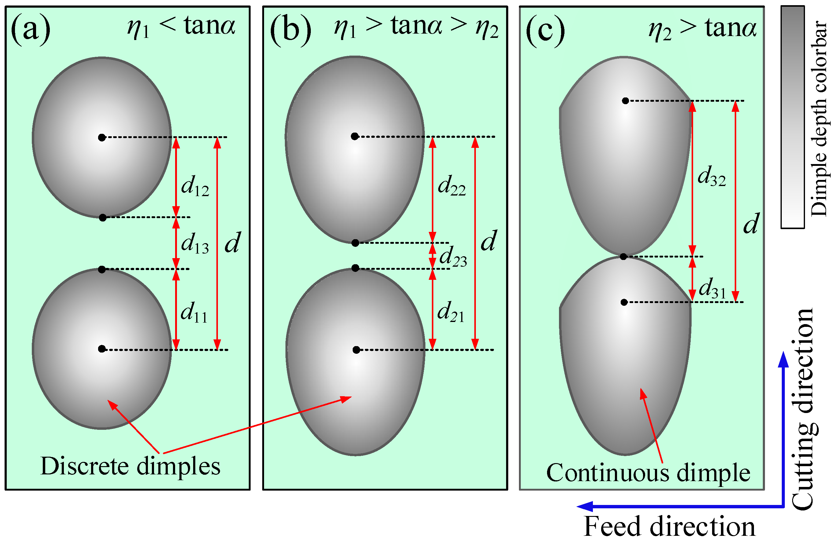
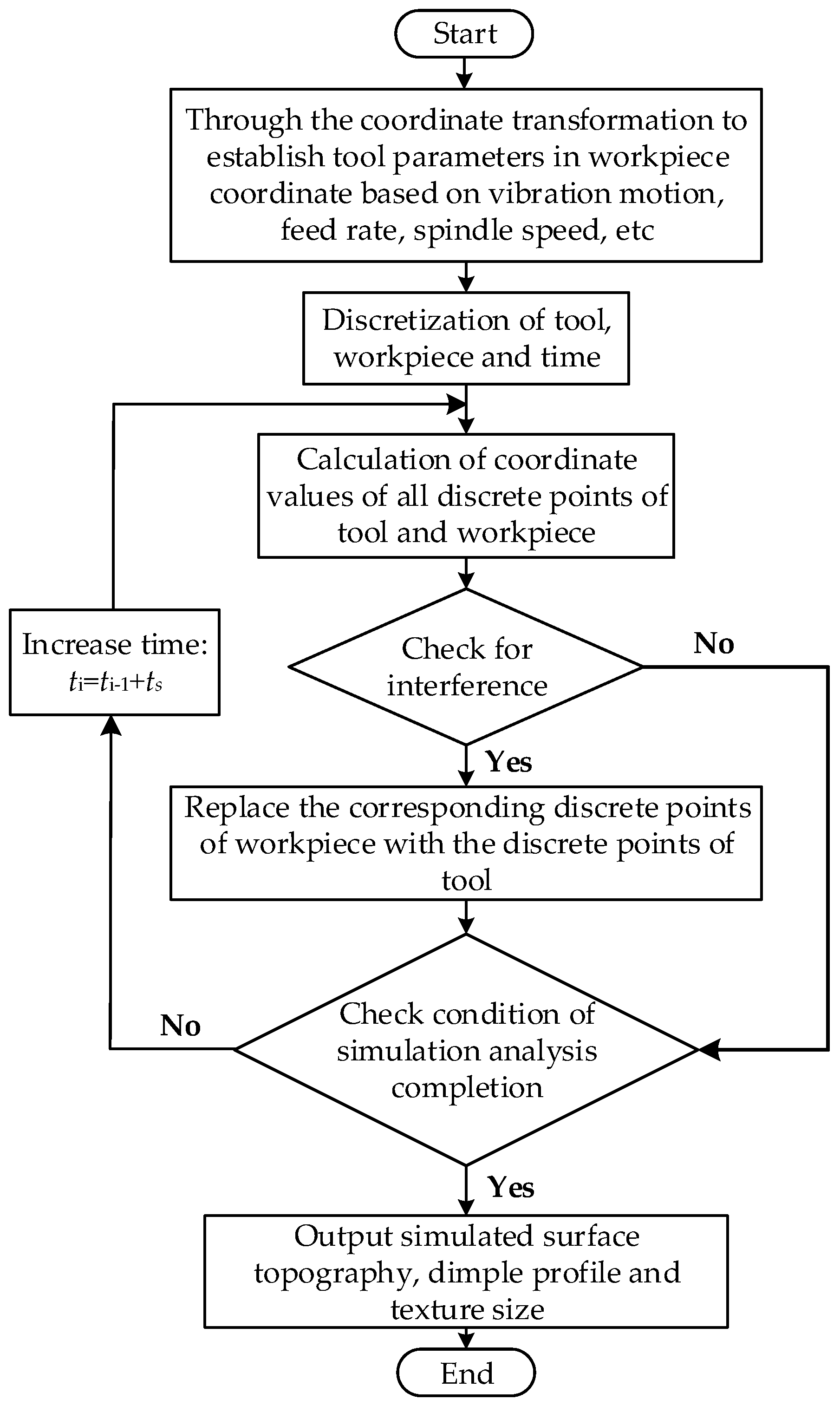
3. Simulation Analysis

3.1. Simulation Model

Simulation analysis is an effective way to predict the surface topography and provide the reference for the optimization of processing parameters. Guo et al. used a proposed simulation model to predict the texture topography of surface fabricated by elliptical vibration texturing process, and the feasibility of simulation model is verified by experiments [21,32]. On account of the proposed theoretical model, a simulation model, referring the previous model [21,32], is further modified for this 1D UVAT. The proposed simulation model is used for computational analysis, which can output the simulated topography of the micro-textured surface, dimple profile, and corresponding texture size. The principle of tool profile replication is the basis for the simulation analysis of surface topography. That is, under the ideal assumption, the texture topography is the reflection of tool edge geometry and motion path on the workpiece surface. The overall flow chart of the simulation process can be seen in Figure 10.
For the simulation analysis, it is mainly divided into four aspects, including the establishment of tool geometry model, space coordinate transformation, build of motion equation of 1D UVAT, and discretization of space and time. Same with the theoretical analysis, the simulation model is also built from the perspective of geometric kinematics. The elastic–plastic deformation of material and tool wear in the actual 1D UVAT process has not been considered. The input of processing parameters and output of 3D surface topography can be realized through establishing the algorithm programmed by MATLAB.

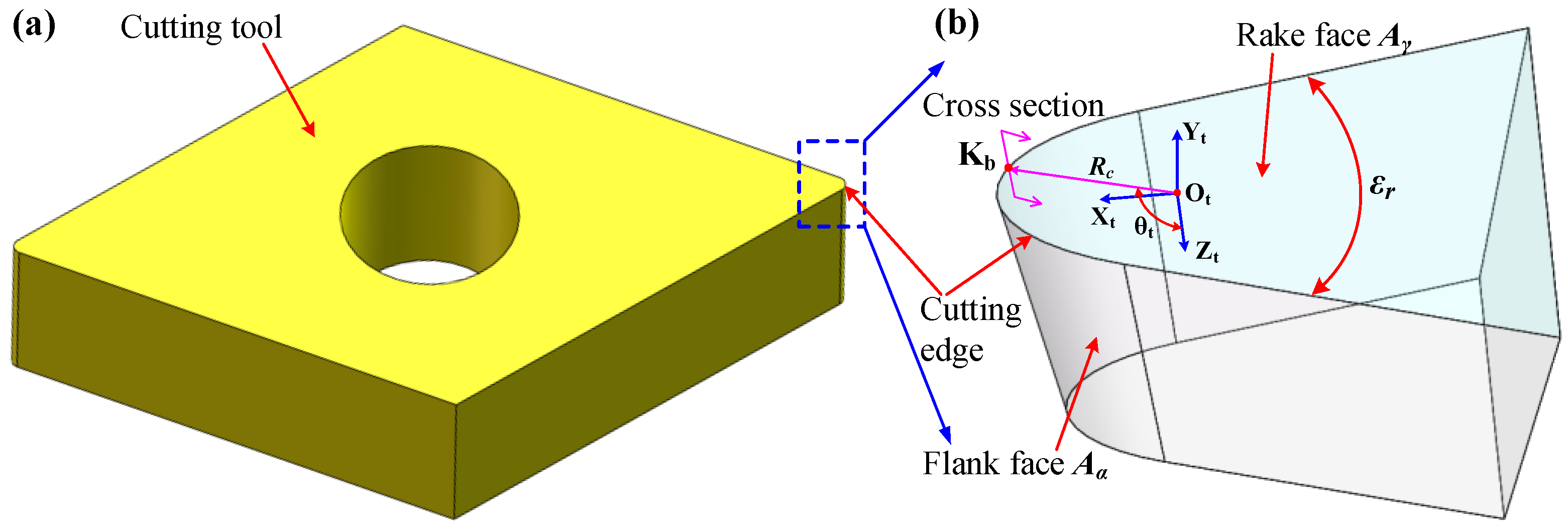
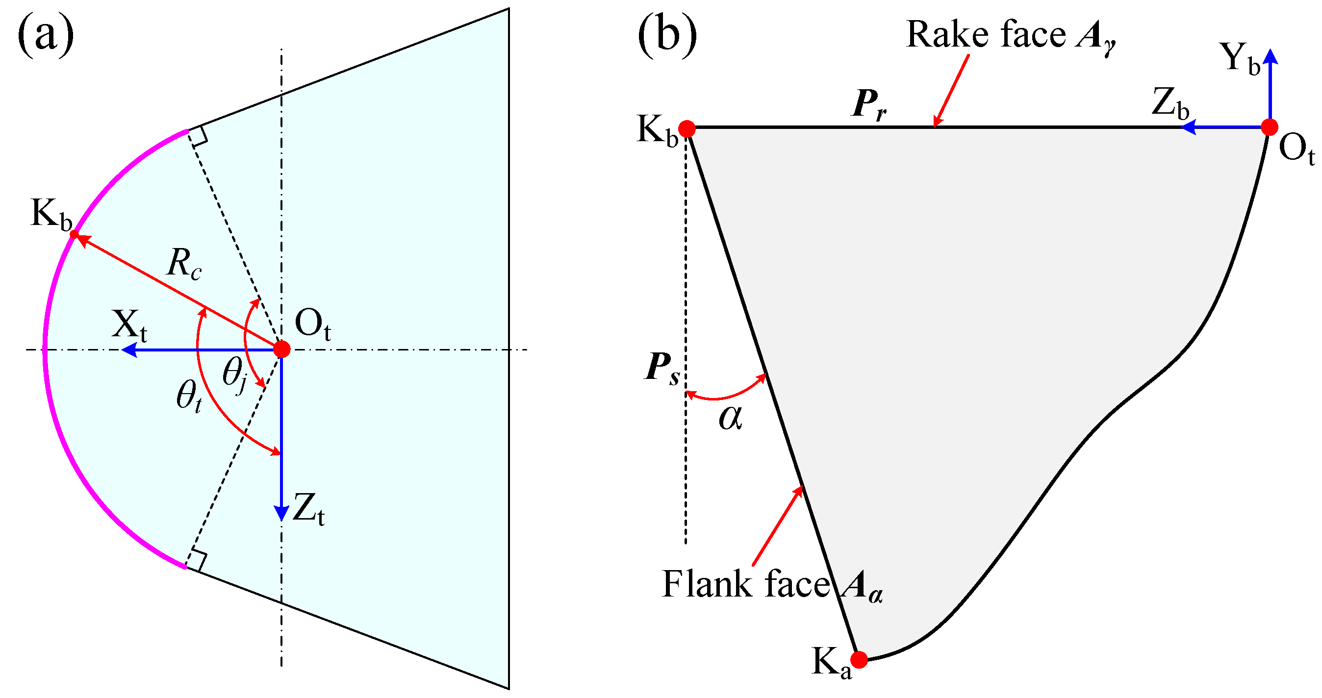
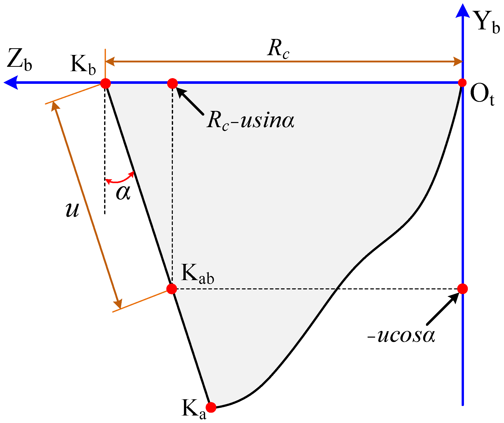
3.1.1. Tool Geometry Model

For this paper, an indexable cutting tool with symmetrical geometric shape is selected, as shown in Figure 11a. The shape of tool is prismatic. For the simulation, it only needs a part of the cutting tool, including the cutting edge, to establish the tool geometry model, as shown in Figure 11b. The angle between the main and auxiliary cutting edges is εr. As shown in Figure 11b, the tool geometric model consists of three parts, the rake face Aγ, flank face Aα, and cutting edge. It can be seen from the above theoretical analysis that the parts of the tool that mainly affects the micro-textured surface topography are the flank face and cutting edge. The depth of the cut and vibration amplitude are relatively small. Therefore, for the purpose of simplifying the modeling process of the tool and improving the simulation computational efficiency, it is only necessary to establish the cutting edge (pink line segment) and corresponding flank face, as shown in Figure 12. The angle corresponding to this cutting-edge fillet is θj. The relationship between εr and θj can be expressed as:
θ j = π ε r
It should be specially noted that, in this simulation analysis process, the selection of feed rate, based on this tool geometry, should not be greater than the value of lj (length of green line, as shown in Figure 12). The lj can be calculated by the following:
l j = 2 R c sin   θ j 2
Only under this condition, the tool geometry model, composed of cutting edge and flank face, corresponding to the included angle θj, can satisfy the reflection conditions between the cutting tool and workpiece during this surface texturing process.
Before establishing the tool geometry model, the following assumptions need to be made:
(1)
The rake face Aγ is a simple plane, and the corresponding rake angle is 0°, which is convenient to establish the geometric equation of the cutting edge and flank face.
(2)
The cutting edge is sharp, which is not rounded.
It is first to establish the tool coordinate system Ot-XtYtZt, which takes the center Ot of cutting-edge fillet as the original point, as shown in Figure 11b. Yt is perpendicular to the rake face, Zt is in the feed direction, and Xt is in the depth direction, perpendicular to Zt and Yt at the same time. Based on this coordinate system, the flank face and cutting edge can be expressed through the establishment of equations.
As shown in Figure 11 and Figure 13a, a point (Kb) is set on the cutting edge. The angle between the line OtKb and the Zt axis is θt, and its value range is [ π θ j 2 , π + θ j 2 ] . The cross-section of the cutting tool, along OtKb direction, can be seen in Figure 13b. The clearance angle (α) is the angle between flank face (Aα) and cutting plane (Ps). The rake face (Aγ) coincides with the basal plane (Pr). The coordinate axis, along the OtKb direction, is set as the Zb axis. The Yb axis coincides with the Yt axis.
The detailed expression of line KbKa in YbZb rectangular coordinates can be seen in Figure 14. Kab is the point on the line KbKa that corresponds to the profile of flank face. The distance from point Kab to vertex Kb is set to u. The coordinate values of the Kab point, corresponding to the Yb and Zb axis, are −ucosα and Rcusinα, respectively. Therefore, the profile line KbKa can be expressed by the given variable u:
X b ( u ) = 0   Y b ( u ) = u cos   α Z b ( u ) = R c u sin   α
Considering the angle θt, the equation of tool geometry in the tool coordinate system can be expressed through a vector group [Xt(u, θt), Yt(u, θt), Zt(u, θt), 1]T by the following:
X t ( u ,   θ t ) = ( R c u sin   α ) sin   θ t Y t ( u ,   θ t ) = u cos   α Z t ( u ,   θ t ) = ( R c u sin   α ) cos   θ t
When u = 0, the equation of tool geometry model expresses the cutting edge corresponding to the angle θt. When u > 0, the equation of tool geometry model expresses the flank face corresponding to the angle θt.

3.1.2. Space Coordinate Transformation

The simulation analysis needs to establish four coordinate systems to transform the expression of the geometry model from the tool coordinate systems to the workpiece coordinate systems, as shown in Figure 15. Except for the tool coordinate system Ot-XtYtZt, the other three coordinate systems are tool–machine coordinate system Ot-XtmYtmZtm, machine coordinate system Om-XmYmZm, and workpiece coordinate system Om-XwmYwmZwm. For the coordinate systems built by Guo et al. [32], three angles, including Gα, Hα, and Lα, need to be established for the rotation transformation from tool coordinate system to tool–machine coordinate system. In the paper, the parameters of Gα, Hα, and Lα are all set to 0°, which can also satisfy the processing requirements of 1D UVAT. Therefore, the established tool coordinate system coincides with the tool–machine coordinate system. The tool–machine coordinate system can be transformed to the machine coordinate system, through the matrix T (Xinit+DOC, hm, fv·t), which can be expressed by the following:
T ( X i n i t + D O C , h m , f v t ) = [ 1 0 0 X i n i t + D O C 0 1 0 h m 0 0 1 f v t 0 0 0 1 ]
where Xinit is the initial contact position of cutting tool, hm is the vertical distance from the original point Ot in tool coordinate system to the workpiece axis, and fv is the feed speed. As for the fv, it can be calculated by the following:
f v = f n
The machine coordinate system needs to use a rotation matrix RZ(−ωst) to transform into the workpiece coordinate system. The rotation matrix can be expressed as [32]:
R Z ( ω s t ) = [ cos   ω s t sin   ω s t 0 0 sin   ω s t cos   ω s t 0 0 0 0 1 0 0 0 0 1 ]
where ωs is the angular velocity of workpiece rotation. The rotation angle is 0° at initial time and increases with the time.
Through the above two transformations of the coordinate system, the tool geometry model, at any time, can be expressed in the workpiece coordinate system by the following:
[ X w k ( u , θ t , t ) Y w k ( u , θ t , t ) Z w k ( u , θ t , t )   1 ] = R Z ( ω s t ) T ( X i n i t + D O C , h m , f v t ) [ X t ( u , θ t ) Y t ( u , θ t ) Z t ( u , θ t )   1 ] = [ cos   ω s t sin   ω s t 0 0 sin   ω s t cos   ω s t 0 0 0 0 1 0 0 0 0 1 ] [ 1 0 0 X i n i t + D O C 0 1 0 h m 0 0 1 f v t 0 0 0 1 ] [ X t ( u , θ t ) Y t ( u , θ t ) Z t ( u , θ t )   1 ]

3.1.3. Motion Equation of 1D UVAT

For achieving the expression of the tool geometry model in the surface texturing process of 1D UVAT, the ultrasonic vibration equation needs to be added to the Equation (28), and the corresponding tool geometry model can be expressed as the following:
[ X w k ( u , θ t , t ) Y w k ( u , θ t , t ) Z w k ( u , θ t , t )   1 ] = R Z T { [ X t ( u , θ t ) Y t ( u , θ t ) Z t ( u , θ t )   1 ] + [ A sin   2 π f u s t 0 0 0 ] }
As for the workpiece surface, with length of L and initial radius of R0, it can be easily expressed in cylindrical coordinate system:
ρ ( L w , θ w ) = R 0
where Lw and θw are the function parameters, and the corresponding value ranges are [0, L] and [0, 2π], respectively.
In order to improve the operating efficiency of the MATLAB program, the equation of tool geometry model with ultrasonic vibration is more appropriate to be expressed in cylindrical coordinate system [21,32]. The expression can be given by the following:
[ L w k ( u , θ t , t ) ρ w k ( u , θ t , t ) θ w k ( u , θ t , t ) ] = [ Z w k ( u , θ t , t ) X w k ( u , θ t , t ) + i Y w k ( u , θ t , t ) a r g { X w k ( u , θ t , t ) + i Y w k ( u , θ t , t ) } ]

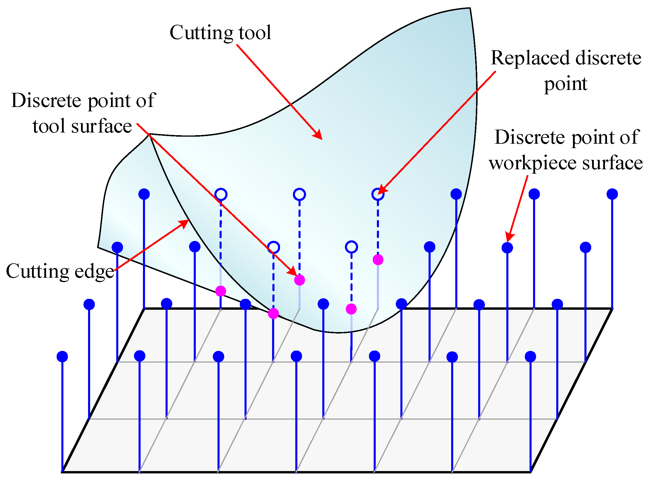
3.1.4. Discretization of Space and Time

In the programing process of MATLAB, the discretization of parameters, corresponding to space and time, should be performed. The cutting tool and workpiece both need to be discretized into mesh grids. The corresponding interval of mesh grids depends on a proposed spatial resolution (ζ), and the angle resolution is determined by the ratio of spatial resolution to the corresponding radius [21,32]. For the workpiece, the length Lw and the azimuth θw are discretized by the resolutions of ζ and ζ/R0, respectively. For the cutting tool, the parameters of u and θt are also discretized by the resolutions of ζ and ζ/Rc, respectively. The discretization of time can be achieved by setting the time step (ts). The size of time step is determined by the number of time point (nt) taken in a vibration period, and it can be expressed by the following:
t s = 1 f u s n t
In order to make the cutting trace over time smooth, the number of time point should not be too small. Figure 16 illustrates the replacement principle of discrete points between the cutting tool and workpiece surface at a certain discrete time point (ti). When tool cuts into workpiece surface, the discrete points of the tool surface (pink dots in Figure 16) are below the discrete points of the workpiece surface (blue dots in Figure 16), and then the discrete points of tool surface will replace the corresponding discrete points of the workpiece surface to form a new workpiece surface. When tool does not cut into the workpiece surface, the replacement of discrete points will not be happened. When the simulation computational process is finished, the simulated topography of the micro-textured surface can be output.
The spatial resolution and size of time step can directly affect the operating efficiency of the program and simulation precision of the surface topography. Therefore, on the premise of ensuring the operating efficiency of program, choosing a small spatial resolution and time step is helpful to improve the simulation precision of the surface topography and dimple profile. In this simulation analysis, the ζ is set to 0.2 μm and nt is set to 200.

3.2. Results and Discussion

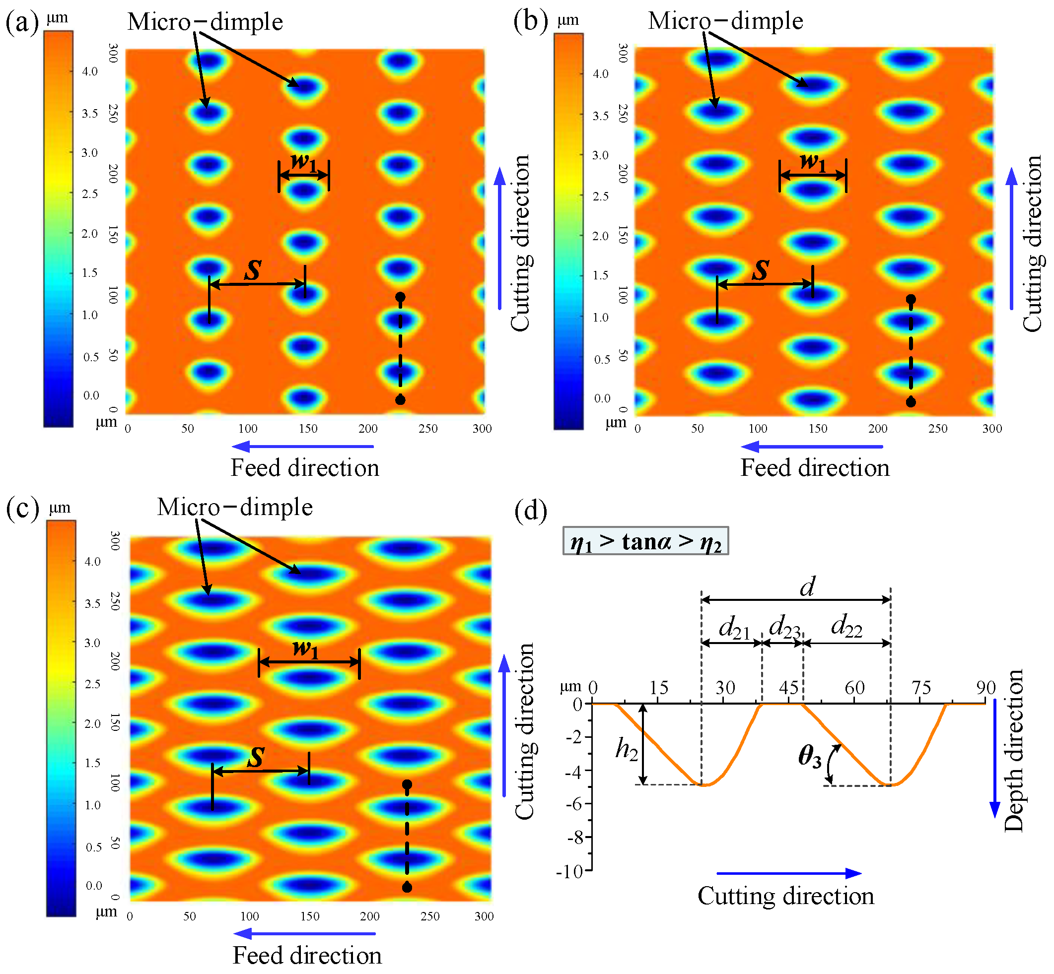
3.2.1. Clearance Angle

Referring to the previous study [28,29,30], the vibration frequency and amplitude of UVD are still chosen to be 19,670 Hz and 3.9 μm, respectively. The radius of the workpiece is 20 mm, depth of the cut is 1 μm (which is less than the vibration amplitude), spindle speed is 400 r/min, feed rate is 80 μm/rev, and nose radius of the cutting tool is 100 μm. For the cutting tool, the angle between the main and auxiliary cutting edges (εr) is 55°. Corresponding to the vibration frequency of 19,670 Hz, the size of time step is 2.5 × 10⁻⁷ s. During the simulation computational process, the parameters of fus, R, and DOC remain unchanged. When the intersecting rates of η1 and η2 remain constant, the intersection state between the flank face and cutting trace can be changed by choosing different clearance angles. Therefore, in order to confirm the effect of the clearance angle on the fabrication of the micro-textured surface, three clearance angles should be chosen to meet the requirements of three intersection states. For determining the values of η1 and η2, corresponding to the above processing parameters, the values of d and t1 can be firstly figured out. According to the Equations (2) and (9), the calculated values of d and t1 are 43 μm and 1.48 × 10⁻⁵ s, respectively. Then, the value of d1 is calculated to be 12 μm, according to Equation (10). According to the Equation (4), the intersecting rate of η1 can be calculated by the following:
η 1 = tan   θ 1 = D O C + A d 2 = 0.4
The corresponding angle θ1 can be obtained by the following:
θ 1 = a r c tan   ( η 1 ) = 21.8 °
According to Equation (5), the intersecting rate of η2 can be obtained by the following calculation:
η 2 = tan   θ 2 = D O C + A d d 1 = 0.16
The corresponding angle θ2 can be obtained by the following:
θ 2 = a r c tan   ( η 2 ) = 9.1 °
Consequently, for the purpose of achieving the three intersection states between flank face and cutting trace, the chosen clearance angles used in the simulation analysis are 25°, 15°, and 5°, respectively. The corresponding variation of surface topography and dimple profile can be seen in Figure 17. The output range of surface topography is selected to be 300 μm × 300 μm. Because ζ is set to 0.2 μm, the minimum distance between the adjacent discrete points on the Y and Z axes is 0.2 μm. The length of the dimple profile along the Y axis is 90 μm, which consists of 450 discrete points. As for the X axis, the reference plane, which corresponds to the uncut surface, is set at 0 μm, and the texture depth is shown in the negative axis.
When the clearance angle is 25°, there is no intersection between the flank face and cutting trace (η1 < tan α). The corresponding surface topography and dimple profile can be seen in Figure 17a,b. It can be seen that the discrete, oval-like micro-dimples are evenly distributed on the workpiece surface, which is consistent with the dimple shape shown in Figure 9a. The areas between adjacent dimples refer to the uncut surfaces. The distance between the adjacent dimples, along feed direction, S, is equal to the feed rate, which is measured to be 80 μm. The simulated dimple profile, in the cutting direction, is also consistent with the theoretical dimple profile shown in Figure 5b. The distance (d) also includes three parts, i.e., d11, d13, and d12. The corresponding simulated values of d11, d13, and d12 are 13.2, 16.4, and 13.2 μm, respectively. Compared with the theoretical values of 12.4, 17.8, and 12.4 μm, the deviations are 6.5%, 7.9%, and 6.5%, respectively. As for the dimple depth h1, the simulated value is same as the theoretical value, i.e., 4.9 μm. The corresponding comparative values of the dimple profile are summarized in Table 1. Through the above analysis, the simulation results, regarding the size, shape, and distribution of the micro-dimples generated under an intersection state of η1 < tan α, are highly consistent with the theoretical analysis.
When the clearance angle is 15°, the flank face intersects with the cutting trace, and the corresponding intersection state is η1 > tan α > η2. The simulated surface topography and dimple profile can be seen in Figure 17c,d. The discrete dimples are also evenly distributed on the workpiece surface. Same with the theoretical analysis, under this intersection state, the oval-like dimple is asymmetric along cutting direction, as shown in Figure 17c. The simulated dimple profile is also consistent with the theoretical dimple profile shown in Figure 6b. The distance (d) also includes three parts, i.e., d21, d23, and d22. The angle θ3, corresponding to d22, also exists in the dimple profile, as shown in Figure 17d. The simulated values of d21, d23, and d22 are 12.6, 10.6, and 19.6 μm, respectively. Compared with the theoretical values of 12.4, 11.9 and 18.3 μm, the deviation is 1.6%, 10.9%, and 7.1%, respectively. As for the dimple depth, h2, the simulated value is consistent with the theoretical value, which are both 4.9 μm. The simulated value of θ3 is 14.0°, which has a deviation of 6.7%, compared with the clearance angle. The corresponding comparative values of the dimple profile are summarized in Table 1. In summary, the influence of the intersection state (η1 > tan α > η2) on the surface topography and dimple profile can be further verified from the respective simulation analysis.
When the clearance angle is 5°, the flank face intersects with the cutting trace, and the corresponding intersection state is η2 > tan α. The simulated surface topography and dimple profile can be seen in Figure 17e,f. It can be seen that the micro-dimples in the cutting direction change from discrete to continuous. The micro-dimples in the feed direction continue to be discrete, and the middle area between the adjacent dimples also refers to the uncut surface. Same with the dimple shape illustrated in Figure 9c, the simulated dimple shape is also scaly-like, as shown in Figure 17e. Under this intersection state, the simulated dimple profile is consistent with the theoretical dimple profile, shown in Figure 7b. The distance (d) also includes two parts, i.e., d31 and d3. The angle θ3 corresponding to d32 also exists in the dimple profile, as shown in Figure 17f. The simulated values of d31 and d32 are 9.4 and 33.2 μm, respectively. Compared with the theoretical values of 9.0 and 33.6 μm, the deviation is 4.4% and 1.2%, respectively. As for the dimple depth h3, the simulated value is consistent with the theoretical value, which are both 2.9 μm. Same with the value of clearance angle, the simulated value of θ3 is also 5°. The corresponding comparative values of the dimple profile are summarized in Table 1. When the intersection state is η2 > tan α, the change rule of surface topography and dimple profile is also verified by the simulation analysis.
The simulation results show that, when other processing parameters remain unchanged (that is, the cutting trace remains unchanged), the discrete or continuous micro-dimples, with different sizes and specific shapes, can be generated on cylindrical surface by changing the clearance angle.

3.2.2. Spindle Speed

According to theoretical analysis, the cutting trace can be changed by choosing a different spindle speed. Therefore, when the clearance angle and other processing parameters remain unchanged, the intersection state between the flank face and cutting trace will also change as the spindle speed changes. In order to choose the proper value of spindle speed, two critical spindle speeds of n1 and n2 need to be firstly determined. When flank face intersects with the cutting trace on point J (where the angle θ1 is equal to the clearance angle), the critical spindle speed is defined as n1. When flank face intersects with the cutting trace on point K (where the angle θ2 is equal to the clearance angle), the critical spindle speed is defined as n2. When clearance angle is 15° and other processing paremeters (fus, A, R, DOC, f, and Rc) keep unchanged, n1 can be calculated to be 590 r/min, according to the Equations (4) and (8)–(10), and n2 can be calculated to be 243 r/min, according to the Equations (2), (5) and (8)–(10).
On account of the critical spindle speeds of n1 and n2, the spindle speeds of 800, 400, and 100 r/min are chosen for the simulation analysis, which can achieve the intersection states of η1 < tan α, η1 > tan α > η2 and η2 > tan α, respectively. The corresponding variation of the surface topography and dimple profile, under different spindle speeds, can be seen in Figure 18.
When the spindle speed is 400 r/min, the intersection state between the flank face and cutting trace is η1 > tan α > η2; the corresponding simulated surface topography and dimple profile are shown in Figure 18c,d, which are same as Figure 17c,d. The relevant content has been discussed above in Section 3.2.1. Except for the spindle speed, when the following processing parameters, including vibration amplitude, nose radius, and feed rate, are discussed, Figure 17c,d is still chosen as the specified surface topography and dimple profile, simulated under η1 > tan α > η2. Therefore, in order to better show the difference of the surface topography and dimple profile, concerning different processing parameters, Figure 17c,d is still added as Figure 19c,d, Figure 20b,d, and Figure 21b,d to the following figures, respectively.
When the spindle speed is 800 r/min, the corresponding intersection state is η1 < tan α, and the simulated surface topography and dimple profile can be seen in Figure 18a,b. With spindle speed increasing from 400 to 800 r/min, the flank face has no intersection with the cutting trace, and the distance between adjacent dimples, along cutting direction, also increases. The distribution of micro-dimples becomes sparser on the workpiece surface. The dimple shape becomes oval-like, with symmetry characteristics. The simulated dimple profile is also consistent with that in Figure 5b, and the distance (d) between adjacent dimples also includes three parts, i.e., d11, d13, and d12. The corresponding simulated values of d11, d13, and d12 are 24.6, 35.9, and 24.6 μm, respectively. Compared with the theoretical values of 24.8, 35.6, and 24.8 μm, the deviation is 0.8%, 0.8%, and 0.8%, respectively. As for the dimple depth, h1, the simulated value is same as the theoretical value, which are both 4.9 μm. The corresponding comparative values of dimple profile are summarized in Table 2.
When the spindle speed changes to 200 r/min, the intersection state is η2 > tan α, and the corresponding simulated surface topography and dimple profile can be seen in Figure 18e,f. It can be found that, with the spindle speed decreasing from 400 to 200 r/min, the intersection state between the flank face and cutting trace has changed, and the distribution characteristic of the adjacent dimples, in the cutting direction, changes from discrete to continuous. The distance (d) is then reduced from 42.6 to 21.3 μm. The corresponding simulated values of d31 and d32 are 5.8 and 15.6 μm, respectively. Compared with the theoretical values of 5.6 and 15.7 μm, the deviation is 3.6% and 0.6%, respectively. As for the dimple depth, h3, the simulated value is 4.1 μm, which has a deviation of 2.4%, compared with the theoretical value of 4.2 μm. The angle θ3 is simulated to be 14.7°, which has a deviation of 2.0%, compared with the clearance angle. The corresponding comparative values of the dimple profile are also summarized in Table 2.
The simulation results show that, when the clearance angle remains unchanged (i.e., the flank face remains unchanged), the intersection state between the flank face and cutting trace can also be changed by choosing different spindle speed, and then the discrete or continuous micro-dimples, with different sizes and specific shapes, can be generated on the cylinderical surface. In addition, the distance between adjacent dimples along the cutting direction, as well as the distribution density of the dimple, also vary with the change of spindle speed.

3.2.3. Vibration Amplitude

Based on the theoretical analysis, the cutting trace can also be changed by choosing different vibration amplitude. Therefore, when the clearance angle and other processing parameters remain unchanged, the intersection state between the flank face and cutting trace will also vary with the vibration amplitude. In order to choose the proper simulated value of vibration amplitude, two critical vibration amplitudes, A1 and A2, need to be firstly determined. When flank face intersects with cutting trace on point J (where the angle θ1 is equal to clearance angle), the critical vibration amplitude is defined as A1. When flank face intersects with cutting trace on point K (where the angle θ2 is equal to clearance angle), the critical vibration amplitude is defined as A2. When clearance angle is 15°, the spindle speed is 400 r/min, and other processing paremeters (fus, R, DOC, f, and Rc) keep unchanged; A1 can be calculated to be 2.6 μm, according to Equations (4) and (8)–(10), and A2 can be calculated to be 7.3 μm, according to Equations (2), (5) and (8)–(10).
In view of the critical vibration amplitudes of A1 and A2, the vibration amplitudes of 2.0, 3.9, and 8.0 μm are chosen for the simulation analysis, which can achieve the intersection states of η1 < tan α, η1 > tan α > η2 and η2 > tan α, respectively. The corresponding variation of surface topography and dimple profile, under different vibration amplitudes, can be seen in Figure 19. When the vibration amplitude is 3.9 μm, the intersection state is η1 > tan α > η2, and the corresponding simulated surface topography and dimple profile are shown in Figure 19c,d, which are same as in Figure 17c,d. The relevant content has been discussed above in Section 3.2.1.
When the vibration amplitude is 2.0 μm, the simulated surface topography and dimple profile can be seen in Figure 19a,b. With the vibration amplitude increasing from 3.9 to 2.0 μm, the flank face has no intersection with the cutting trace. The dimple shape also becomes oval-like, with symmetry characteristics. The distance (d) between adjacent dimples also includes three parts of d11, d13 and d12. The corresponding simulated values of d11, d13 and d12 are 14.2, 14.0, and 14.4 μm, respectively. Compared with the theoretical values of 14.2, 14.2, and 14.2 μm, the deviation is 0%, 1.4%, and 1.4%, respectively. As for the dimple depth, h1, the simulated value is same with the theoretical value, which are both 3 μm. The corresponding comparative values of the dimple profiles are summarized in Table 3. Same with the theoretical analysis, when the vibration amplitude changes from 3.9 to 2.0 μm, the dimple width (w1) also decreases from 61.8 to 48.6 μm.
When the vibration amplitude is 8.0 μm, the intersection state is η2 > tan α, and the corresponding simulated surface topography and dimple profile can be seen in Figure 19e,f. It can be found that the distribution of adjacent dimples, in the cutting direction, changes from discrete to continuous. The corresponding simulated values of d31 and d32 are 11.2 and 31.4 μm, respectively. Compared with the theoretical values of 11.0 and 31.6 μm, the deviation is 1.8% and 0.6%, respectively. As for the dimple depth, h3, the simulated value is 8.3 μm, which has a deviation of 2.4%, compared with the theoretical value of 8.5 μm. The angle θ3 is simulated to be 14.7°, which has a deviation of 2.0%, compared with the clearance angle. The corresponding comparative values of dimple profile are also summarized in Table 3. Same with the theoretical analysis, when vibration amplitude changes from 3.9 to 8.0 μm, the dimple width also increases from 61.8 to 82.9 μm.
The simulation results show that, when clearance angle remains unchanged, the intersection state can also be changed by choosing different vibration amplitude, and then the coresponding discrete or continuous micro-dimples, with different sizes and specific shapes, can also be fabricated on the cylindrical surface.

3.2.4. Nose Radius

The nose radiuses chosen for the simulation analysis are 50, 100, and 200 μm. Other processing parameters are the same as those used in Figure 17c,d. When the nose radius changes from 50, 100, to 200 μm, the corresponding simulated surface topographies and dimple profiles can be seen in Figure 20. It can be found that the dimple profiles associated with a different nose radius are all the same, as shown in Figure 20d. The only thing that has changed is the dimple width. Compared with Figure 20b, when nose radius is 50 μm, the dimple width is reduced to 43.2 μm, and the corresponding simulated surface topography is shown in Figure 20a. Compared with Figure 20b, when nose radius becomes 200 μm, the dimple width is increased to 88.0 μm, and the corresponding simulated surface topography is shown in Figure 20c. From the simulation analysis, the dimple width increases with the increase of nose radius.

3.2.5. Feed Rate

The feed rates chosen for the simulation analysis are 40, 80, and 120 μm/rev. Other processing parameters are the same as those used in Figure 17c,d. When feed rate changes from 40, 80, and 120 μm/rev, the corresponding simulated surface topographies and dimple profiles can be seen in Figure 21. Same with Figure 20d, the dimple profiles under different feed rates also keep consistent, as shown in Figure 21d. It can be seen from Figure 21a–c that the distance between adjacent dimples, along feed direction, which is equal to the feed rate, is also increased from 40, 80, and 120 μm. The distribution density of the micro-dimples in the feed direction on the surface also varies with the change of the feed rate. It is further confirmed that the feed rate has great effect on the distance between adjacent dimples along the feed direction.

4. Conclusions

Based on the results and analysis in the present paper, the following conclusions can be drawn.
(1)
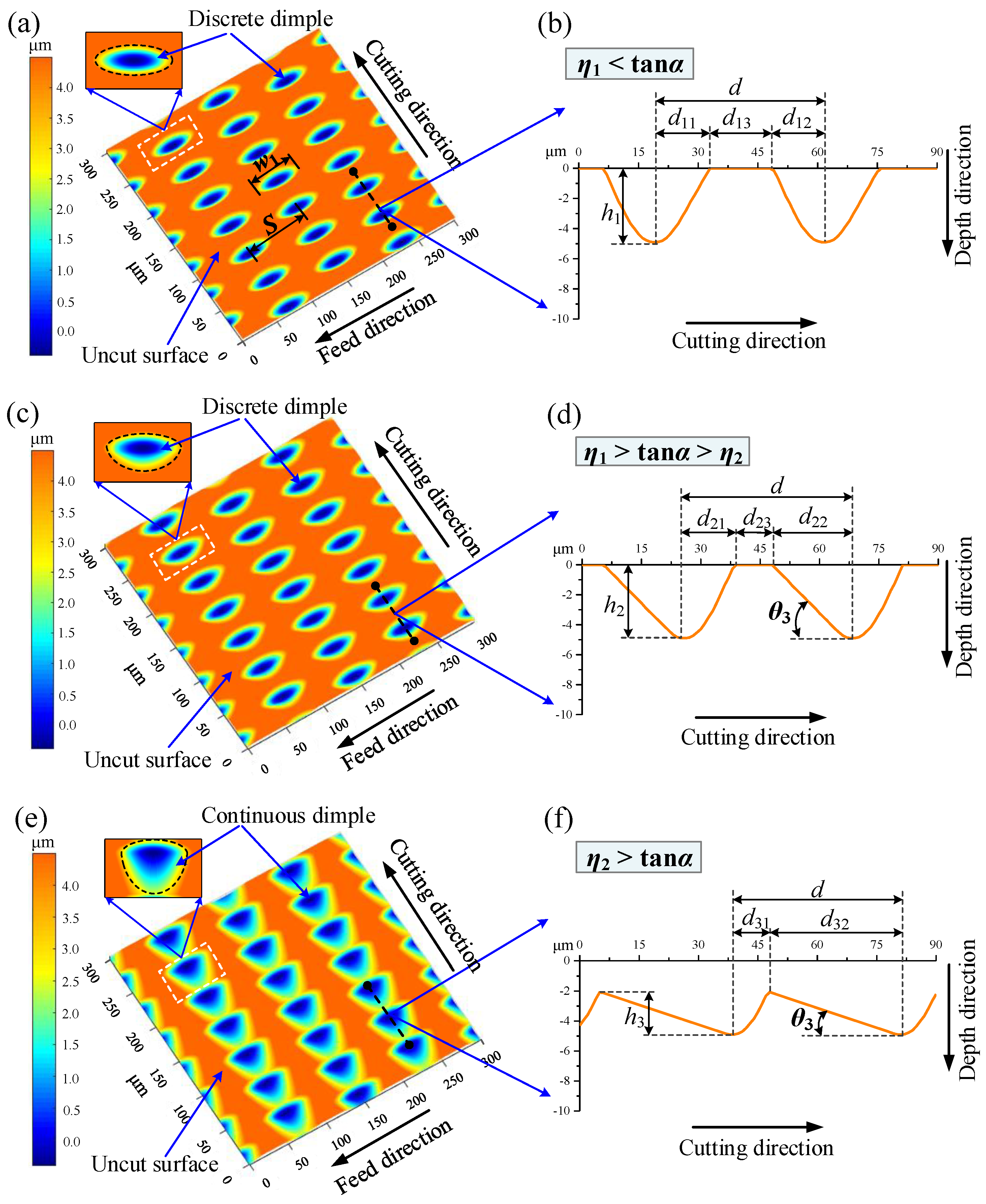
From the perspective of geometric kinematics, the proposed theoretical model of this 1D UVAT can detailedly illustrate the generation mechanism and dimple characteristics of micro-textured surfaces, fabricated under intermittent cutting conditions, which can also effectively provide the quantitative analysis for the textured parameters. The intersection states between flank face and cutting trace, including η1 < tan α, η1 > tan α > η2, and η2 > tan α, are the key factors to influence the distribution, size, and shape of the micro-dimples. Certainly, the theoretical model does not consider the factors including the elastic–plastic deformation of the workpiece material, which probably exists in the actual cutting process.
(2)
The simulation results not only confirm the proposed theoretical model, but also prove that the established simulation model is effective in predicting the characteristics of the surface topography and dimple profile. Through comparing the simulated and theoretical values of the dimple profiles, fabricated under different processing parameters, it can be found that the maximum deviation can reach 10.9%, and the minimum deviation can reach 0%. In order to further improve the accuracy of the simulation analysis, more reasonable spatial resolutions and time steps should be selected.
(3)
By choosing different clearance angles, spindle speeds, or vibration amplitudes, the intersection state between flank face and cutting trace can be changed, and then the corresponding discrete or continuous micro-dimples, with different sizes and specific shapes, can be generated on the cylinderical surface. In addition to this, the spindle speed and vibration amplitude have influence on the distribution density of the dimple in the cutting direction and dimple width, respectively. Although the nose radius and feed rate have no effect on the intersection state between the flank face and cutting trace, they can directly influence the dimple width and distance between adjacent dimples along the feed direction, respectively.
(4)
Under the intermittent cutting condition, the proposed surface texturing method of 1D UVAT is proved to be a feasible and simple processing way to fabricate micro-textured surfaces. The corresponding theoretical and simulation analysis in the paper also lay a valuable foundation for the further optimization of the processing parameters and experimental fabrication of micro-textured surfaces.
(5)
As for further development, additional studies need to be performed in the future. Further optimization of the mathematical formulation, which can consider factors including elastic–plastic deformation, should be carried out. Corresponding experimental tests should be performed to verify the accuracy of the theoretical and simulation results and obtain the corresponding actual image of the micro-textured surface. Because the tool wear, existing in the actual texturing process, may also affect the generation of surface texture topography, the corresponding study should also be carried out through experimental tests.

Author Contributions

Conceptualization, X.L. and J.Z.; methodology, X.L.; software, X.L.; validation, X.L. and W.H.; formal analysis, X.L.; investigation, X.L.; resources, J.Z.; data curation, X.L.; writing—original draft preparation, X.L.; writing—review and editing, L.L. and W.H.; visualization, L.L.; supervision, J.Z.; project administration, J.Z.; funding acquisition, J.Z. All authors have read and agreed to the published version of the manuscript.

Funding

This research was funded by the National Natural Science Foundation of China, grant number 51475275.

Data Availability Statement

Not Applicable.

Acknowledgments

The authors would like to thank Tingrui Liu for the simulation analysis.

Conflicts of Interest

The authors declare no conflict of interest. The funders had no role in the design of the study; in the collection, analyses, or interpretation of data; in the writing of the manuscript, or in the decision to publish the results.

References

  1. Bruzzone, A.A.G.; Costa, H.L.; Lonardo, P.M.; Lucca, D.A. Advances in engineered surfaces for functional performance. CIRP Ann. 2008, 57, 750–769. [Google Scholar] [CrossRef]
  2. Gropper, D.; Wang, L.; Harvey, T.J. Hydrodynamic lubrication of textured surfaces: A review of modeling techniques and key findings. Tribol. Int. 2016, 94, 509–529. [Google Scholar] [CrossRef] [Green Version]
  3. Lu, P.; Wood, R.J.K. Tribological performance of surface texturing in mechanical applications—A review. Surf. Topogr. Metrol. 2020, 8, 043001. [Google Scholar] [CrossRef]
  4. Sudeep, U.; Tandon, N.; Pandey, R.K. Performance of lubricated rolling/sliding concentrated contacts with surface textures: A review. J. Tribol. 2015, 137, 031501. [Google Scholar] [CrossRef]
  5. Adjemout, M.; Brunetiere, N.; Bouyer, J. Numerical analysis of the texture effect on the hydrodynamic performance of a mechanical seal. Surf. Topogr. Metrol. 2016, 4, 014002. [Google Scholar] [CrossRef]
  6. Nitin, S.; Rajeev, V.; Sumit, S.; Saurabh, K. Qualitative potentials of surface textures and coatings in the performance of fluid-film bearings: A critical review. Surf. Topogr. Metrol. 2021, 9, 013002. [Google Scholar]
  7. Lu, X.; Khonsari, M.M. An experimental investigation of dimple effect on the stribeck curve of journal bearings. Tribol. Lett. 2007, 27, 169–176. [Google Scholar] [CrossRef]
  8. Ahmed, A.; Masjuki, H.H.; Varman, M.; Kalam, M.A.; Habibullah, M.; Al Mahmud, K.A.H. An overview of geometrical parameters of surface texturing for piston/cylinder assembly and mechanical seals. Meccanica 2016, 51, 9–23. [Google Scholar] [CrossRef]
  9. Xiong, D.; Qin, Y.; Li, J.; Wan, Y.; Tyagi, R. Tribological properties of PTFE/laser surface textured stainless steel under starved oil lubrication. Tribol. Int. 2015, 82, 305–310. [Google Scholar] [CrossRef]
  10. Saeidi, F.; Meylan, B.; Hoffmann, P.; Wasmer, K. Effect of surface texturing on cast iron reciprocating against steel under starved lubrication conditions: A parametric study. Wear 2016, 348–349, 17–26. [Google Scholar] [CrossRef] [Green Version]
  11. Varenberg, M.; Halperin, G.; Etsion, I. Different aspects of the role of wear debris in fretting wear. Wear 2002, 252, 902–910. [Google Scholar] [CrossRef]
  12. Yamakiri, H.; Sasaki, S.; Kurita, T.; Kasashima, N. Effects of laser surface texturing on friction behavior of silicon nitride under lubrication with water. Tribol. Int. 2011, 44, 579–584. [Google Scholar] [CrossRef]
  13. Wan, Y.; Xiong, D. The effect of laser surface texturing on frictional performance of face seal. J. Mater. Process. Technol. 2008, 197, 96–100. [Google Scholar] [CrossRef]
  14. Kovalchenko, A.; Ajayi, O.; Erdemir, A.; Fenske, G.; Etsion, I. The effect of laser surface texturing on transitions in lubrication regimes during unidirectional sliding contact. Tribol. Int. 2005, 38, 219–225. [Google Scholar] [CrossRef]
  15. Patel, D.S.; Singh, A.; Balani, K.; Ramkumar, J. Topographical effects of laser surface texturing on various time-dependent wetting regimes in Ti6Al4V. Surf. Coat. Technol. 2018, 349, 816–829. [Google Scholar] [CrossRef]
  16. Malek, C.K.; Saile, V. Applications of LIGA technology to precision manufacturing of high-aspect-ratio micro-components and -systems: A review. Microelectron. J. 2004, 35, 131–143. [Google Scholar] [CrossRef]
  17. Pettersson, U.; Jacobson, S. Influence of surface texture on boundary lubricated sliding contacts. Tribol. Int. 2003, 36, 857–864. [Google Scholar] [CrossRef]
  18. Zhou, R.; Cao, J.; Wang, Q.J.; Meng, F.; Zimowski, K.; Xia, Z.C. Technology effect of EDT surface texturing on tribological behavior of aluminum sheet. J. Mater. Process. Technol. 2011, 211, 1643–1649. [Google Scholar] [CrossRef]
  19. Wakuda, M.; Yamauchi, Y.; Kanzaki, S.; Yasuda, Y. Effect of surface texturing on friction reduction between ceramic and steel materials under lubricated sliding contact. Wear 2003, 254, 356–363. [Google Scholar] [CrossRef]
  20. Akhtar, R.R.; Yi, Q. A review on micro-manufacturing, micro-forming and their key issues. Procedia Eng. 2013, 53, 665–672. [Google Scholar]
  21. Guo, P. Development of the Elliptical Vibration Texturing Process; Northwestern University: Evanston, IL, USA, 2014. [Google Scholar]
  22. Moriwaki, T.; Shamoto, E. Ultraprecision diamond turning of stainless steel by applying ultrasonic vibration. CIRP Ann. Manuf. Technol. 1991, 40, 559–562. [Google Scholar] [CrossRef]
  23. Kumabe, J.; Fuchizawa, K.; Soutome, T.; Nishimoto, Y. Ultrasonic superposition vibration cutting of ceramics. J. Int. Soc. Precis. Eng. Nanotechnol. 1989, 11, 71–77. [Google Scholar] [CrossRef]
  24. Zhou, M.; Wang, X.J.; Ngoi, B.K.A.; Gan, J.G.K. Brittle-ductile transition in the diamond cutting of glasses with the aid of ultrasonic vibration. J. Mater. Process. Technol. 2002, 121, 243–251. [Google Scholar] [CrossRef]
  25. Zhou, M.; Eow, Y.T.; Ngoi, B.K.; Lim, E.N. Vibration-assisted precision machining of steel with PCD tools. Mater. Manuf. Process. 2003, 18, 825–834. [Google Scholar] [CrossRef]
  26. Zhang, J.; Cui, T.; Ge, C.; Sui, Y.; Yang, H. Review of micro/nano machining by utilizing elliptical vibration cutting. Int. J. Mach. Tools Manuf. 2016, 106, 109–126. [Google Scholar] [CrossRef]
  27. Yang, Z.; Zhu, L.; Zhang, G.; Ni, C.; Lin, B. Review of ultrasonic vibration-assisted machining in advanced materials. Int. J. Mach. Tools Manuf. 2020, 156, 103594. [Google Scholar] [CrossRef]
  28. Liu, X.; Wu, D.; Zhang, J.; Hu, X.; Cui, P. Analysis of surface texturing in radial ultrasonic vibration-assisted turning. J. Mater. Process. Technol. 2019, 267, 186–195. [Google Scholar] [CrossRef]
  29. Liu, X.; Zhang, J.; Hu, X.; Wu, D. Influence of tool material and geometry on micro-textured surface in radial ultrasonic vibration-assisted turning. Int. J. Mech. Sci. 2019, 152, 545–557. [Google Scholar] [CrossRef]
  30. Liu, X.; Hu, X.; Zhang, J.; Wu, D. Study on the fabrication of micro-textured end face in one-dimensional ultrasonic vibration-assisted turning. Int. J. Adv. Manuf. Technol. 2019, 105, 2599–2613. [Google Scholar] [CrossRef]
  31. Zhang, R.; Steinert, P.; Schubert, A. Microstructuring of surfaces by two-stage vibration assisted turning. Procedia CIRP 2014, 14, 136–141. [Google Scholar] [CrossRef]
  32. Guo, P.; Ehmann, K.F. An analysis of the surface generation mechanics of the elliptical vibration texturing process. Int. J. Mach. Tools Manuf. 2013, 64, 85–95. [Google Scholar] [CrossRef]
Figure 1. Illustration of surface texturing of 1D UVAT: (a) the overall assembly drawing of equipment for 1D UVAT; (b) principle of the texturing process; (c) continuous cutting condition (DOC > A); (d) intermittent cutting condition (DOC < A).
Machines 10 00166 g001
Figure 2. Illustration of micro-textured surface, generated under intermittent cutting conditions: (a) arrangement and geometry of micro-dimples; (b) the cross-sectional dimple profile along the feed direction.
Machines 10 00166 g002
Figure 3. Cutting trace under intermittent cutting condition.
Machines 10 00166 g003
Figure 4. Sinusoidal cutting trace varying with time.
Machines 10 00166 g004
Figure 5. Flank face has no intersection with cutting trace (η1 < tan α): (a) cutting trace; (b) cross-sectional profile of dimples.
Machines 10 00166 g005
Figure 6. Flank face intersects with the KJ segment of the cutting trace on point O (η1 > tan α > η2): (a) cutting trace; (b) cross-sectional profile of dimples.
Machines 10 00166 g006
Figure 7. The flank face intersects with the BK segment of cutting trace on point O (η2 > tan α): (a) cutting trace; (b) cross-sectional profile of dimples.
Machines 10 00166 g007
Figure 8. Sinusoidal cutting trace, varying with time, under the state of η2 > tan α.
Machines 10 00166 g008
Figure 9. Illustration of dimple shape under different states. (a) η1 < tan α; (b) η1 > tan α > η2; (c) η2 > tan α.
Machines 10 00166 g009
Figure 10. Flow chart of the simulation process.
Machines 10 00166 g010
Figure 11. Illustration of the tool geometry model: (a) the whole cutting tool; (b) the tool geometry model to be established.
Machines 10 00166 g011
Figure 12. Illustration of the selection of critical feed rate (f = lj).
Machines 10 00166 g012
Figure 13. Illustration of tool geometry on two planes: (a) XtZt plane; (b) YbZb plane.
Machines 10 00166 g013
Figure 14. The detailed expression of line KbKa in YbZb rectangular coordinates.
Machines 10 00166 g014
Figure 15. Illustration of the space coordinate transformation.
Machines 10 00166 g015
Figure 16. Replacement principle of discrete points between the cutting tool and workpiece surface.
Machines 10 00166 g016
Figure 17. Simulated surface topographies and dimple profiles under processing parameters of fus = 19,670 Hz, A = 3.9 μm, R = 20 mm, DOC = 1 μm, n = 400 r/min, f = 80 μm/rev, and Rc = 100 μm; (a,b) α = 25°; (c,d) α = 15°; (e,f) α = 5°.
Machines 10 00166 g017
Figure 18. Simulated surface topographies and dimple profiles under processing parameters of fus = 19,670 Hz, A = 3.9 μm, R = 20 mm, DOC = 1 μm, f = 80 μm/rev, α = 15°, Rc = 100 μm. (a,b) n = 800 r/min; (c,d) n = 400 r/min; (e,f) n = 200 r/min.
Machines 10 00166 g018
Figure 19. Simulated surface topographies and dimple profiles under processing parameters of fus = 19,670 Hz, R = 20 mm, DOC = 1 μm, n = 400 r/min, f = 80 μm/rev, α = 15°, Rc = 100 μm. (a,b) A = 2.0 μm; (c,d) A = 3.9 μm; (e,f) A = 8.0 μm.
Machines 10 00166 g019
Figure 20. Simulated surface topographies and dimple profiles under processing parameters of fus = 19,670 Hz, A = 3.9 μm, R = 20 mm, DOC = 1 μm, n = 400 r/min, f = 80 μm/rev, α = 15°. (a) Rc = 50 μm; (b) Rc = 100 μm; (c) Rc = 200 μm; (d) Rc = 50, 100, and 200 μm.
Machines 10 00166 g020
Figure 21. Simulated surface topographies and dimple profile under processing parameters of fus = 19,670 Hz, A = 3.9 μm, R = 20 mm, DOC = 1 μm, n = 400 r/min, α = 15°, Rc = 100 μm. (a) f = 40 μm/rev; (b) f = 80 μm/rev; (c) f = 120 μm/rev; (d) f = 40, 80, and 120 μm/rev.
Machines 10 00166 g021
Table 1. Comparison of the simulated and theoretical values of dimple profiles under different clearance angles.
Clearance
Angle
Intersection
State
Profile ParameterSimulated
Value
Theoretical
Value
Deviation
(%)
25°η1 < tan αd11/μm13.212.46.5
d12/μm13.212.46.5
d13/μm16.417.87.9
h1/μm4.94.90
15°η1 > tan α > η2d21/μm12.612.41.6
d22/μm19.618.37.1
d23/μm10.611.910.9
h2/μm4.94.90
θ3/°14.015.06.7
η2 > tan αd31/μm9.49.04.4
d32/μm33.233.61.2
h3/μm2.92.90
θ3/°5.05.00
Table 2. Comparison of the simulated and theoretical values of dimple profiles, under spindle speeds of 800 and 200 r/min.
Spindle
Speed
Intersection
State
Profile ParameterSimulated
Value
Theoretical
Value
Deviation
(%)
800 r/minη1 < tan αd11/μm24.624.80.8
d12/μm24.624.80.8
d13/μm35.935.60.8
h1/μm4.94.90
200 r/minη2 > tan αd31/μm5.85.63.6
d32/μm15.615.70.6
h3/μm4.14.22.4
θ3/°14.7152.0
Table 3. Comparison of simulated and theoretical values of dimple profiles, under vibration amplitudes of 2.0 and 8.0 μm.
Vibration AmplitudeIntersection
State
Profile ParameterSimulated
Value
Theoretical
Value
Deviation
(%)
2.0 μmη1 < tan αd11/μm14.214.20
d12/μm14.414.21.4
d13/μm14.014.21.4
h1/μm3.03.00
8.0 μmη2 > tan αd31/μm11.211.01.8
d32/μm31.431.60.6
h3/μm8.38.52.4
θ3/°14.7152.0
Publisher’s Note: MDPI stays neutral with regard to jurisdictional claims in published maps and institutional affiliations.

