
Sealing Contact Transient Thermal-Structural Coupling Analysis of the Subsea Connector

 , ,
, ,
Abstract
:1. Introduction
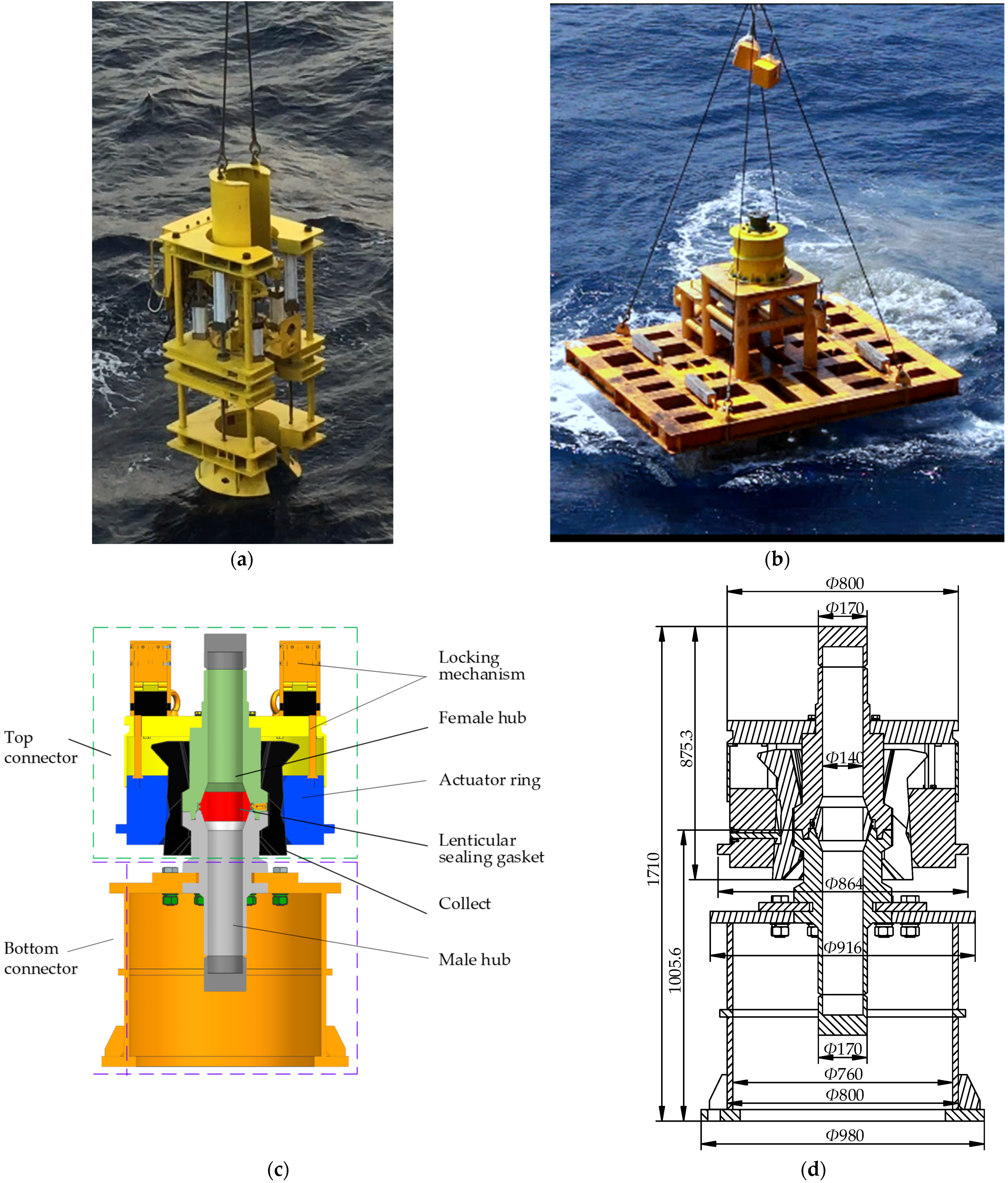
2. The Subsea Connector Structure
3. Thermal–Structural Coupling Mathematical Model of the Subsea Connector
3.1. Three-Dimensional Stress Caused by Steady Temperature Field
3.2. Three-Dimensional Stress Caused by Transient Temperature Field
3.3. Three-Dimensional Stress Caused by Internal Pressure
3.4. Thermal–Structural Coupling Stress
4. Numerical Simulation of Thermal–Structural Coupling of the Subsea Connector
4.1. Transient Temperature Field Analysis of the Subsea Connector
- The condition of uniform temperature rise: after 100 s, the internal surface temperature of the connector rises from 3 °C to 150 °C.
- The condition of uniform temperature drop: based on the steady temperature distribution, after 100 s, the internal surface temperature of the connector drops from 150 °C to 3 °C.
- The condition of instantaneous temperature drop: based on the steady temperature distribution, the internal surface temperature of the connector instantaneously drops to 3 °C.
- The condition of temperature shock: after 100 s, the internal surface temperature of the connector rises from 3 °C to 150 °C, and then after another 100 s, it drops from 150 °C to 3 °C.
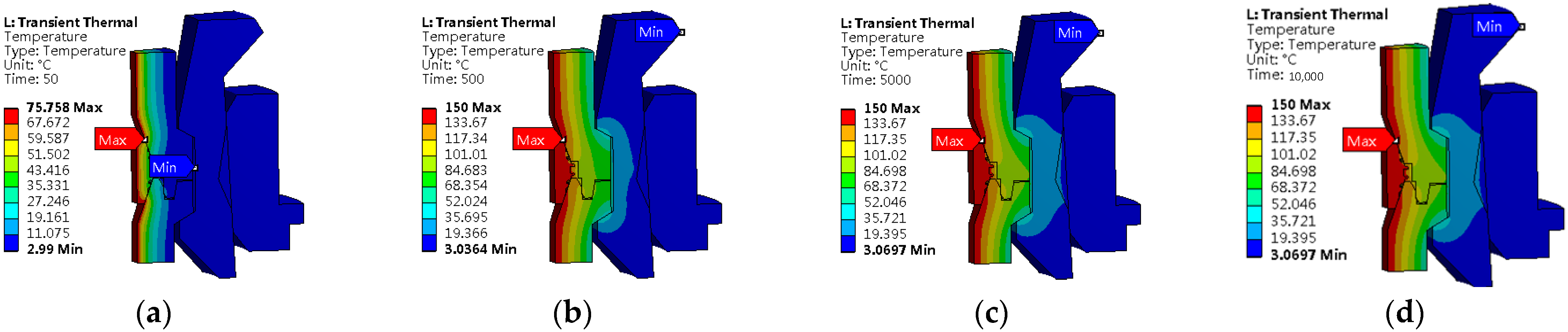
4.1.1. Analysis of Temperature Field under the Working Condition of Uniform Temperature Rise
- After 50 s, the oil–gas temperature inside the connector rises to 76.5 °C. The temperature of the inner wall of the hub and the inner wall of the LSG reaches 75.76 °C, and the heat is mainly concentrated on the LSG. The temperature of the hub close to its inner wall is relatively higher, and the temperature of the hub outer wall, clamp and actuator ring is the same as the temperature of seawater.
- After the temperature rising for 500 s, the oil–gas temperature reaches 150 °C and maintains for a period of time. The overall temperature of the LSG and hub increases significantly, and the heat is transferred to the collet through the outer wall of the hub.
- After the temperature rising for 5000 s, the heat is transferred to the actuator ring. However, the heat on the collet and actuator ring was mainly concentrated near the hub.
- Comparing the temperature field distributions at 5000 s and 10,000 s, the temperature field tends to be stable after the temperature rising for 5000 s.
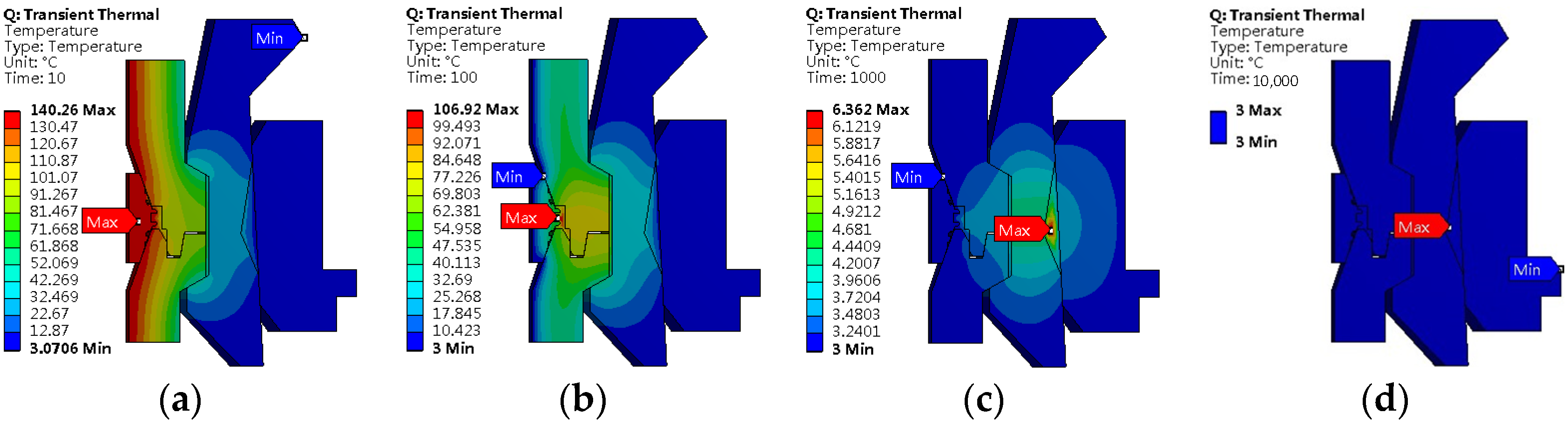
4.1.2. Analysis of Temperature Field under the Working Condition of Uniform Temperature Drop
- After the temperature dropping for 10 s, the transient maximum temperature (140.26 °C) is mainly on the LSG.
- After the temperature dropping for 100 s, the transient maximum temperature (106.92 °C) is concentrated in the seawater layer between the LSG and hub.
- After the temperature dropping for 1000 s, the transient heat was mainly concentrated in the seawater layer between the actuator ring and the collet, and the temperature is 6.362 °C.
- After the temperature dropping for 10,000 s, the overall temperature inside the connector has been reduced to seawater temperature.
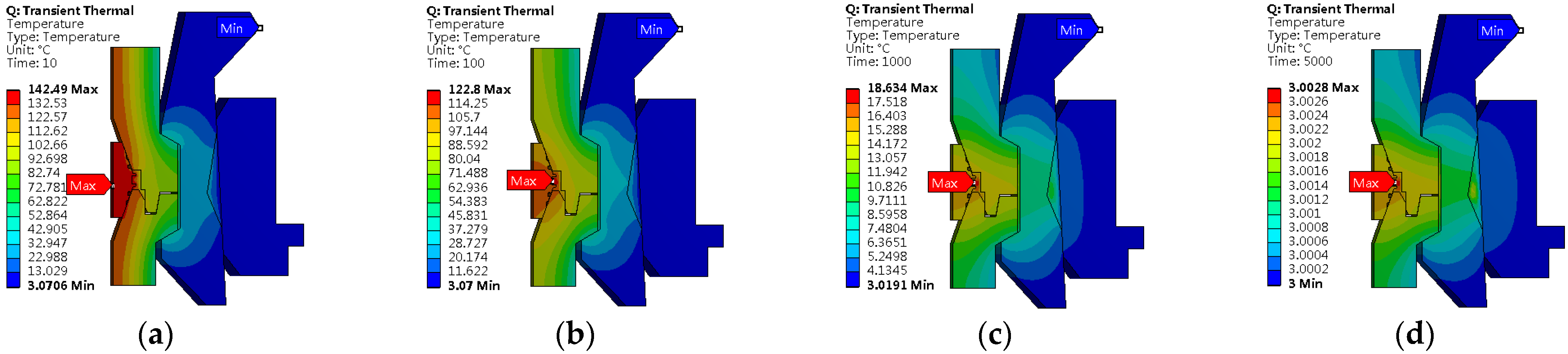
4.1.3. Analysis of Temperature Field under the Working Condition of Instantaneous Temperature Drop
- After the temperature dropping for 10 s, the maximum instantaneous temperature of the connector is concentrated at the LSG, which is 142.49 °C.
- After the temperature dropping for 100 s, compared with the temperature field figure at 10 s, it is found that after the oil–gas temperature is instantly removed, the inner wall of the hub and the inner wall of the LSG dissipate heat rapidity, and the temperature drops drastically. The heat is mainly concentrated at the junction of the outer wall of the LSG and seawater, and the maximum temperature is 122.8 °C; the temperature field distribution of the collet and actuator ring is similar to that at 10 s; however, the temperature is slightly lower.
- After the temperature dropping for 1000 s, the overall temperature inside the connector is relatively lower, and the highest temperature appears in the seawater layer between the LSG and hub, which is 18.634 °C.
- After the temperature dropping for 5000 s, the connector temperature is close to the seawater temperature, with a maximum temperature of merely 3.0028 °C.
4.1.4. Analysis of Temperature Field under the Working Condition of Temperature Shock
- After 10 s, the heat is mainly concentrated in the inner walls of the LSG and the hub, and the maximum temperature is 16.364 °C.
- After 30 s, the heat gradually diffuses to the outer walls of the LSG and the hub, with a maximum temperature of 46.061 °C.
- After 60 s, the temperature field distribution is similar to that at 10 s. However, the temperature is relatively higher, and the maximum temperature is 90.606 °C.
- After 200 s, the temperature is reduced to 3 °C. The heat is mainly concentrated at the hub, and the maximum temperature is reduced to 63.181 °C.
4.2. Analysis of Coupling Stress Calculation Examples under the Transient Temperature Field
4.2.1. Coupling Stress Analysis under the Working Condition of Temperature–Pressure Rise
4.2.2. Coupling Stress Analysis under the Working Condition of Temperature–Pressure Drop
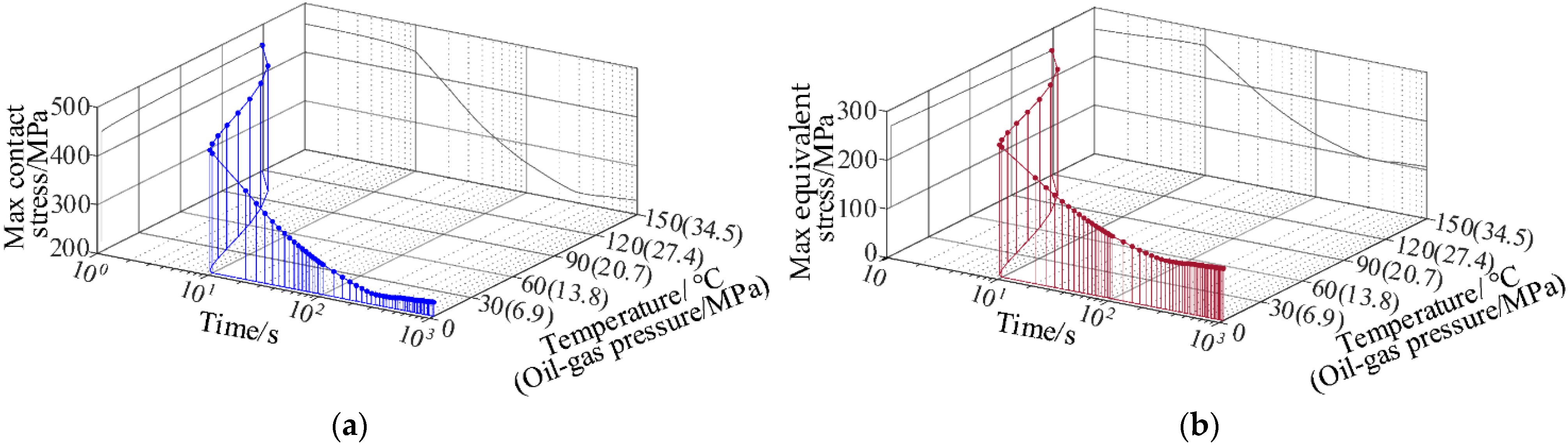
4.2.3. Coupling Stress Analysis under the Working Condition of Temperature–Pressure Instantaneous Drop
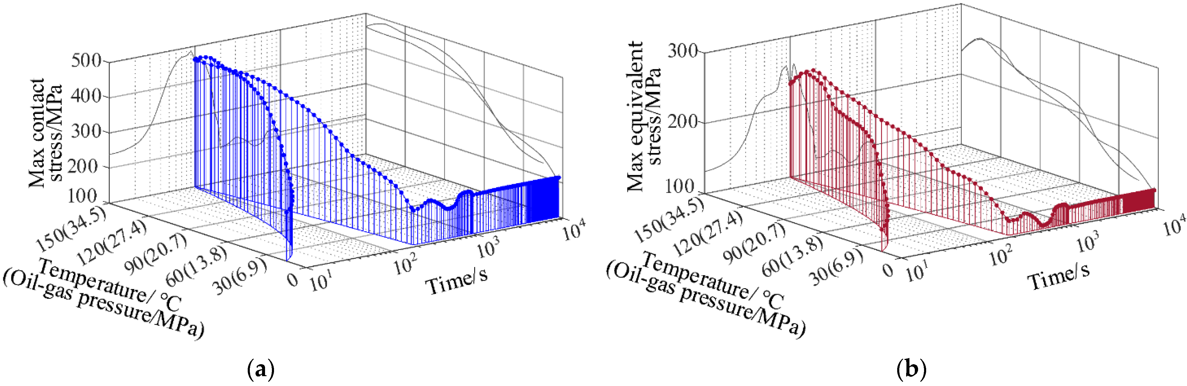
4.2.4. Coupling Stress Analysis under the Working Condition of Temperature-Pressure Shock
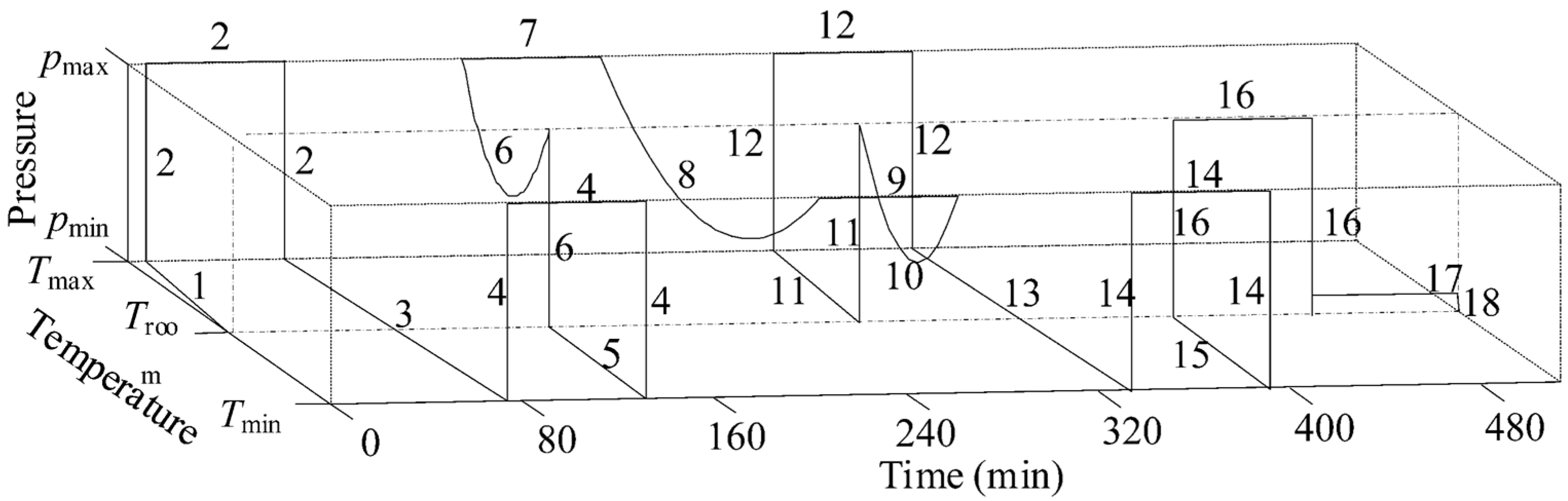
5. Temperature Cycle Test of Sealing Performance
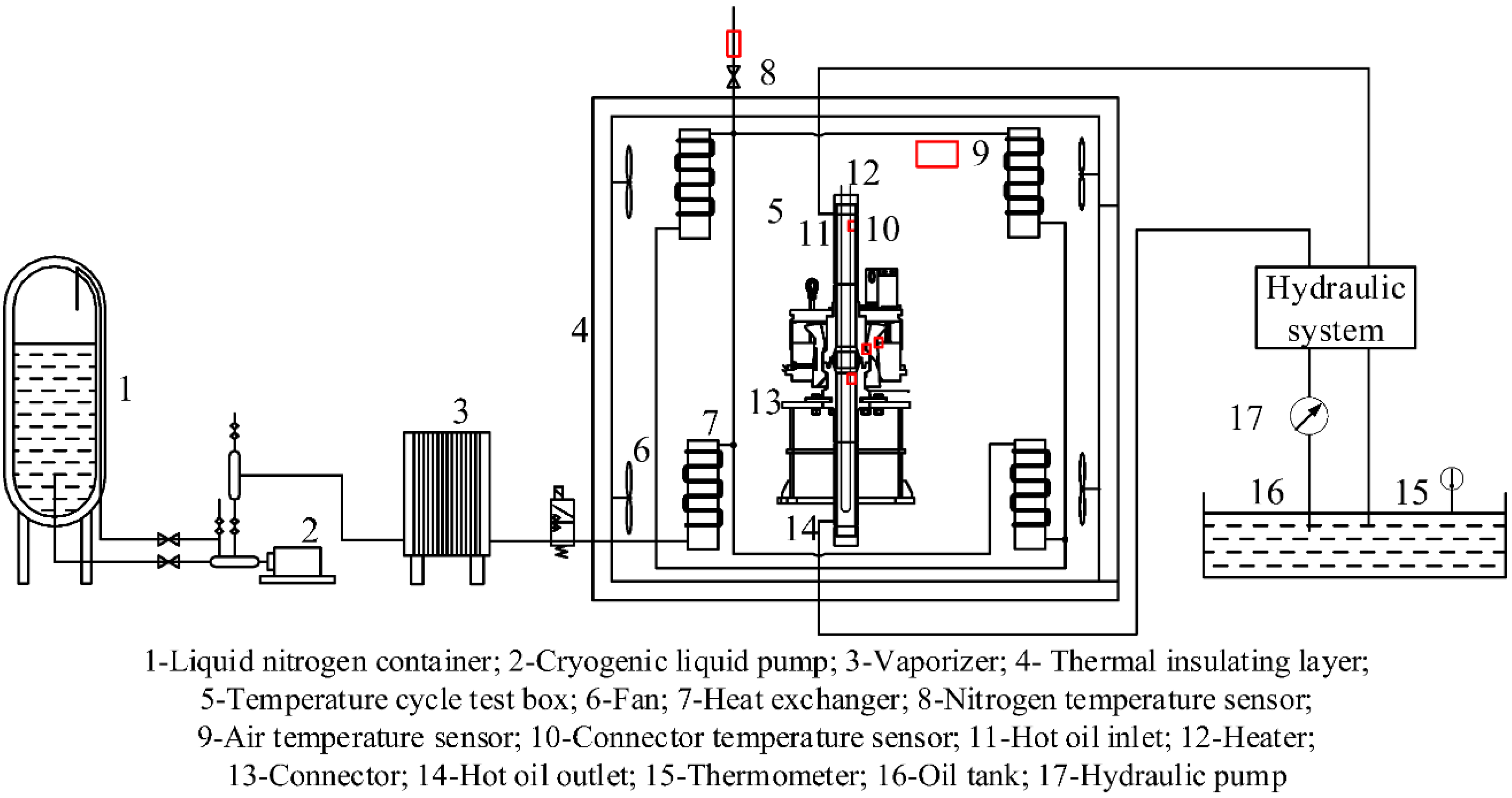
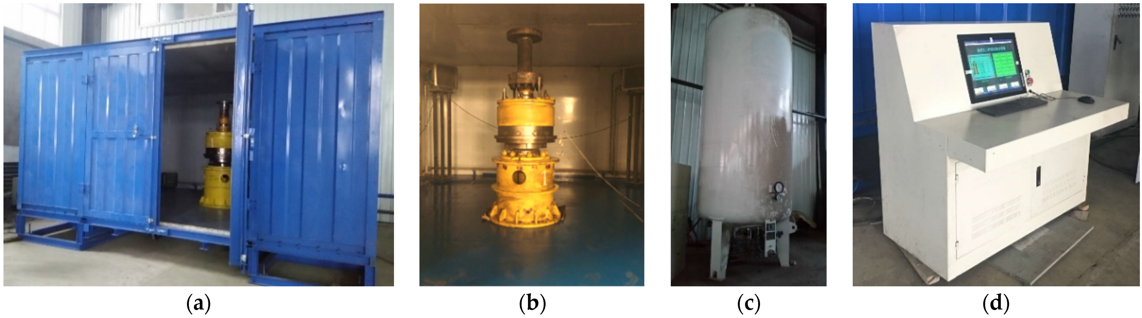
5.1. Temperature Cycle Test Device and Process
- The temperature of the temperature cycle test box outside the connector is set to 3 °C throughout, the initial temperature of the inner cavity of the connector is room temperature, and the internal pressure is 0 MPa. The inner cavity of the subsea collet connector is heated to 150 °C.
- Pressurize the connector cavity, increase the internal pressure to 34.5 MPa, hold the pressure for 60 min, and then depressurize to 0 MPa.
- Reduce the temperature of the connector cavity to 3 °C.
- Increase the internal pressure of the connector to 34.5 MPa, hold the pressure for 60 min, and then depressurize to 0 MPa.
- Increase the temperature of the connector cavity to room temperature.
- Increase the internal pressure of the connector to 34.5 MPa at room temperature and then raise the temperature of the connector cavity to 150 °C, maintaining the inner cavity pressure of the connector at more than 0.5 times of 34.5 MPa.
- Set the internal pressure of the connector to 34.5 MPa and hold it for 60 min.
- Reduce the temperature of the connector cavity to 3 °C and maintain the internal pressure of the connector at 34.5 MPa for more than 0.5 times during the temperature drop process.
- Set the internal pressure of the connector to 34.5 MPa and hold it for 60 min.
- Increase the temperature of the connector cavity to room temperature, maintain the internal pressure of the connector at more than 0.5 times 34.5 MPa during the temperature rise.
- Depressurize the connector to 0 MPa and raise the internal temperature of the connector from room temperature to 150 °C.
- Set the internal pressure of the connector to 34.5 MPa, hold it for 60 min, and then depressurize it to 0 MPa.
- Reduce the temperature of the connector cavity to 3 °C.
- Set the internal pressure of the connector to 34.5 MPa, hold it for 60 min, and then depressurize it to 0 MPa.
- Increase the temperature of the connector cavity to room temperature.
- Set the internal pressure of the connector to 34.5 MPa, hold it for 60 min, and then depressurize it to 0 MPa.
- Set the initial pressure in the connector cavity to 10% of 34.5 MPa, and then hold this pressure for 60 min.
- Depressurize the internal pressure of the connector to 0 MPa, and then end the test.
5.2. Analysis of Temperature Data
- It can be seen that the connector is pressure-held at different temperatures. The maximum pressure drop is 0.9 MPa in the second stage, which is 2.6% of the initial loading pressure and is within the allowable pressure settling range. After the temperature and pressure cycle loading test, the connector maintains a pressure of 3.5 MPa in the 17th stage. The pressure drop is 0.1 MPa, 2.86% of the initial loading pressure and less than 5% of the loading pressure. This shows that the connector still enjoys good sealing performance after temperature and pressure cycles.
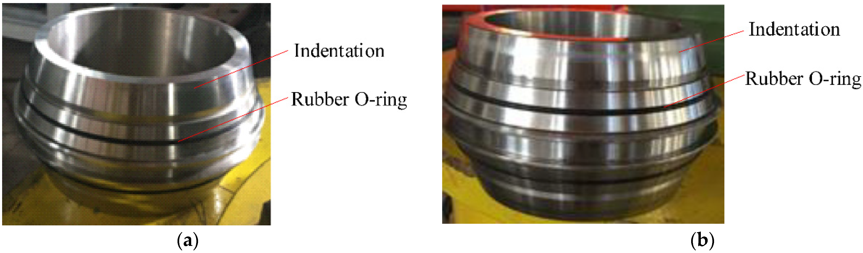
- A comparison of the composite LSG after the test is shown in Figure 13.
- Figure 13a shows the LSG after the hydrostatic pressure test of 1.5 times the rated internal pressure. The LSG has uniform indentation without disorderly wear and scratch. The seal width is approximately 2.17 mm measured by a vernier caliper with an accuracy of 0.1 mm; meanwhile, the rubber O-ring is in good shape without scratch and distortion.
- Figure 13b shows the LSG after the temperature cycle test. The LSG has pronounced indentation. There are some short scratches near the indentation, and the overall seal width seems to be increased. The width of the indentation and scratch is about 4.92 mm, which is 2.27 times that of the hydrostatic pressure test; through observation, the rubber O-ring is in good shape without excessive wear.
- The most obvious results emerge from the test is that under the multiple effects of temperature load, pressure load and preload, rapid temperature rising and dropping will lead to increasing wear of the spherical surface of the LSG. The composite sealing structure can effectively address the insufficient temperature compensation capacity of metal to ensure the sealing performance of the subsea collet connector under loads of temperature and pressure cycles.
6. Conclusions
- The transient thermal–structural coupling of the subsea connector was mathematically modelled. The mathematical modelling of transient thermal–structural coupling of the subsea connector was carried out. The calculation models of radial stress, circumferential stress and axial stress of the LSG under combined loads of the axial preload, internal oil–gas pressure and temperature were obtained.
- Numerical simulations of the transient temperature field of the subsea collet connector under four working conditions of uniform temperature rise, uniform temperature drop, instantaneous temperature drop, and temperature shock were carried out, and the study showed that: under each working condition, in the process of temperature variation from transient to steady distribution, the larger the temperature difference between the components, the greater the difference in expansion rate, the greater the impact on the sealing performance of the LSG.
- Numerical simulations of the working conditions of temperature–pressure rise, temperature–pressure drop, instantaneous temperature–pressure drop, temperature–pressure shock under the transient temperature field were carried out. The results showed that the smooth variation of oil–gas pressure and temperature had little impact on the sealing performance of the connector; when the temperature and oil and gas pressure varied suddenly, the maximum contact stress and equivalent stress of the sealing surface would fluctuate greatly, which was prone to fatigue and wear, and thus to affect the reliability of the sealing performance, this situation should be avoided.
- After the temperature cycle test, the final connector holding pressure drop is 2.86% of the initial loading pressure, indicating that the connector still enjoys good sealing performance after the temperature cycle. After the temperature cycle test, there is an increased seal width of the LSG. The rubber O-ring is in good shape without excessive wear.
Author Contributions
Funding
Institutional Review Board Statement
Informed Consent Statement
Conflicts of Interest
Appendix A
References
- Leffler, W.L.; Pattarozzi, R.; Sterling, G. Deepwater Petroleum Exploration & Production: A Nontechnical Guide, 2nd ed.; Pennwell Corp: Tulsa, OK, USA, 2011. [Google Scholar]
- Wang, W.; Yun, F.; Sun, H.; Wang, L.; Yan, Z.; Wang, G.; Gong, H.; Jiao, K.; Liu, D.; Hao, X. The Research and Experiments on Contact Sealing Theory of the Underwater Clamp Connector. Machines 2021, 9, 262. [Google Scholar] [CrossRef]
- Abid, M.; Ullah, B. Three-dimensional nonlinear finite-element analysis of gasketed flange joint under combined internal pressure and variable temperatures. J. Eng. Mech. 2007, 133, 222–229. [Google Scholar] [CrossRef]
- Abid, M.; Awan, A.W.; Nash, D.H. Determination of load capacity of a non-gasketed flange joint under combined internal pressure, axial and bending loading for safe strength and sealing. J Braz. Soc. Mech. Sci 2014, 36, 477–490. [Google Scholar] [CrossRef] [Green Version]
- Abid, M.; Khan, N.B. Behavior of gasketed bolted pipe flange joint under combined internal pressure, axial, and bending load: Three-dimensional numerical study. Proc. Inst. Mech. Eng. Part E J. Process Mech. Eng. 2018, 232, 314–322. [Google Scholar] [CrossRef]
- Abid, M.; Nash, D.H.; Javed, S.; Wajid, H.A. Performance of a gasketed joint under bolt up and combined pressure, axial and thermal loading—FEA study. Int. J. Press. Vessel. Pip. 2018, 168, 166–173. [Google Scholar] [CrossRef] [Green Version]
- Zhou, X.J.; Qiu, X.Q.; Zhang, B.; Chen, G.M. Finite Element Analysis of Bolted Flange Joint under Transient Temperature Field. Press. Vessel Technol. 2007, 24, 8–11, 16. [Google Scholar]
- Avanzini, A.; Donzella, G. A computational procedure for life assessment of UHP reciprocating seals with reference to fatigue and leakage. Int. J. Mater. Prod. Technol. 2007, 30, 33–51. [Google Scholar] [CrossRef]
- Omiya, Y.; Sawa, T. Thermal Stress Analysis and the Sealing Performance Evaluation of Bolted Flange Connection at Elevated Temperature. In Proceedings of the ASME 2009 Pressure Vessels and Piping Conference, Prague, Czech Republic, 26–30 July 2009. [Google Scholar]
- Omiya, Y.; Sawa, T. Stress Analysis and Sealing Performance Evaluation of Bolted Pipe Flange Connections With Smaller and Larger Nominal Diameter Under Repeated Temperature Changes. In Proceedings of the ASME 2014 Pressure Vessels and Piping Conference, Anaheim, CA, USA, 20–24 July 2014. [Google Scholar]
- Sawa, T.; Takagi, Y.; Torii, H. Effect of Material Properties of Gasket on the Sealing Performance of Pipe Flange Connections at Elevated Temperature. In Proceedings of the AMSE Pressure Vessels and Piping Conference, Boston, MA, USA, 19–23 July 2015. [Google Scholar]
- Luo, Y.Y.; Liu, X.Y.; Hao, J.; Wang, Z.; Lin, X.M. Research on thermal fatigue failure mechanism of aviation electrical connectors. Acta Armamentarii 2016, 7, 1266–1274. [Google Scholar] [CrossRef]
- Abdullah, O.I.; Schlattmann, J.; Jobair, H.; Beliardouh, N.E.; Kaleli, H. Thermal stress analysis of dry friction clutches. Ind. Lubr. Tribol. 2018, 72, 189–194. [Google Scholar] [CrossRef]
- Xue, J.L.; Chen, X.D.; Fan, Z.C.; Wang, L. Calculation of Leakage Rate for Bolted Flanged Joint during the Long Term Serice at High Temperature. In Proceedings of the AMSE Pressure Vessels and Piping Conference, Prague, Czech Republic, 15–20 July 2018. [Google Scholar]
- Zhang, L.; Xiao, G. Analysis of the metal-to-metal contact flange joint subject to external bending moment. Proc. Inst. Mech. Eng. Part E J. Process Mech. Eng. 2018, 233, 234–241. [Google Scholar] [CrossRef]
- Barsoum, I.; Barsoum, Z.; Islam, M.D. Thermomechanical Evaluation of the Performance and Integrity of a HDPE Stub-End Bolted Flange Connection. J. Press. Vessel. Technol. 2019, 141, PVT-18-1259. [Google Scholar] [CrossRef]
- Tang, L.P.; He, W.; Zhu, X.H.; Zhou, Y.L. Sealing Performance Analysis of an End Fitting for Marine Unbonded Flexible Pipes Based on Hydraulic-Thermal Finite Element Modeling. Energies 2019, 12, 2198. [Google Scholar] [CrossRef] [Green Version]
- Chen, J.; Ding, X.; Zhang, W.; Yan, R.; Sun, B. Fractal prediction model for the thermo-elastic normal contact stiffness of frictional interfaces in dry gas seals. J. Vib. Shock 2020, 39, 257–263, 284. [Google Scholar] [CrossRef]
- Li, Y.; Zhao, H.; Wang, D.; Li, X.; Zhao, T. Studied on Thermal Coupling and Sealing Characteristics of the Subsea Wellhead Connector Metal Seal. IOP Conf. Ser. Earth Environ. Sci. 2020, 527, 012005. [Google Scholar] [CrossRef]
- Wang, Q.; Hu, Y.P.; Ji, H.H. Leakage, heat transfer and thermal deformation analysis method for contacting finger seals based on coupled porous media and real structure models. Proc. Inst. Mech. Eng. Part C J. Mech. Eng. Sci. 2020, 234, 2077–2093. [Google Scholar] [CrossRef]
- Zhang, H.; You, H.; Lu, H. Mechanical–thermal sequential coupling simulation for predicting the temperature distribution of seal rings—Part I. Seal. Technol. 2020, 2020, 5–8. [Google Scholar] [CrossRef]
- Zhang, H.; You, H.; Lu, H. Mechanical–thermal sequential coupling simulation for predicting the temperature distribution of seal rings—Part II. Seal. Technol. 2020, 2020, 5–9. [Google Scholar] [CrossRef]
- Zeng, W.; Xue, Y.X.; Sun, Y.H.; Zhao, J.; Xie, H.; Ren, T. Sealing reliability assessment of deep-water oil and nature gas pipeline connector considering thermo-mechanical coupling. Proc. Inst. Mech. Eng. Part M J. Eng. Marit. Environ. 2021, 1, 196–208. [Google Scholar] [CrossRef]
- Liu, H.; Rao, Z.; Pang, R.; Zhang, Y. Research on Thermal Characteristics of Ball Screw Feed System Considering Nut Movement. Machines 2021, 9, 249. [Google Scholar] [CrossRef]
- Zhang, Y.; Wang, G.; Pan, X.; Li, Y. Calculating the Load Distribution and Contact Stress of the Disposable Harmonic Drive under Full Load. Machines 2022, 10, 96. [Google Scholar] [CrossRef]
- Song, J.H.; Kang, S.W.; Kim, Y.J. Optimal design of the disc vents for high-speed railway vehicles using thermal-structural coupled analysis with genetic algorithm. Proc. Inst. Mech. Eng. Part C J. Mech. Eng. Sci. 2021, 11, 09544062211059112. [Google Scholar] [CrossRef]
- Wen, M. An Analysis of the Coupling Between Temperature and Thermal Stress of Disc Brakes Based on Finite Element. Int. J. Heat Technol. 2021, 39, 1819–1827. [Google Scholar] [CrossRef]
- Gao, L.; Zhao, X.C.; Wang, B. Thermostructural Responses of Metallic Lattice-Frame Sandwich Structure for Hypersonic Leading Edges. J. Thermophys. Heat Transf. 2021, 35, 708–714. [Google Scholar] [CrossRef]
- Ma, H.Q.; Jia, J.W.; Ding, R.X.; Luo, X.M.; Peng, D.G.; Hou, C.Q.; Wang, G.; Zhang, Y.J. Numerical investigation on fatigue life of aluminum brazing structure with fin-plate-side bar under the low temperature thermal-structure cyclic stress. Eng. Fail. Anal. 2022, 131, 18. [Google Scholar] [CrossRef]
- Hetnarski, R.B. Encyclopedia of Thermal Stresses; Springer: Dordrecht, The Netherlands, 2014. [Google Scholar]
- Cheng, X.; Peng, W.; Sun, L.; Li, X.; Yin, Z. Analysis of the fracture pattern and failure time of LNG outer tanks under the action of thermal load. Nat. Gas Ind. 2015, 35, 103–109. [Google Scholar] [CrossRef]
- Lu, G.C.; Chu, G.N. Research of Directional Stress Distribution on the Fully Plastic Bulged Pressure Hull. Adv. Mater. Res. 2015, 1082, 412–415. [Google Scholar] [CrossRef]


| Temperature (°C) | Heat Capacity (J∙kg−1∙K−1) | Elastic Modulus (MPa) | Thermal Expansion Coefficient (°C−1) | Thermal Conductivity (W∙m−1∙K−1) | Poisson’s Ratio |
|---|---|---|---|---|---|
| 20 | 3.603 | 2.06 × 10⁵ | 1.64 × 10⁻⁵ | 14.7 | 0.25 |
| 50 | 3.744 | 1.970 × 10⁵ | 1.65 × 10⁻⁵ | 15.2 | 0.25 |
| 100 | 3.901 | 1.955 × 10⁵ | 1.68 × 10⁻⁵ | 15.8 | 0.25 |
| 150 | 4.103 | 1.915 × 10⁵ | 1.70 × 10⁻⁵ | 16.7 | 0.25 |
| Temperature (°C) | Heat Capacity (J∙kg−1∙K−1) | Elastic Modulus (MPa) | Thermal Expansion Coefficient (°C−1) | Thermal Conductivity (W∙m−1∙K−1) | Poisson’s Ratio |
|---|---|---|---|---|---|
| 20 | 3.603 | 2.1 × 10⁵ | 1.64 × 10⁻⁵ | 14.7 | 0.3 |
| 50 | 3.744 | 1.970 × 10⁵ | 1.65 × 10⁻⁵ | 15.2 | 0.3 |
| 100 | 3.901 | 1.955 × 10⁵ | 1.68 × 10⁻⁵ | 15.8 | 0.3 |
| 150 | 4.103 | 1.915 × 10⁵ | 1.70 × 10⁻⁵ | 16.7 | 0.3 |
| Percentage of Temperature Drop (%) | Time for Temperature Drop (s) | ||||
|---|---|---|---|---|---|
| LSG | Female Hub | Male Hub | Collet | Actuator Ring | |
| 20 | 14.4 | 124 | 74.4 | 102 | 274 |
| 40 | 19.4 | 174 | 114 | 154 | 464 |
| 60 | 23.4 | 234 | 164 | 264 | 974 |
| 80 | 27.4 | 354 | 264 | 364 | 1230 |
| 90 | 194 | 505 | 400 | 584 | 1770 |
| 100 | 3170 | 3870 | 3670 | 3570 | 3470 |
| Percentage of Temperature Drop (%) | Time for Temperature Drop (s) | ||||
|---|---|---|---|---|---|
| LSG | Female Hub | Male Hub | Collet | Actuator Ring | |
| 20 | 102 | 200 | 144 | 164 | 324 |
| 40 | 224 | 344 | 284 | 324 | 505 |
| 60 | 405 | 534 | 474 | 534 | 724 |
| 80 | 724 | 874 | 800 | 934 | 1050 |
| 90 | 1050 | 1240 | 1140 | 1640 | 1440 |
| 100 | 6870 | 6770 | 6770 | 6370 | 5770 |
| Name of Component | Peak Temperature (°C) | Generation Time (s) | Lag Time (s) |
|---|---|---|---|
| LSG | 105.37 | 118.02 | 18.02 |
| Female hub | 36.112 | 190.83 | 90.83 |
| Male hub | 54.438 | 140.83 | 40.83 |
| Collet | 18.352 | 170.83 | 70.83 |
| Actuator ring | 4.0547 | 305 | 205 |
| Case | Load Condition | ||
|---|---|---|---|
| Axial Preload | Transient Temperature Load | Oil-Gas Pressure Load | |
| Temperature-pressure rise | 63.8 kN |  |  |
| Temperature-pressure drop | 63.8 kN | 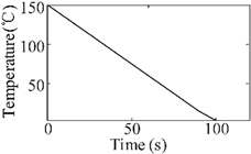 | 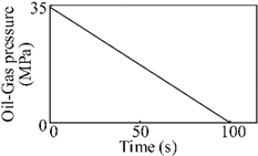 |
| Temperature-pressure instantaneous drop | 63.8 kN |  |  |
| Temperature-pressure shock | 63.8 kN | 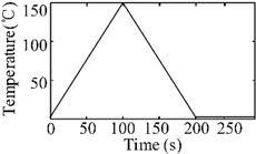 | 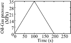 |
| Steps | Temperature (°C) | Pressure (MPa) | Holding Pressure (min) | Pressure Drop (MPa) |
|---|---|---|---|---|
| 1 | 20.8–150.2 | 0 | - | - |
| 2 | 150.2 | 34.6 | 60 | 0.9 |
| 3 | 150.2–3.1 | 0 | - | - |
| 4 | 3.1 | 34.8 | 60 | 0.2 |
| 5 | 3.1–20.2 | 0 | - | - |
| 6 | 20.2–151.0 | 17.3–34.0 | - | - |
| 7 | 151.0 | 34.5 | 60 | 0.7 |
| 8 | 151.0–3.3 | 17.9–34.2 | - | - |
| 9 | 3.3 | 34.5 | 60 | 0.5 |
| 10 | 3.3–20.5 | 17.5–34.6 | - | - |
| 11 | 20.5–152.8 | 0 | - | - |
| 12 | 152.8 | 34.8 | 60 | 0.7 |
| 13 | 152.8–3.1 | 0 | - | - |
| 14 | 3.1 | 34.2 | 60 | 0.6 |
| 15 | 3.1–21.9 | 0 | - | - |
| 16 | 21.9 | 34.6 | 60 | 0.1 |
| 17 | 21.9 | 3.5 | 60 | 0.1 |
| 18 | 21.9 | 0 | - | - |
Publisher’s Note: MDPI stays neutral with regard to jurisdictional claims in published maps and institutional affiliations. |
© 2022 by the authors. Licensee MDPI, Basel, Switzerland. This article is an open access article distributed under the terms and conditions of the Creative Commons Attribution (CC BY) license (https://creativecommons.org/licenses/by/4.0/).
Share and Cite
Liu, D.; Yun, F.; Wang, W.; Jiao, K.; Wang, L.; Yan, Z.; Jia, P.; Wang, X.; Liu, W.; Sun, H.; et al. Sealing Contact Transient Thermal-Structural Coupling Analysis of the Subsea Connector. Machines 2022, 10, 213. https://doi.org/10.3390/machines10030213
Liu D, Yun F, Wang W, Jiao K, Wang L, Yan Z, Jia P, Wang X, Liu W, Sun H, et al. Sealing Contact Transient Thermal-Structural Coupling Analysis of the Subsea Connector. Machines. 2022; 10(3):213. https://doi.org/10.3390/machines10030213
Chicago/Turabian StyleLiu, Dong, Feihong Yun, Wuchao Wang, Kefeng Jiao, Liquan Wang, Zheping Yan, Peng Jia, Xiangyu Wang, Weifeng Liu, Haiting Sun, and et al. 2022. "Sealing Contact Transient Thermal-Structural Coupling Analysis of the Subsea Connector" Machines 10, no. 3: 213. https://doi.org/10.3390/machines10030213