Investigation of the Effect of Rope Cutter on Water Flow behind Ship Propellers Based on CFD Analysis

Abstract

Small vessels operating in coastal waters are susceptible to propeller failure because of the entanglement of marine debris. Secondary accidents such as the injury of divers may also occur when removing entangling material. Rope cutters are devices used to prevent marine litter from entangling the propeller of small ships. However, installing rope cutters on propeller shafts might affect the working of the propeller. In this study, three-dimensional simulations were performed to investigate the effect of a rope cutter on flow characteristics behind the propeller. The Computational fluid dynamics (CFD) models were validated by particle image velocimetry (PIV) experiments performed in a rope cutter performance testing tank. The study results showed that the installation of a rope cutter on the propeller shaft led to an insignificant reduction in water flow velocity magnitude behind the propeller. Additionally, the effects of the rope cutter on the reductions of thrust (0.87%) and torque (0.76%) of the propeller were also negligible. However, it is very interesting to note that rope cutter installation resulted in a lower vortex formation, leading to a significant reduction in the turbulence intensity behind the propeller by 27.12%, 37.50%, and 47.29% at 100, 150, and 200 rpm propeller speed, respectively. Based on the study results, it can be concluded that rope cutters help to reduce propeller entanglements without significantly affecting the propeller’s working.

1. Introduction

Marine debris, such as fishing gear, ropes, and other non-biodegradable remains at sea, is of great concern as it can lead to navigational hazards and imposes economic loss to the related industries [1,2,3]. Marine debris in the ocean is caused by loss; intentional abandonment of the nets by fishermen; or discarded fishing nets because of excessive fishing gear, illegal fishing, gear conflicts, and costs of onshore disposal [3]. Such debris poses substantial challenges to small ships navigating within coastal areas. The primary challenges include propeller entanglement, resulting in a reduction in stability and navigability of ships, which could lead to marine collisions; schedule delays; or secondary accidents such as diver injury that can occur during the removal of entangled material from the propeller [3]. In short, propeller failure due to debris entanglement could result in significant financial losses and/or crew injury [2,3,4,5].

There are numerous reports regarding ship collisions, engine damage, or even human deaths caused by debris entanglement at sea [5,6,7,8]. The number of accidents is forecast to increase even more significantly due to the increasing number of small boats operating in coastal waters, increasing human activities at sea, and competitive fishing activities resulting in more fishing nets being left in the sea.

In order to prevent propeller entanglement, rope cutters were invented. They are safety devices designed and installed on propeller shafts to cut foreign objects from coiling on ships’ propellers [9]. The device consists of rotating blades and fixed blades. The rotating blades are installed on the propeller shaft while the fixed blades are installed on the stern tube of the shaft to cut off any marine debris that may flow towards the propeller by scissors principle.

Some research has been performed to investigate the usefulness, safety, and performance of rope cutter devices. Lee et al. reported in [8] that the average number of accidents per year after rope cutter installations was only 1.34 times compared to 6.15 times before installing rope cutters. This means that rope cutter installation helped to reduce more than 78% of accident possibilities related to marine debris. Lee et al. [10] also performed a study on the effect of rope cutters on the vibration of the propeller shaft. The results of the study showed that the effect of the cutting action on the propeller shaft vibration was found to be very small. Therefore, installing a rope cutter on the propeller shaft has almost no effect on the operation of the propeller. In addition, Kim et al. [11] performed a research study on the structural stability and the effectiveness of a scissor-type rope cutter using the finite element analysis. They found that the propeller shaft was not rotated by the rope entanglement. The results also revealed that the developed rope cutter structure enables hassle-free removal of ropes and fishing nets in all operational conditions.

Through the literature reviews above, even though there were some studies related to rope cutters, it is very rare to find studies on the effect of rope cutters on the water flow behind the ship’s propeller when installed on propeller shafts. That is why this study needs to be carried out.

Flow field study is of special interest to many researchers, therefore, computational and experimental fluid dynamics technologies have advanced significantly. In previous decades, Laser Doppler Velocimetry (LDV) technique was widely used to investigate complex flows of propellers, mainly the turbulence characteristics [12,13]. Particle image velocimetry (PIV) is an analysis method used to map two-dimensional velocity distribution quantitatively and it provides us with vector information on particle pathways by tracking the displacement of seeding particles added in the flow field. To illuminate the seeding particles, Mie scattering, Rayleigh scattering, and shadowgraphy have generally been utilized. Mie scattering is a method of elastic scattering of light from seeding particles, and the scattering signal is much stronger than Rayleigh scattering since the direction of the scattering light is biased [14]. Therefore, the flow velocity measurement employing Mie scattering with a thin laser beam sheet is known to be a very effective diagnostic method in complex flows such as water flow behind propellers.

PIV analysis is a powerful experimental fluid dynamic technique that eliminates shortcomings experienced using the LDV technique. LDV shortcomings include: inability to provide the spatial characteristics of large coherent structures due to its single point measurement, error induction on the intensity of unsteady vertical structures due to its fixed location and time-averaging nature, and expensive testing cost because LDV requires long periods of operation to be able to obtain a whole velocity field [15]. On the other hand, PIV technique can record velocity information for a large number of spatial points in the same transient state, providing flow field structure and characteristics. Calcagno et al. [15] investigated a five-blade MAU propeller wake behind a ship model using stereo particle image velocimetry in a large free surface cavitation tunnel. The investigation pointed out the capability of stereo-PIV in resolving the complexity of the flow field. Paik et al. [16] used a two-frame particle image velocimetry to investigate wake properties behind a marine propeller with four blades at a high Reynolds number. An investigation of the wake behind a rotating propeller using PIV successfully analyzed wake characteristics, making PIV one of the most powerful tools for flow field experiments. As mentioned earlier, PIV has been used to analyze the flow field behind the propeller based on these excellent features, but PIV experiments performed under conditions before and after the rope cutter installation have not been reported yet.

Computational fluid dynamics (CFD) provide an effective and inexpensive means to numerically study the flow characteristics of fluids. CFD has shown powerful capabilities in the prediction and analysis of flow-related problems. Morgut and Nobile [17] performed a numerical prediction of the flow around marine propellers, working in a uniform inflow using different mesh types and turbulence models. The simulation results showed that, even though different meshes and different turbulence models led to a slight difference in the final CFD results, they still agreed well with the experimental data. Çelik [18] performed a numerical study to calculate the effect of the wake equalizing duct (WED) on the propulsion performance of a chemical tanker using a CFD tool based on the solution of Reynolds-averaged Navier–Stokes (RANS) equation. Analyzing the study results, they found out the slight effect of the WED on the ships’ resistance. They also revealed that additional 10% thrust was produced by WED. Seol [19] numerically analyzed the pressure fluctuations induced by the propeller sheet cavitation using their newly developed time domain method. The simulation results showed that the pressure fluctuation induced by propeller sheet cavitation was not simply proportional to the second derivative of the cavitation volume variation but inversely proportional to the distance. Through these literature reviews, it can be observed that CFD method has been successfully used to analyze the fluid flow around rotating propeller blades and would, therefore, be suitable for investigating the effect of rope cutters on the fluid flow behind the ship’s propeller in our current study.

In this study, water flow simulations around the propeller blades were performed using ANSYS Fluent code (ANSYS Inc., Canonsburg, PA, USA) to investigate the effect of a rope cutter installed on the ship’s propeller shaft on the water flow behind the propeller. The simulation results were validated using the PIV experiment results conducted in our laboratory.

2. CFD Numerical Analysis

This study investigates the effect of rope cutters installed on ships’ propeller shafts, on the water flow behind ships’ propellers operating in coastal waters using the CFD method. Since there were no experimental results available for CFD models validation purposes, we needed to conduct PIV experiments. Due to the feature of the PIV method, it is impossible to perform a PIV experiment in big areas of water (lake, river, or sea …). Therefore, we built a rope cutter testing tank for PIV experiments, which is explained in detail in later sections.

2.1. Study Procedure

The study procedure in this study included five steps:

-

Step 1: Pre-processing: creating the computational domain and mesh. Setting up the CFD models based on the physical features of the problems.

-

Step 2: Processing: calculating the solution.

-

Step 3: Post-processing: Analyzing and reporting the results. Validating the CFD models by comparing the simulation results to the experimental results.

-

Step 4: Solving the specified problems: after the CFD models are successfully validated, they are applied to simulate problems such as the one solved in the validation section.

-

Step 5: Analyzing and exporting the final results: the simulation results in all simulation cases are compared to state the final conclusions.

To validate the CFD models used in the study, CFD simulation along with a PIV experiment of propeller operation with a rope cutter (WRC) installed on the propeller shaft rotating at 100 rpm (revolution per minute) were performed. The validated CFD models were applied to the other simulations in the study.

2.2. Step 1—Pre-Processing

2.2.1. Computational Domain

In this study, the 3D model geometry for CFD simulations was built by the AutoCAD 2019 software (Autodesk, Inc., San Rafael, CA, USA). The computational domain was divided into two parts, a rotating part consisting of the propeller and rope cutter, and the remaining tank region was assigned as a stationary part. The computational domain has a length of 1200 mm, a width of 794 mm, and a height of 857 mm. Figure 1 shows the 3D model geometry for CFD simulations. Its dimensions correspond to those in the PIV experiment described in Section 2.5.2 below.

The propeller in this study is a standard HYDRAPOISE 3.45 propeller made of bronze. Where, number 3 represents the number of blades, while 0.45 is the blade area ratio. This is the ratio of the projected area of the blades to the area of a circle that the blades sweep (λ = 0.45). This type of propeller is ideal for small ships such as fishing ships. The main propeller dimensions, the installation position, and the structure of the rope cutter are shown in Figure 2 and Figure 3, respectively. Figure 3a shows rope cutter dimensions, where, blade to blade diameter (D_b) = 82 mm, rope cutter hub outer diameter (D_o) = 48 mm, rope cutter thickness (t) = 16 mm, rotating blade height B_h = 17 mm, and the inner diameter (D_i) = 30 mm. Propeller’s principal dimensions are shown in

Table 1. Principle propeller properties.

Propeller Properties	Dimensions [Unit: mm]
Propeller type Material Number of blades Propeller diameter (Dp [mm]) Propeller pitch (P [mm]) Hub diameter (Dh [mm]) Propeller hub length (Lh [mm]) Blade area ratio (λ [-]) Pitch/Diameter (P/Dp [-]) Hub diameter ratio (Dh/Dp [-])	Standard HYDRAPOISE 3.45 Right-handed Fixed Pitch Propeller (FPP) Bronze 3 360 254 65 88 0.45 0.7056 0.1806

.

2.2.2. Computational Mesh

The 3D computational mesh was generated using the ANSYS Meshing platform provided by ANSYS Workbench (ANSYS Inc., Canonsburg, PA, USA). A global meshing approach using an element size of 0.008 m was applied to generate computational meshes. The computational mesh cells were refined in the areas close to the propeller blades, shaft, and rope cutter in the rotation region to ensure an accurate prediction of fluid flow behavior near the walls. The cell size was then gradually increased in the direction away from the propeller, shaft, and rope cutter to reduce the number of elements to reduce calculation time. To improve the mesh quality and thus the result accuracy, sufficient mesh refinement was also established on the interfaces. A very fine mesh for the regions nearby the rope cutter and propeller blade walls was also created to get both high mesh quality and small element sizes nearby the walls to eliminate the near-wall effects on the fluid flow behavior.

In this study, fully tetrahedron, unstructured mesh was applied to the entire geometry. The unstructured tetrahedron mesh was specifically selected for this study because of its ability to discretize complex geometries with fast and minimum user intervention. A good mesh quality indicated by good mesh metrics was ensured before proceeding to the solution calculation. The whole computational mesh and the rotating domain of the mesh are shown in Figure 4a,b, respectively. A zoom-in area of the rotating mesh containing the propeller and rope cutters is shown in Figure 4c. The properties of the computational mesh are shown in

Table 2. Computational meshing properties.

Mesh Property	Details
Global element size Mesh type No. of Nodes No. of Elements Max. Aspect ratio Max. Skewness quality Min. Orthogonal quality	0.008 m Tetra type 143,316 758,316 19.371 0.79205 0.47

.

2.2.3. CFD Setup

CFD Models and Governing Equations

The accuracy of the CFD results obtained from a single-phase numerical simulation mainly depends on the turbulence model used. No turbulence model has been proved to be more powerful than others, but each model exhibits different levels of accuracy depending on the boundary conditions and the flow characteristics of the case under simulation. The k-ε model has been widely used by researchers in a wide range of flow simulations, including combustion, prediction of bubble column internal flow fields, propeller flow fields, etc. Since its proposal by Launder and Spalding [20], k-ε has formed a basis of flow simulation with its advantage of robustness, economy, and reasonable accuracy over a wide range of turbulent flows. Kutty and Rajendran [21] used the standard k-ε to predict the performance of a small advanced precision composite (APC) slow flyer propeller. The study showed that the standard k-ε produced good final prediction results. In addition, the k-ε turbulence model has also been widely used in cyclonic column simulations. Khan et al. [22], using a 3D geometry model for a bubble column, simulated using k-ε and RSM models. They also performed Laser Doppler anemometry measurements to validate their simulation. Consequently, they found out that k-ε and RSM models could be effectively used to predict the bubble column internal flow fields. Therefore, in this study, k-ε turbulence model was also used. This model is based on the transportation equations for turbulent kinetic energy, k, and its dissipation rate, ε [20].

The 3D fluid dynamic problem in our study is governed by the Navier–Stokes equations and continuity. Therefore, the Reynolds-averaging approach for turbulence was applied in this study. The Navier–Stokes equations for continuity and momentum are written in the Cartesian tensor as shown in Equations (1) and (2), respectively. Explanations of the variables are presented in the nomenclature section at the end of the article.

$$\frac{\partial u_i}{\partial x_i}=0$$

(1)

$$\frac{\partial \left(\rho u_i\right)}{\partial t}+\frac{\partial \left(\rho u_i{u}_j\right)}{\partial x_j}=-\frac{\partial P}{\partial x_i}+\frac{\partial }{\partial x_j}\left[\mu \left(\frac{\partial u_i}{\partial x_j}+\frac{\partial u_j}{\partial x_i}-\frac{2}{3}{\delta }_{ij}\frac{\partial u_l}{\partial x_l}\right)\right]+\frac{\partial }{\partial x_j}\left(\rho u_i^{\prime }{u}_j^{\prime }\right)$$

(2)

The model transport equation for k is derived from the exact equation, while the model transport equation for ε is obtained using physical reasoning. The k-ε derivation assumes that the flow is fully turbulent and the effect of the molecular viscosity is negligible. The turbulence kinetic energy, k, and its rate of dissipation equations for the k-ε model are given by ε, which are obtained from the transport Equations (3) and (4), respectively.

$$\frac{\partial \left(\rho k\right)}{\partial t}+\frac{\partial \left(\rho k{u}_i\right)}{\partial x_i}=\frac{\partial }{\partial x_i}\left[\left(\mu +\frac{{\mu }_t}{{\sigma }_k}\right)\frac{\partial k}{\partial x_j}\right]+G_k+G_b-\rho \epsilon -Y_M+S_k$$

(3)

$$\frac{\partial \left(\rho \epsilon \right)}{\partial t}+\frac{\partial \left(\rho \epsilon u_i\right)}{\partial x_i}=\frac{\partial }{\partial x_i}\left[\left(\mu +\frac{{\mu }_t}{{\sigma }_{\epsilon }}\right)\frac{\partial \epsilon }{\partial x_j}\right]+\frac{C_{1\epsilon }\epsilon }{k}\left(G_k+C_{3\epsilon }{G}_b\right)-\rho C_{2\epsilon }\frac{{\epsilon }^2}{k}$$

(4)

The CFD solution was performed using the pressure-based approach. The pressure-velocity coupling was achieved using a coupled algorithm. The second-order upwind scheme was used for pressure and momentum. The least-squares cell based was used for the gradient while the first-order upwind was used for both the turbulence kinetic energy and the turbulence dissipation rate. The coupled algorithm was more suitable due to the slightly larger time step used in this study. For convergence criteria, in this problem, absolute convergence criteria of 0.001 for continuity, velocity, k, and epsilon were set. These criteria are technically suitable for most problems, including single-phase, standard k-ε model problems as the same as in this study [23].

Boundary and Initial Conditions

The rotating action of the propeller and rope cutter was modeled by a sliding mesh. Unlike the moving reference frame (MRF) technique, the sliding mesh technique involves rotating the sub-domain containing the rotating components of the simulation (that is the propeller and rope cutter rotating blades in this study). In addition, sliding mesh produces an accurate time simulation where a strong fluid-propeller interaction is considered [24,25,26]. The sliding mesh approach is suitable for this study since it allows a good interaction between the rotating and stationary domains.

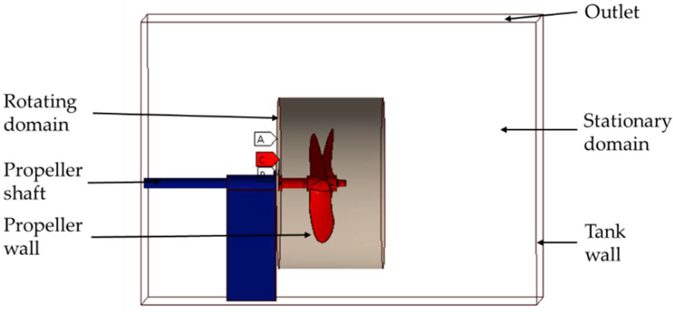
The rotating domain (with the sliding mesh) was specified by a smaller cylinder enclosing the entire propeller and the rotating blades of the rope cutter. The stationary domain represented the entire tank fluid domain. Various propeller rotational speeds (i.e., 100, 150, and 200 rpm) were assigned to the sliding mesh of the rotating domain in each case of the simulation. The interface between the rotational and the stationary domains will undergo a local transformation to enable the flow variables from one domain to another. The boundary and initial conditions, as well as the CFD model setup for simulation, was declared in the ANSYS Fluent solver for calculating the solution. The obtained results were finally analyzed using the CFD-post platform.

For the CFD models validation purpose, the boundary and initial conditions for simulations were assigned based on the actual working condition of the propeller and rope cutter in the PIV experiments. All the lower tank walls were set to wall boundary conditions. The top boundary of the computational domain was set as the pressure outlet boundary because the rope cutter performance tank top part is an open surface. The rest of the tank walls were set as walls. The rotating domain (assigned as a sliding mesh in the meshing process) was set to a constant rotational speed around the x-axis of 100, 150, and 200 rpm. The boundary conditions of the computational domain are shown in Figure 5.

2.3. Step 2—Processing

The simulations were conducted using ANSYS Fluent Solver. They were performed in parallel on an Intel(R) Core(TM) i9-10900X CPU @ 3.70GHz 3.70 GHz, 64 GB RAM windows workstation. In this study, each simulation was conducted for 16 propeller revolutions to ensure stable propeller conditions before analyzing the effect of the rope cutter on the flow behind the propeller. The time step size was maintained at 0.001 s throughout all simulation cases. The number of time steps for each simulation case was adjusted according to the propeller speed to ensure the same number of propeller revolutions (16 revolutions) in all simulation cases. Fifty maximum iterations per time step were set to ensure solution convergence. Monitoring the residuals showed that the solution reached convergence after around 35 iterations per each time step, and the computation was then skipped to the next time step. After finishing the calculation, the simulation results were post-processed for the CFD validation purpose.

2.4. Step 3—Post-Processing

2.4.1. Mesh Independence Analysis

Mesh quality, which is influenced by mesh resolution, plays an important role in the accuracy of the final CFD results. Therefore, in this study, to ensure the accuracy of the simulation results, the mesh independence analysis was performed. The quality of the computational mesh is very important because it directly affects the rate of convergence, simulation time, and especially the accuracy of the final results obtained from the simulation. The unstructured meshing approach was used for mesh generation of the entire computational domain. In this approach, the local element size was adjusted while keeping other meshing properties unchanged in the ANSYS meshing platform, to generate different mesh resolutions for mesh independence analysis. Three simulation cases based on three different mesh resolutions with a different number of elements and nodes, namely coarse, medium, and fine meshes, were performed. The element size was set to 0.0074, 0.008, and 0.01 mm for fine, medium, and coarse meshes, respectively. The number of elements and nodes along with the corresponding calculation time for the three meshes are shown in

Table 3. Properties of the meshes used for mesh independence analysis.

Mesh	No. of Cells	No. of Nodes	Cumulative Calculation Time
Coarse Medium Fine	401,875 758,463 1,183,878	75,765 143,316 222,283	23 hrs 09 min 30 hrs 30 min 78 hrs 02 min

. The simulation of the thrust force and torque on the propeller walls over a range of propeller speeds was conducted to verify mesh independence. The simulations were conducted for 100, 200, 300, 400, 500, 600, 700, 800, 900, and 1000 rpm propeller speeds. The selection of suitable meshing for this study was evaluated through the numerical accuracy and the computational times for the solutions to converge.

The thrust force and torque on the propeller wall were analyzed and compared to verify the effect of the mesh on the accuracy of the results. Figure 6a illustrates a graphical representation of the final results of the thrust force and torque on the propeller walls using the three mesh resolutions. Meanwhile, Figure 6b shows the maximum deviations attained in thrust and torque respectively. There are insignificant deviations in thrust force and torque of the three meshes. A maximum deviation of 4.5783% in thrust force occurred between medium and fine mesh at 100 rpm propeller speed. Meanwhile, a maximum torque difference of 7.0606% was recorded between coarse and fine mesh at 300 rpm propeller speed. The deviations are very small and can be ignored. This confirmed the mesh independence of the CFD simulation results. Therefore, using any of these three mesh resolutions for simulation will produce accurate results. However, considering the simulation time as well as the suitable contour resolutions, the medium-mesh resolution was used for simulations in this study. It gave mesh-independent accurate results with appropriate contour resolutions in a reasonable calculation time.

2.4.2. PIV Experiments for CFD Models Validations

A PIV experimental study to validate CFD models was performed in a rope cutter testing tank equipped in the SPURSMTECH laboratory, Mokpo National Maritime University, Korea. The 2D-PIV type of PIV measurement was employed during this experiment. The schematic of the experimental setup is shown in Figure 7.

The rope cutter testing tank was filled with water and wonly a minimum amount of glass hollow spheres manufactured by LaVision GmbH Company as added as seeding particles to ensure the optimal resolution of scattering images without any distortion of the flow fields. The diameter and density of the seeding particles were 9–13 μm and 1.05 g/cm³, respectively. Similar seeding particle properties used in this experiment have also been used in other documented PIV experiments [27] and showed good visualization capability of flow distribution in water. High-speed imaging with a high-speed camera (Photron FASTCAM SA3) was adopted to estimate the flow characteristics. To illuminate the seeding particles, a continuous-wave diode laser (CNI Laser, GL-F-532) was used and was aligned perpendicular to a high-speed camera for capturing Mie-scattering light. To reduce luminance noise in other wavelength bands except for the scattering signal, a laser line filter (Semrock, FF01-532/11-48) was installed in front of the camera lens.

Photron FASTCAM Viewer software was used to set up the high-speed camera to the required settings, to control the image capture processes and image saving processes during the experiment. The high-speed camera resolution was set to 1024 × 1024 pixels while the frame rate of the high-speed camera was set at 250 frames per second. Consecutive images were adopted to estimate the velocity distribution of flow fields. Higher propeller rpm resulted in bubble formation in the testing tank. Bubbles interfered with the laser light sheet at the region of interest and hence the measurement accuracy. To prevent the errors resulting from bubble formation, we conducted the PIV experiment at lower propeller rpm of 100, 150, and 200 rpm and compared the results.

Experimental calibration was done by placing a steel meter rule in the testing tank. In this study, the camera viewing direction was positioned perpendicularly to the laser light sheet. In addition, there was no image distortion, for instance, in the curved glass surface between the light sheet and the camera viewing point. Finally, a linear camera lens was used during the experiment, therefore, the calibration could be simply done by placing a meter rule in the flow domain. After fixing the laser diode and the high-speed camera positions, a calibration image was captured using the high-speed camera, as shown in Figure 8. The calibration image was then used to convert frames velocity information from pixel/frame to meters/second (m/s) during PIV result analysis.

PIVlab software provides powerful tools for the accurate analysis of PIV experiments by analyzing the time-resolved PIV images captured by high-speed cameras [28]. The software also included tools for image preprocessing to improve the accuracy of the results and reduces the noise amplification problem [29]. This image enhancement operates on small regions of the image where the most frequent intensities of the image histogram are spread out to the full range of the data. It significantly improves the probability of detecting valid vectors in experimental images [28]. A background subtraction tool was enabled to reduce the effect of the laser light reflections by the testing tank walls.

The image preprocessing stage was followed by the image evaluation stage, which involves the cross-correlation algorithm. During this stage, sections called the interrogation areas of the image pair are cross-correlated to derive the most probable particle displacement in the interrogation areas [28]. Cross correlation employs a statistical pattern-matching approach to find the particle pattern from the interrogation areas. To solve the cross-correlation function, the direct cross correlation (DCC) [30] approach was used in this study. DCC approach creates more accurate results [31]. The mean velocity and the vorticity depend on the various interrogation area sizes [32]. Therefore, a suitable interrogation area of 64 × 64 pixel² was used to minimize the DCC computational time, reduce information loss, and to provide a reliable correlation matrix with low background noise. Peak finding for the particle displacement was done by utilizing the Gauss 2 × 3 sub pixel estimator algorithm implemented in PIVlab. The PIV experimental images need to be properly post-processed to obtain reliable results [33].

One of the most important PIV data post-processing features in PIVlab is data validation. This feature is used to remove the outlier points. PIVlab allows manual selection of the acceptable velocity limits and filters out the outliers. The filtered-out outliers are then replaced by interpolated data [33]. Despite proper image preprocessing, a certain amount of measurement noise is inevitable in PIV analyses. The noise can be further reduced by applying data smoothing [34]. Therefore, data smoothing was enabled and adjusted to achieve desired results.

Due to the axis periodic characteristics of the propeller (having three identical blades), selecting an area near the propeller on the vertical central plane, parallel to the propeller axis, was sufficient to be used to analyze velocity magnitude and the velocity vectors of the water flow behind the propeller to represent the entire water flow characteristics behind the propeller. Di Felice et al., Calcagno et al., and Paik et al., [15,16,35] used this approach in their studies to analyze the water flow behind the propeller and obtained very good results.

2.4.3. CFD Models Validation

A similar region of interest (ROI) was created and analyzed at 100 rpm WRC in the case of the simulation and PIV results to validate the CFD models. The comparison of the results of propeller WRC is presented in this section. The ROI was taken from the propeller hub center as the reference point in both simulation and PIV results. A rectangular ROI was generated from the reference point, extending 0.15 m along the propeller radius by 0.18 m along the propeller hub axis as shown in Figure 9. The velocity vectors, velocity magnitude color maps, and the velocity magnitude values along y/R = 1.25 and x/R = 1.25 were compared to confirm the validity of the CFD models used.

The final PIV analysis was conducted on a mean frame generated after analyzing the imported 500 consecutive images in PIVlab. The comparison results of the velocity magnitude color maps and velocity magnitude along y/R and x/R = 1.25 in the ROI are as shown in Figure 9, Figure 10 and Figure 11, respectively.

As shown in Figure 10, the velocity magnitude color maps obtained from the CFD simulation showed a similar distribution pattern to the PIV experiment. The color maps showed low velocities distributing along the propeller hub axis in both the PIV experiment and the CFD simulation. The velocity magnitude distribution color contours were almost the same in both the CFD simulation and the PIV experiment. From Figure 11, the analysis of velocity vectors also showed a similar flow trend in both the CFD simulation and PIV experiment. The deviation in the velocity magnitude along the vertical and horizontal axes are as shown in Figure 12a,b, respectively. The maximum deviation in the velocity magnitude along y/R = 1.25 occurred at 0.072 m away from the propeller. Meanwhile, maximum deviation along x/R = 1.25 occurred at 0.16 m along the propeller radius. The highest deviations attained were 4.815% and 4.019% along y/R = 1.25 and x/R = 1.25, respectively. The differences in velocity magnitude between PIV and CFD results along the x and y axes were small. Considering good agreement attained, the CFD models are suitable for modelling the effect of the rope cutter on the water flow behind the propeller. The validated CFD models were then utilized to model the water flow through the propeller and rope cutter in the remaining simulation cases, which are presented in detail in Section 2.5.

2.5. Step 4—Investigation of the Effect of Rope Cutter on the Flow behind the Propeller

2.5.1. Simulation Cases

Six simulation cases were performed for a propeller rotating at 100, 150, and 200 rpm with and without a rope cutter, as shown in

Table 4. CFD simulation cases.

Propeller Speed	100 rpm	150 rpm	200 rpm
WRC	100 WRC	150 WRC	200 WRC
NRC	100 NRC	150 NRC	200 NRC

. In the table, 100 WRC, 150 WRC, and 200 WRC denote the simulation cases of the propeller with the rope cutter at 100, 150, and 200 rpm, respectively. Meanwhile, 100 NRC, 150 NRC, and 200 NRC denote the simulation cases of the propeller without the rope cutter, rotated at 100, 150, and 200 rpm, respectively.

2.5.2. Computational Domain

We modeled the operation of the propeller with and without a rope cutter using the validated CFD models in the previous section, in actual operating conditions of ships, to analyze the effect of the rope cutter on the water flow behind the propeller as well as propeller performance. In these simulations, the propeller and rope cutter dimensions were maintained the same as in the validation section. The enclosure (stationary) domain size was increased from the initial dimensions of the rope cutter testing tank of 1200 mm length by 857 mm height by 794 mm width to 3600 mm length by 2520 mm height by 2520 mm width to model the actual operating condition of the ship propellers. The propeller support bar was also eliminated to ensure smooth interaction between the rope cutter with the inflowing water. Six operating cases presented in Table 4 were simulated in this study. Therefore, a 3D geometry for each case was built to generate 3D computational domains and meshes for each simulation. In each simulation case, the propeller speed was changed from 100, 150, and 200 rpm to analyze the effect of propeller speed on water flow.

The dimensions of the computational domain were chosen based on the propeller dimensions as the basic domain. In this study, a region near the propeller in the downstream flow was of focus. Therefore, the propeller was positioned at a distance far enough from the boundaries to minimize the interference that might arise in this region due to the interaction between the water flow and boundaries. In this study, the downstream flow was of concern, thus the propeller was positioned at 7D (where D is the propeller diameter) away from the outlet boundary as shown in Figure 13.

2.5.3. Computational Mesh

Similar to Section 2.2.2, a global meshing approach using an element size of 0.008 m was applied to generate computational meshes. The computational mesh was made smaller near the propeller blades, shaft wall, and rope cutter walls to ensure accuracy in near-wall conditions. The cell size was then gradually increased towards the stationary domain to reduce the number of elements and the cost of computation time. To improve the mesh quality and thus the result accuracy, sufficient mesh refinement was also established on the interfaces. The mesh properties and qualities for the computational domain are shown in

Table 5. Mesh properties and qualities.

Mesh Property	Details
Element size Mesh type No. of Nodes No. of Elements Max. Skewness quality Min. Orthogonal quality Max. Aspect ratio	0.008 m—rotating domain Unstructured tetra type 121,364 672,724 0.75413 0.44587 18

.

2.5.4. Boundary and Initial Conditions

The computational domain consists of a rotating and a stationary domain. A sliding mesh was used to model the rotation action of the propeller and rope cutter. Propeller speeds of 100, 150, and 200 rpm were assigned to the rotating domain in each simulation case to model the respective propeller speed. A rope cutter was designed for small ships operating in coastal water. Coastal waters are prone to navigational risk factors such as a sudden change in the depth of the ocean (shallow water), suspended marine debris, and the presence of many sailing vessels among other factors. Hence, safe sailing speed is recommended. For these reasons, a water inflow velocity of 4 m/s, which is approximately 8 knots ship speed, was chosen for the inlet boundary in this study. The boundary at the outlet was set to a gauge pressure outlet of 0 Pa (Pascal). The validated CFD models were applied to model the operating process of the propeller with (and without) a rope cutter to analyze the effects of the rope cutter on the water flow behind the propeller. The residual plots, as well as the simulation results, showed that the operating of the propeller reached a stable status after 10 propeller revolutions in all cases. Therefore, simulation results after 10 propeller revolutions were used for post-processing and analysis. The time-step size of 0.001 s was maintained for all the simulation cases while the number of time steps was adjusted from 9000, 6000, and 4500 time steps corresponding to 100, 150, and 200 rpm to achieve 10 propeller revolutions in each case. The boundary conditions are shown in Figure 14.

2.6. Step 5—Simulation Results

The simulation results need to be analyzed when the water flow behind the propeller reaches a stable state. To ensure flow stability, simulations were conducted for 16 propeller revolutions. However, monitoring the residuals during the calculation process, as well as analyzing the simulation results, showed that a stable state of the water flow was achieved after 10 revolutions of the propeller. Therefore, the simulation data after 10 revolutions of the propeller were used to analyze the results in this section.

2.6.1. Water Flow Streamlines

The water flow streamlines and vorticity streamlines in all simulation cases are shown in Figure 15 and Figure 16, respectively. The figure shows the results of the simulations conducted at propeller speeds of 100, 150, and 200 rpm. As a result, there was a higher level of circulations formed near the propeller hub in all the simulation cases without a rope cutter installed. These water circulations are known as vortices. Vortices occurring near the propeller hub are called hub vortices.

Rope cutter installation resulted in a significant reduction in the vortex behind the propeller. The simulation case at 150 rpm formed the highest amount of circulations as demonstrated by thick circulating (swirl flow) streamlines behind the propeller near the hub. Figure 16 shows that the vorticity intensity in the water flow behind the propeller in the case of the propeller without the rope cutter was significantly higher than that in the case of the propeller fitted with the rope cutter. Quantitatively, the vorticity intensity in the case of the propeller with the rope cutter was reduced up to 54%, 58%, and 60% compared to the case of the propeller with no rope cutter installed when the propeller speed increased from 100 rpm to 150 rpm and 200 rpm, respectively. In addition, the vortices proceed through a longer distance downstream in the case of the propeller without a rope cutter. The vorticity streamlines showed that by installing the rope cutter, the vorticity behind the propeller was distributed along the transverse plane and propagated a shorter distance downstream. The formation of strong vortices (swirl flow) behind the propeller can be attributed to the large pressure difference between the suction side and the pressure side of the propeller. The vortices formation results also agree with the study conducted by Paik [35] on the hydrodynamic characteristics of a propeller operating beneath a free surface. A strong turbulent flow is formed behind the propeller with no rope cutter as a result of large differences in speed and direction of the water flow.

The interaction between inflowing water and the rope cutter changes the velocity of water before reaching the propeller. The rotating action of the rope cutter increases the velocity magnitude of water before the propeller. Increased velocity magnitude of water before the propeller leads to a reduction in the pressure on the pressure side of the propeller. Hence, the pressure difference between the front and the suction side is significantly reduced. This decreases the formation of vortices behind the propeller. Vortices formation is undesirable since they use up the energy supplied by the driving motor.

The turbulent flow experienced behind the propeller without a rope cutter can lead to higher noise levels during the propeller operation. Higher levels of non-uniform flow cause higher noise levels as proved by Gorji et al. [36] in their study of calculation of sound pressure level of a marine propeller at low frequency. Accordingly, the installation of the rope cutter might also be a good approach to reducing noise resulting from the rotating marine propellers. Vortex cavitation can also be reduced by using a rope cutter. Vortex cavitation occurs as a result of the interaction between adjacent vortices. In the streamline results of the propeller with the rope cutter, there is a significant reduction in the vortices behind the propeller, and hence the reduced interaction between vortices. Korkut et al. also reported in [37] that the eddy currents near the propeller surfaces churn the flow and use up the energy in the process, which increases the chances of cavitation inception. Therefore, using a rope cutter will ensure a good pressure distribution behind the propeller. Better pressure distribution reduces the vortex and thus reduces the possibility of cavitation.

2.6.2. Effect of Rope Cutter on Pressure Distribution

The pressure distribution on propeller walls was analyzed on the front and the backside of the propeller. The results are shown in Figure 17 and Figure 18, respectively. The pressure distribution on the walls of the propeller with the rope cutter had a significantly lower pressure on the front side of the propeller; especially on the edges of the propeller blades in all the results of the simulation cases. The pressure color maps at the propeller’s hub region also showed a lower pressure on the propeller hub for the propeller with a rope cutter. The front side of the propeller without a rope cutter had higher pressure distribution as compared to the propeller with a rope cutter.

As in the flow streamlines results, the effect of rotating the rope cutter in front of the propeller increased the velocity of water in front of the propeller. The velocity of a fluid is inversely proportional to pressure. As the velocity is increased due to the rotating action of the rope cutter, the pressure will significantly be reduced on the front side of the propeller with a rope cutter installed. The pressure distribution on the backside of the propeller walls of the propeller with the rope cutter showed a relatively higher pressure color map distribution as compared to the propeller with the rope cutter. Although there was a slightly lower local pressure on a small region along the leading edges of the propeller with the rope cutter, the overall pressure distribution on the entire blade on the suction side of the propeller with a rope cutter is higher compared to the propeller without the rope cutter.

The reduced pressure distribution on the pressure side and higher pressure distribution on the suction side of the propeller with a rope cutter as compared to the propeller without a rope cutter is desirable. It gives a smaller pressure difference between the pressure side and suction side. The lower pressure difference plays an important role in reducing the formation of vortices behind the propeller. The suction side of the propeller without a rope cutter has a very low-pressure distribution. The pressure distribution gets better as the speed of the propeller is increased to 150 and 200 rpm.

The pressure distribution in the transverse plane 0.1 m behind the propeller was analyzed for propeller simulation cases with and without a rope cutter installed. The results of simulation cases at 100, 150, and 200 rpm are shown in Figure 19. There were low local pressure distribution regions at the propeller tip positions in the simulation results of the propeller without a rope cutter for all the simulation case results. The pressure distribution became higher as the propeller rotation speed was increased. When the propeller speed was increased at a constant inflow velocity, the advance ratios were lowered. At a low advance ratio, the propeller wake was mainly composed of a high-speed wake and tip vortices. A high-speed wake at a lower advance ratio (high propeller speed) explains why the pressure behind the propeller gets lower when the propeller rpm is increased.

The pressure distribution on the plane behind the propeller with a rope cutter reduced the local regions of low pressure. The pressure was well distributed as a result of the rotating action of the rope cutter and the reduced pressure difference between the pressure side and the suction side. In addition, there was a smaller amount of vortices formed behind the propeller with a rope cutter. This is also a contributing factor to a relatively higher pressure distribution behind the propeller with a rope cutter installed. Low-pressure distribution is only formed near the propeller hub of the propeller with the rope cutter.

Large pressure differences, such as the results on the plane behind the propeller without a rope cutter, are very undesirable for the smooth operation of the propeller. This is because large pressure differences will lead to respectively large differences in fluid speed and direction, which may sometimes induce or move counter to the overall direction of the flow (eddy currents) behind the propeller. These eddy currents begin to churn the flow using up the energy in the process, which increases the chances of cavitation inception [37] if the eddy currents occur near the propeller surfaces. Therefore, using a rope cutter will ensure a good pressure distribution behind the propeller.

2.6.3. Effect of Rope Cutter on Turbulence Intensity

Figure 20 shows the turbulence intensity color maps in a transverse plane at 0.1 m behind the propeller. The results illustrate the three simulation cases at 100, 150, and 200 rpm propeller speed, respectively. There was higher turbulence behind the propeller in the simulation results of the propeller without a rope cutter. The results obtained from the simulation cases in which the propeller has a rope cutter installed showed significantly low levels of turbulence intensity behind the propeller. The high turbulence intensity behind the propeller without the rope cutter agrees well with the streamline results that show a dense swirl flow behind the propeller without the rope cutter in Figure 15. Rope cutter installation led to a significant reduction in the turbulence intensity behind the propeller.

In the 100 rpm simulation case, the mean average turbulence intensity behind the propeller was reduced by 27.12% after rope cutter installation. The effectiveness of the rope cutter in reducing the turbulence intensity behind the propeller increased with increasing propeller speed. The turbulence intensity behind the propeller without a rope cutter was reduced by 37.50% at 150 rpm and 47.29% at 200 rpm. From this turbulence intensity analysis, rope cutter devices can also be used to regulate the turbulence formation behind the propeller. Intense turbulence behind the propeller causes increased noise levels during propeller operation. The increased noise has a significant pollution effect on marine animals. Using a rope cutter will help to reduce the turbulence and the subsequent noise.

2.6.4. Effect of Rope Cutter on the Velocity Magnitude and Velocity Vectors

The local velocity values in the stationary frames obtained from the simulations at 100, 150, and 200 rpm are shown in Figure 21. There was a noticeable difference in the local velocity values behind the propeller in each simulation case. The local velocity values were higher near the propeller walls along x/R = 0.5 in all the simulation cases of the propeller without a rope cutter installed. The local velocity reduced downstream as the propeller wake faded away.

The simulation results in the cases of the propeller with the rope cutter showed smooth continuous contours with lower local velocity values. The low velocities behind the propeller with a rope cutter are because of the resistance produced by the rope cutter to the inflowing water before reaching the propeller pressure (front) side. There was also more uniformity in contours with uniform velocity behind the propeller with the rope cutter. The propeller without a rope cutter had many separated contours, especially along y/R = 0. The separated contours exhibit different velocities. The different velocities in the results shown by the propeller without rope cutter at y/R = 0 result from dense swirl flow behind the propeller. The swirl flow comprises circulations with varying speeds and directions, hence the difference in the velocity. The presence of circulations in the region y/R = 0 was more pronounced at 100 rpm and reduced when the propeller speed was increased. The propeller without a rope cutter also showed longer circulations that stretch downstream, especially at higher propeller speeds.

Velocity magnitude results were also in good agreement with the velocity vector results shown in Figure 22. The results show the velocity vectors in the stationary frame of the simulation case at 100, 150, and 200 rpm. The velocity vectors in circular motion were more pronounced near the hub region of the propeller without a rope cutter. Rope cutter installation leads to a change in the flow of water behind the propeller, especially at the propeller hub region. The velocity vectors formed behind the rotating propeller with a rope cutter showed a more uniform backward flow of water with very small amounts of vector circulations. In addition, the magnitude of the velocity vectors behind the propeller with the rope cutter was uniformly distributed with a smaller region of low-velocity magnitude vectors, unlike the propeller without the rope cutter, which forms a large region of low-velocity magnitude vectors behind the propeller hub.

2.6.5. Effect of Rope Cutter on Thrust Force and Torque on the Propeller Wall

The graphs in Figure 23 show the thrust force and torque produced on the propeller wall with and without a rope cutter installed at various propeller speeds. The thrust force and the torque curve on the propeller wall of the propeller with and without the rope cutter were almost the same, especially at propeller speeds below 700 rpm. At a higher propeller speed above 700 rpm, there was a slight deviation between the two simulation cases (with and without a rope cutter). In this study, the rope cutter installation led to a slight reduction in the torque and thrust produced on the propeller walls. The thrust force was reduced by 0.76%, while the torque was reduced by 0.87% after rope cutter installation. The reduction in the thrust force and torque is very small and negligible.

3. Conclusions

In this study, the effect of the rope cutter on water flows behind the propeller was investigated using ANSYS Fluent and validated by PIV experiments. The study was conducted for a propeller with and without a rope cutter installed. Hydrodynamic properties, namely, water flow streamlines, vorticity, pressure distribution, turbulence intensity, velocity magnitude, velocity vectors, thrust force, and torque were analyzed. Contours and color maps were compared to determine the change in flow hydrodynamic properties behind the propeller with and without the rope cutter.

Rope cutter installation slightly affects the water flow direction behind the propeller. The formation of circulations behind the propeller without a rope cutter was higher than the propeller with a rope cutter as shown in the velocity vectors and flow streamline results. Dense circulations were formed near the propeller hub of the propeller without the rope cutter. The effectiveness of the rope cutter to reduce the swirl flow behind the propeller increases with an increase in the propeller speed.

The pressure distribution on the propeller with and without a rope cutter revealed higher pressure distribution on the propeller without a rope cutter, as compared to the propeller with a rope cutter. The pressure distribution on the pressure side of the propeller with the rope cutter was lower, especially at the propeller edges. The pressure distribution on the suction side was higher on the walls of the propeller with the rope cutter as compared to the propeller without a rope cutter. An investigation of pressure and turbulence intensity on the transverse plane at 0.1 m behind the propeller showed a significant difference between the propeller with and without the rope cutter. There were more local regions of low pressure behind the propeller with the rope cutter, especially at the propeller tips. The low-pressure local region in the results of the propeller with the rope cutter was only restricted near the propeller hub region behind the propeller. The turbulence intensity behind the propeller without a rope cutter was higher than the propeller with a rope cutter. Rope cutter installation resulted in a reduction in the turbulence intensity by 27.12%, 37.50%, and 47.29%, behind the propeller rotating at 100, 150, and 200 rpm, respectively.

Rope cutter installation resulted in a reduction in the velocity magnitude of water behind the propeller, but the reduction was insignificant and can be neglected. Thrust force and torque on the propeller walls showed a very small deviation between the propeller with and without the rope cutter. The deviation was only noticeable at higher propeller speeds above 700 rpm. Rope cutter installation resulted in an insignificant reduction in the thrust force and torque on the propeller walls by 0.76% and 0.87%, respectively.

In this study, we focused on a few flow hydrodynamic characteristics (water flow streamlines, pressure distribution, turbulence intensity, velocity magnitude, velocity vectors, thrust force, and torque) behind the ship’s propeller with and without a rope cutter. In the future, the effect of the rope cutter on the propeller cavitation and performance characteristics; the effect of a varying number of rope cutter blades; and effects of different rope cutter installation positions may be investigated to develop an optimized rope cutter design. The study would be vital in the determination of whether the rope cutter installation has negative or positive effects on the propeller performance, reliability, and durability. A ship’s propeller performance can be properly analyzed using CFD and experimental analysis in a cavitation testing tank.