Article

An Unscented Kalman Filter Online Identification Approach for a Nonlinear Ship Motion Model Using a Self-Navigation Test

1
Transport and Communications College, Shanghai Maritime University, Shanghai 201306, China
2
Merchant Marine College, Shanghai Maritime University, Shanghai 201306, China
*
Author to whom correspondence should be addressed.
Machines 2022, 10(5), 312; https://doi.org/10.3390/machines10050312
Submission received: 2 April 2022 / Revised: 24 April 2022 / Accepted: 25 April 2022 / Published: 26 April 2022
(This article belongs to the Section Vehicle Engineering)

Abstract

:
This paper proposes a method for the online parameter identification of nonlinear ship motion systems. First, the motion system of a ship is nonlinear, and in the course of sailing, the motion parameters of the ship will change with the change of the motion state of the ship and the sailing environment. To achieve the effect of real-time identification, we adopted an online receding horizon identification method. Second, identification parameters are the essential elements in the navigation control of intelligent merchant ships, and high-precision identification results can achieve better control effects. Therefore, we used an unscented Kalman filter (UKF) that has simpler mathematical structure and higher feedback efficiency than other identification algorithms listed in this paper, such as extended the Kalman filter, Kalman filtering and Ordinary Least Squares, as the identification scheme design algorithm, which is applied to ship motion system identification. Then, to solve the problem of significant identification errors in complex environments, we design a navigation identification framework combining a UKF and rolling wavelet denoising to realize the effect of the online identification of ships. Finally, a Korea Research Institute of Ships and Ocean Engineering (KRISO) Container Ship (KCS) was used for a self-navigation model experiment and data collection. The collected data and identification data were compared and analyzed. By comparing different identification algorithms before and after denoising, it was verified that the UKF algorithm proposed in this paper is superior relative to other traditional algorithms in identifying ship motion systems.

1. Introduction

In recent years, a series of research achievements has been achieved with respect to the motion control of intelligent ships. With the improvement of ship motion control effects, research on the precision of ship motion models has been deepened. Because the nonlinear characteristics of a ship motion model and the time variability of ship motion parameters will be enhanced in complex sea areas, the online identification of ship motion systems is of great significance to ship control. This paper focuses on improving online identification methods and the identification’s accuracy and feedback speed for ship motion systems.
In terms of identification methods, the traditional Maneuvering Modeling Group (MMG) and Abkowitz models are used as structures, and the hydrodynamic derivatives need to be solved. An empirical formula’s calculation is rapid, but accuracy depends on accumulated data and ship type. The identification accuracy is more dependent on the model, and the initial value is mainly represented by the least squares method or maximum likelihood coefficient method. The research team of Zou et al. applied a support vector machine and least squares method to identify the hydrodynamic coefficient in an Abkowitz model, a maneuverability index in the response model, and a 4-DOF ship motion model in combination with simulation tests, self-navigation model tests, and constraint model tests [1,2,3,4]. Due to the time-varying characteristics of ship parameters during sailing, the sailing environment will interfere with the identification parameters. Xue et al. proposed a robust nonparametric system identification technology for ship motion models based on Gaussian process (GP) regression and compared it with the conventional Gaussian process (CGP) and support vector machine (SVM) methods, proving that the model has higher accuracy and robustness [5]. With further studies on identification accuracy, new algorithms represented by neural network algorithms gradually reduce the dependence on the model. Wang et al. proposed a new multi-output dynamic fuzzy neural network (MDFNN) to identify ship motion systems from data samples using a dynamic fuzzy neural network [6].
Based on dynamic fuzzy logic, Moreira and Guedes Soares identified the parameters in a global model through a recursive neural network method to further improve the identification accuracy through a neural network [7]. Recently, in order to quantify collision risks in real operating conditions, a novel risk-informed collision risk awareness approach was proposed for real-time operating conditions. Under the condition of ensuring the accuracy of identification, less data are often needed, and identification methods are transferred from offline to online states. The online identification method comprises research trend of intelligent merchant ship identification. Yin et al. proposed an improved fuzzy gath–geva (IFGG) method through the design of a sliding data window, which can achieve rolling predictions of nonlinear ship motion systems [8]. Additionally, featured by real-time rolling prediction, Huang et al. adopted a coarse and fine-tuning fixed grid wavelet network method, improving computational efficiency without significant searches by optimizing the critical coefficient and wavelet network structure [9]. Yoon and Rhee used estimation-before-modeling (EBM) technology and extended a Kalman filter method to estimate the hydrodynamic parameters in an MMG model and achieved good results [10]. Under the continuous optimization of an identification algorithm, Deng et al. compared the extended Kalman filter (EKF), unscented Kalman filter (UKF) and optimized unscented Kalman filter (OUKF) algorithms for underwater vehicles, and the algorithm with higher identification accuracy improved stability [11]. With the continuous improvement of identification accuracy requirements and the continuous application of new algorithms, the feedback efficiency of merchant ship identification is continuously enhanced. Zheng et al. proposed an EKF algorithm to identify the unknown parameters of ship motion systems online [12]. Reference No. 12 has important reference values for this paper, including modeling and experimentation. However, the identification accuracy of an extended Kalman rate algorithm cannot meet the requirements of ship control research for parameter identification. Therefore, we further optimized the algorithm to improve identification accuracy.
In this paper, a UKF is used as an identification algorithm. Compared with an EKF, it does not need to linearize a nonlinear ship motion system, and the process of calculation and solution is simplified. By combining wavelet denoising with a sliding time window, our designed rolling denoising frame can realize the synchronous operations of the experiment, as well as identification, to achieve online identification. A UKF combines unscented transformation and a Kalman filter in the identification method and searches for a Gaussian distribution, which approximates the actual distribution by dealing with the nonlinear transmission problem of the mean and covariance of the parameters estimated and avoids accuracy lost in the linearization process of an EKF. At the same time, the linearization step is omitted, the identification efficiency of the system is improved, and the algorithm problem caused by time delay is solved.
The contributions of this paper are as follows:
(a)
The time-varying problem of motion parameters is overcome. Based on a self-navigation model test, unknown parameters in the ship motion system are identified online by using a combination of receding horizon denoising and a UKF algorithm while collecting relevant data of the ship’s motion system.
(b)
The nonlinear problem of the ship motion system is overcome and the motion system of a specific type of ship model is identified based on a nonlinear ship motion model. The practical application of the UKF in parameter identification provides data support for ship control problems.
The rest of this paper is arranged as follows: Section 2 is the process of system modeling, Section 3 is a description of the online identification modeling and UKF application, Section 4 is the experimental description, and Section 5 provides conclusions of the entire paper.

2. System Modeling

The motion of a ship in water has six degrees of freedom in total. However, in the process of studying the horizontal motion of a ship, we normally only consider the planar motion of the ship with three degrees of freedom, namely, the yaw, pitch and roll, which are also the most common ship motion control models [13].
The nonlinear 3-DOF ship motion model used in this paper was first proposed by Thor I. Fossen and later adjusted and improved by Cui et al. [14,15]. Its establishment process is described as follows.
First, a 6-DOF coordinate system, as shown in Figure 1, is established, including the Earth’s coordinate system OE-XEYEZE located on the undisturbed free surface of the Earth’s surface and the ship’s coordinate system Ob-XbYbZb. In the Earth coordinate system, the positive direction of the XE-axis is due north, the positive direction of the YE-axis is due east and the positive direction of the ZE-axis is toward the Earth’s center. In the ship coordinate system, it is stipulated that origin Ob is located at the barycenter of the ship or the center of the ship (the intersection of the middle longitudinal section, middle transverse section and the designed waterplane), the positive direction of the Xb-axis points to the bow, the positive direction of the Yb-axis points to the starboard side of the ship and the positive direction of the Zb-axis is perpendicular to the Ob-XbYb plane downward, where x is the longitudinal position of the ship, y is the transverse position of the ship, z is the vertical position of the ship and σ is the rudder angle of ship.
Without considering complex external forces such as wind, waves and flow in the processes of ship motion, the above 3-DOF model can be further simplified, and the 3-DOF motion model used for identification in this paper can be finally obtained [12].
{ x ˙ = u c o s ( φ ) v s i n ( φ ) y ˙ = u s i n ( φ ) + v c o s ( φ ) u ˙ = m 22 m 11 v r X u + X u | u | | u | m 11 u + τ u m 11 v ˙ = m 11 m 22 u r Y v + Y v | v | | v | m 22 v φ ˙ = r r ˙ = m 11 m 22 m 33 u v N r + N r | r | | r | m 33 r + τ r m 33 ,
In Equation (1), m is the ship mass; m 11 = m X u ˙ , m 22 = m Y v ˙ and m 33 = m N r ˙ are the inertia terms including added mass; and d 11 = X u X u | u | | u | , d 22 = Y v Y v | v | | v | and d 33 = N r N r | r | | r | denote the hydrodynamic damping in the surge, sway and yaw directions, respectively. X u ˙ , X u and X u | u | are linear damping coefficients, added mass and quadratic damping in surge, respectively. Y v ˙ , Y v and Y v | v | are linear damping coefficients, added mass and quadratic damping in sway, respectively. N r ˙ , N r and N r | r | are the linear damping coefficients, added mass and quadratic damping in yaw, respectively. These hydrodynamic parameters change with changes in the external environment and ship motion state and have substantial time variability, which will lead to an increase in identification error, where u is the velocity along the ship’s bow direction, v is the velocity perpendicular to the ship’s bow direction, φ is the angle in yaw and r is the angular velocity in yaw.

3. Online Identification Modeling and UKF Application

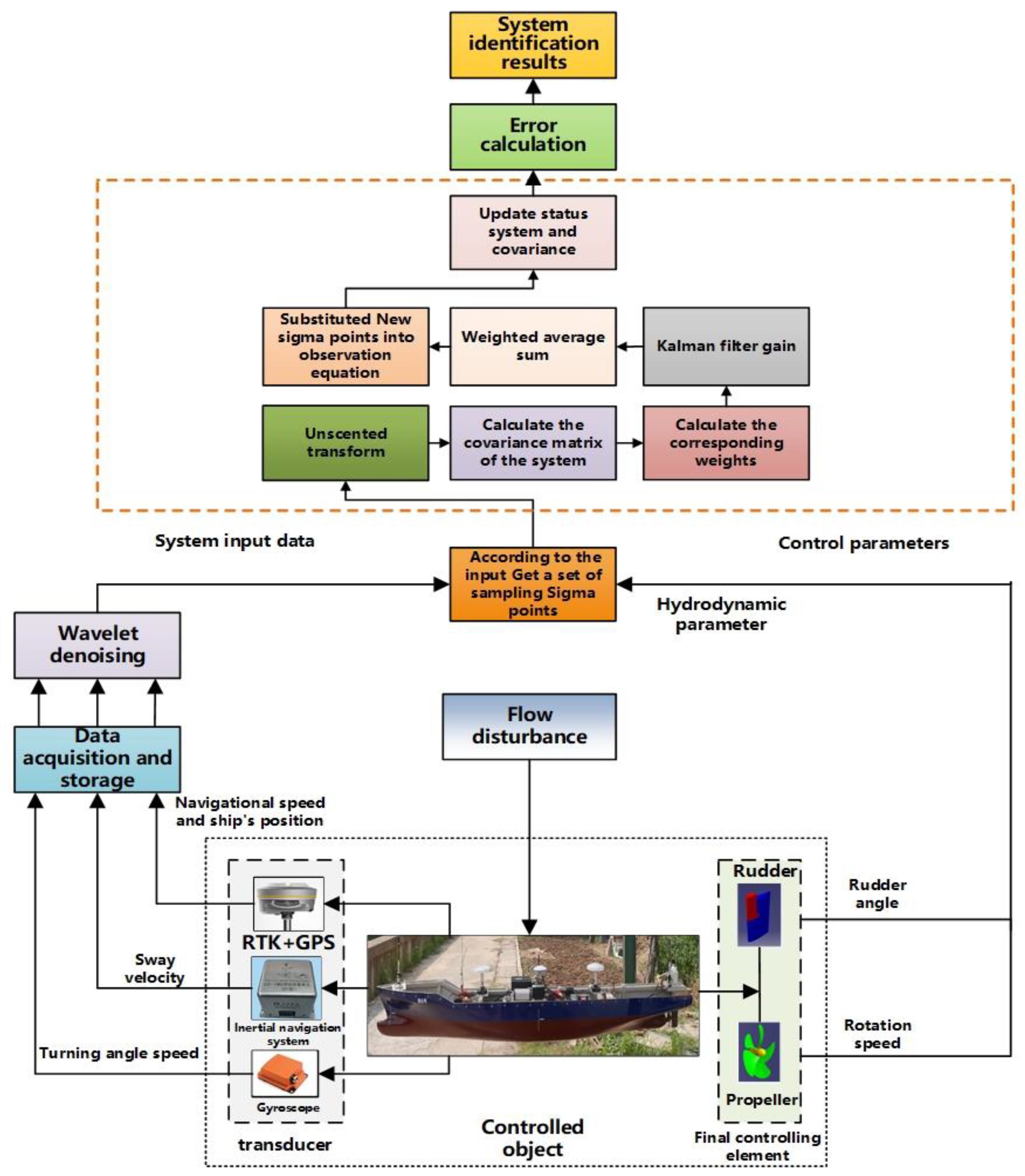
3.1. Online Identification Framework Design

This section describes the idea of modeling and experimentation and describes the method of using a UKF to make identifications from a macro level. Figure 2 shows the idea of the algorithm and the operating principle of the experiment.
First, the state and control quantities collected by the ship’s various equipment are taken as the input. Second, after rolling denoising, the state and control quantities are used in UKF to identify the model parameters. Finally, after calculating the corresponding error, the identification result is output. To improve the stability of the identification results, this research adopts a sliding time window method for data input. t is taken as the window length, time k is taken as the real sampling time, time k − i is taken as the median sampling time, the sliding time window can be traced back to k − 2i moment and the average value of the entire interval is used for judgment. At time k, the estimated values of the system output parameters are the identification result at the moment of k − i. Since the ship motion has a considerable time delay, a relatively short delay will not affect the control effect. A sailing ship will be affected by external disturbances such as wind and water fluctuation and the error factors of the measuring instrument itself, leading to unavoidable errors in the measured data. The time sever curves’ continuity and smoothness of 𝑢, 𝑣 and 𝑟 are poor, affecting the identification accuracy to a certain extent. To solve this problem, wavelet analysis and a sliding time window are combined in this study to carry out real-time denoising of the 𝑢, 𝑣 and 𝑟 values obtained from the experiment [12]. Then, the identification results of the denoising and original data are compared as system inputs in the self-navigation experiment. We first extract the features of the input sequence and then use low-pass filtering to reconstruct the collected feature signals. The signal with noise is decomposed into wavelet decomposition coefficients and compared with a set threshold value. The coefficients that are less than the threshold values are removed, and the remaining coefficients are transformed using an inverse wavelet transform. Finally, we obtain the denoised signal.
We carry out two-layer denoising for the wavelet and synchronize the wavelet analysis with the filter. In Figure 3, p + 1 sampling time is taken as the base point. For each sampling time, denoising is carried out for the first p time, and the parameter value after denoising at this time is taken as the input value of filtering to achieve the effect of synchronous rolling with the filter. We compared the identification results with wavelet denoising and determined whether the identification accuracy of the output parameters was improved by rolling denoising. After wavelet denoising, the smoothness and continuity of the curves were obviously improved.

3.2. Application of the UKF Algorithm

An unscented Kalman filter adopts the framework of a linear Kalman filter and uses the unscented transform (UT) to address the nonlinear transmission problem of the mean and covariance of the parameters to be estimated without linearizing a nonlinear model [16]. This overcomes the problem of linearization error that is inevitably introduced in Taylor’s expansion of a nonlinear model by an EKF algorithm. The method of unscented transformation takes several sampling points in the original state distribution and assigns some weight so that the mean and covariance of these sampling points are equal to the mean and covariance of the original state distribution (that is, to obtain a probability density distribution similar to the original state distribution), replacing the nonlinear system. The specific algorithm principle is described as follows.
Take a nonlinear system 𝑦 = 𝑓(𝑥). The state vector 𝑥 is an 𝑛-dimensional random variable and its mean value 𝑥 and variance 𝑃 are known. Then, 2𝑛 + 1 sampling points 𝑋 and corresponding weights 𝜔 can be obtained using an unscented transformation to calculate the statistical characteristics of y.
(1) Calculate 2𝑛 + 1 sampling points, also called sigma point sets:
{ X ( 0 ) = X ¯ , i = 0 X ( i ) = X ¯ + ( ( n + λ ) P ) i , i = 1 n X ( i ) = X ¯ ( ( n + λ ) P ) i , i = n + 1 2 n ,
where   ( P ) T ( P )   = 𝑃. ( P ) i represents column 𝑖 of the root of the matrix. The first sigma point X to (0) is the mean of the inputs.
(2) Calculate the corresponding weights of these sampling points.
{ ω m ( 0 ) = λ n + λ ω c ( 0 ) = λ n + λ + ( 1 α 2 + β ) ω m ( i ) = ω c ( i ) = 1 2 ( n + λ ) , i = 1 2 n ,
In the above formula, 𝜔𝑚 and 𝜔𝑐 represent the weight of the mean value and the weight of the covariance, respectively, and their superscript represents the sampling time point.
λ = α 2 ( n + κ ) n ,
Parameter 𝜆 is a scaling parameter, scaling factor 𝛼 controls the distribution status of sampling points and a typical value for 𝛼 is in the range of 10−4 to 1. 𝜅 denoted regulatory factor, which typically ensures that matrix (𝑛 + 𝜆) is a semi-positive definite matrix. A larger 𝜅 will choose sigma points far from the mean, whereas a smaller 𝜅 will choose points close to the mean. The optional parameter 𝛽 ≥ 0 is a nonnegative weight coefficient, and its function combines the dynamic differences of higher-order terms in the equation so that the influence of higher-order terms can be taken into account. The unscented transformation is the core of the algorithm. Given a set of sigma points and a transfer function, we need to calculate the new mean and covariance of sigma points so that the new positions of the sigma points are continuously obtained by calculating nonlinear function covariance and the mean of sigma points.
{ X ¯ = i ω m ( i ) X i λ = i ω m ( i ) ( X i X ¯ ) ( X i X ¯ ) T ,
When a Kalman filter is used for system identification and parameter estimation, the general method is to replace the system state quantity in the state matrix with the parameter to be estimated. An observation array is composed of all known quantities that can be measured. Therefore, in this study, the system identification is as follows: in the study of system state matrix X = [X1, X2,..., X9] 𝑇, the parameters in the observation matrix are the ship exercise parameters and coordinates, namely, 𝑍 = [𝑋 𝑌, 𝑢, 𝑣, φ , 𝑟] 𝑇. Noise 𝑊 and 𝑉 are assumed to be Gaussian white noise with a mean of 0 and variance of 1 × 10⁻⁴. In the algorithm, we need to input state transition matrix 𝐹 as the causal relationship between the times before and after the process of data prediction. At the same time, the values of the system parameters estimated at each moment are independent of each other. Therefore, the state transition matrix 𝐹 is set as a unit matrix, where 𝐹 = 𝑑𝑖𝑎𝑔 (1,1,1,1,1,1,1,1,1). Only the influence of external noise interference and observation amount on the estimated parameters is considered. Considering a nonlinear ship system equation of Gaussian white noise, to explain the identification process of UKF more clearly, we introduce the state transition process of the observation matrix in detail based on the ship’s motion model. In this section, we take the ship motion system model as the transformation object, and the following is a description of the transformation process of the observation equation of the ship’s motion system.
First, we solve the first derivative of the ship’s motion parameters and coordinates.
Z ˙ = [ x ˙ y ˙ u ˙ v ˙ φ ˙ r ˙ ] = [ u c o s ( φ ) v s i n ( φ ) u s i n ( φ ) + v c o s ( φ ) m 22 m 11 v r X u + X u | u | | u | m 11 u + τ u m 11 m 11 m 22 u r Y v + Y v | v | | v | m 22 v r m 11 m 22 m 33 u v N r + N r | r | | r | m 33 r + τ r m 33 ] ,
Second, the observation matrix is differentiated.
X k + 1 = X k + t k t k + 1 [ x ˙ ( t ) y ˙ ( t ) u ˙ ( t ) v ˙ ( t ) φ ˙ ( t ) r ˙ ( t ) ] d t ,
Then, the differential equation of the state transition is further expanded.
x k + 1 = x k + [ u k t k t k + 1 cos ( φ k + φ ˙ k · ( t t k ) ) d t v k t k t k + 1 sin ( φ k + φ ˙ k · ( t t k ) ) d t u k t k t k + 1 sin ( φ k + φ ˙ k · ( t t k ) ) d t + v k t k t k + 1 cos ( φ k + φ ˙ k · ( t t k ) ) d t v k r k m 22 m 11 t u k | u | k X u + X u | u | m 11 t + τ u · k 1 m 11 t u k r k t v k | v | k Y v + Y v | v | m 22 t r t + φ k u k v k m 11 m 22 m 33 t r k | r | k N r + N r | r | m 33 t + τ r · k 1 m 11 t ] ,
The following integral equation is solved.
x k + 1 = x k + [ u k φ k ˙ ( sin ( φ k + φ ˙ k t ) sin ( φ k ) ) + v k φ ˙ k ( cos ( φ k + φ ˙ k t ) cos ( φ k ) ) u k φ k ˙ ( cos ( φ k + φ ˙ k t ) + cos ( φ k ) ) + v k φ ˙ k ( sin ( φ k + φ ˙ k t ) sin ( φ k ) ) v k r k m 22 m 11 t u k | u | k X u + X u | u | m 11 t + τ u · k 1 m 11 t u k r k t v k | v | k Y v + Y v | v | m 22 t r t + φ k u k v k m 11 m 22 m 33 t r k | r | k N r + N r | r | m 33 t + τ r · k 1 m 11 t ] ,
Then, we provide the noise equation V(k) for Z(k).
V ( k ) = [ V a , k V t , k ] ,
The noise matrix at the position is described as follows.
V a , k ~ N ( 0 , σ a 2 ) ,
The angle and velocity noise matrix is described as follows.
V ~ N ( 0 , σ r ˙ 2 ) ,
After adding the noise matrix, the complete ship identification model is described as follows.
x k + 1 = x k + [ u k φ k ˙ ( sin ( φ k + φ ˙ k t ) sin ( φ k ) ) + v k φ ˙ k ( cos ( φ k + φ ˙ k t ) cos ( φ k ) ) u k φ k ˙ ( cos ( φ k + φ ˙ k t ) + cos ( φ k ) ) + v k φ ˙ k ( sin ( φ k + φ ˙ k t ) sin ( φ k ) ) v k r k m 22 m 11 t u k | u | k X u + X u | u | m 11 t + τ u · k 1 m 11 t u k r k t v k | v | k Y v + Y v | v | m 22 t r t + φ k u k v k m 11 m 22 m 33 t r k | r | k N r + N r | r | m 33 t + τ r · k 1 m 11 t ] + [ 1 2 ( t ) 2 V a , k cos ( φ ) 1 2 ( t ) 2 V a , k sin ( φ ) 1 2 ( t ) 2 · V a , k 1 2 ( t ) 2 · V a , k 1 2 ( t ) 2 · V r ˙ , k 1 2 ( t ) 2 · V r ˙ , k ] ,
Using the above matrix setting, the nonlinear ship motion model is arranged into the state space form specified by the Kalman filter algorithm. After setting the state space, the following work was performed to find the state of the system: that is, to estimate the minimum variance of the parameters to be estimated. This work is achieved by using the recursive formula of the Kalman filter.
The following state space is used to represent a nonlinear system:
{ X ( k + 1 ) = f ( X ( k ) , W ( k ) ) Z ( k ) = h ( X ( k ) , V ( k ) ) ,
where 𝑘 is a discrete-time point and 𝑓 is the state transition function. h is the observation function; 𝑊 and 𝑉 are system noise and observation noise, respectively, and their variances are 𝑄 and 𝑅, respectively.
Based on the principle of unscented transformation and the above nonlinear state space, the basic steps of the UKF algorithm are as follows:
  • Obtain a set of sampling points and their corresponding weights using Formulas (2) and (3).
X ( i ) ( k | k ) = [ X ^ ( k | k ) X ^ ( k | k ) + ( n + λ ) P ( k | k ) X ^ ( k | k ) ( n + λ ) P ( k | k ) ] ,
ω ( i ) ( k | k ) = [ λ n + λ 1 2 ( n + λ ) ] ,
2.
Calculate the one-step prediction of the 2𝑛 + 1 sampling points, 𝑖 = 1,2... 𝑛 + 1,2.
X ( i ) ( k + 1 | k ) = f [ k , X ( i ) ( k | k ) ] ,
3.
Calculate the one-step prediction and covariance matrix of the system state obtained from the weighted sum of the predicted values of the sigma point set.
X ^ ( k + 1 | k ) = i = 0 2 n ω m ( i ) X ( i ) ( k + 1 | k ) ,
P ( k + 1 | k ) = i = 0 2 n ω m ( i ) [ X ^ ( k + 1 | k ) X ( i ) ( k + 1 | k ) ] [ X ^ ( k + 1 | k ) X ( i ) ( k + 1 | k ) ] T + Q   ,
4.
According to the one-step predicted value of the system state, an unscented transformation is used again to generate a new set of sigma points.
X ( i ) ( k + 1 | k ) = [ X ^ ( k + 1 | k )     X ^ ( k + 1 | k ) + ( n + λ ) P ( k | k )   X ^ ( k + 1 | k ) ( n + λ ) P ( k | k ) ,
5.
By substituting the new set of sigma points into the observation equation, the one-step predicted value of the observed quantity can be obtained, 𝑖 = 1,2... 2𝑛 + 1.
Z ( i ) ( k + 1 | k ) = h [ k , X ( i ) ( k + 1 | k ) ] ,
6.
By summing the one-step prediction observation value of the sigma point set, the one-step prediction means, covariance and one-step prediction covariance of the system state are obtained.
Z ¯ ( k + 1 | k ) = i = 0 2 n ω m ( i ) Z ( i ) ( k + 1 | k ) ,
P Z k Z k = i = 0 2 n ω c ( i ) [ Z ( i ) ( k + 1 | k ) Z ¯ ( k + 1 | k ) ] [ Z ( i ) ( k + 1 | k ) Z ¯ ( k + 1 | k ) ] T + R ,
P X k Z k = i = 0 2 n ω c ( i ) [ X ( i ) ( k + 1 | k ) Z ¯ ( k + 1 | k ) ] [ Z ( i ) ( k + 1 | k ) Z ¯ ( k + 1 | k ) ] T ,
7.
Calculate Kalman filter gain.
K ( k + 1 ) = P X k Z k P X k Z k 1 ,
8.
Finally, the state and covariance update of the system are calculated.
X ^ ( k + 1 | k + 1 ) = X ^ ( k + 1 | k ) + K ( k + 1 ) [ Z ( k + 1 ) Z ^ ( k + 1 | k ) ] ,
P ( k + 1 | k + 1 ) = P ( k + 1 | k ) K ( k + 1 ) P Z k Z k K T ( k + 1 ) ,
It can be seen that the state probability density function obtained using the UT approximation is a statistical approximation rather than a solution. At the end of this section, the flow of the UKF algorithm is shown in Algorithm 1:
Algorithm 1 Unscented Kalman filter identification algorithm.
Principle of the UKF Online Identification Algorithm
1: Set the sampling rule of sigma points
2: Set the weight of sampling points
3: Set the original initial value of the parameters
4: Obtain the initial filter value
5: for i = 1:𝑛
6: Set state space 𝑋(𝑘) 𝑍(𝑘)
7: Enter the ship movement parameters 𝑢, 𝑣, 𝑟, τ u and τ r
8: Sliding time window (1)
9: Unscented Kalman filter (1)
10: Wavelet denoising
11: Sliding time window (2)
12: Unscented Kalman filter (2)
13: end
14: Calculated identification error
τ u and τ r are the longitudinal torque of the propeller and the steering torque of the rudder in the x-direction, respectively. The expressions for these two parameters are as follows:
τ u = η 0 K T ρ D 4 n 2 ,
τ r = 3.9 L A R V s 2 sin 2 σ ,
where K T is the thrust coefficient, η 0 is the interaction coefficient between the propeller and the hull, D is the propeller diameter, σ is the rudder angle, n is the propeller speed, A R is the rudder area, V s is the shipping speed and L is the total length of the ship.

4. Experiment Description

4.1. Free-Running Test Platform and Design

The function of the test platform is to control the ship model and carry out the corresponding movement according to the long-range control instructions input by a shore machine. In this process, the relevant instruments on the ship model obtained the ship motion data and used wireless transmission equipment to transmit with the purpose of obtaining the initial ship model’s motion state and parameters. The main components are a central control communication system, propeller, steering gear, power supply, gyroscope, inertial navigation system, GPS, wireless antenna and transmission equipment [17]. To ensure the authority and effectiveness of the test results, the ship model in this test is based on the Korea Research Institute of Ships and Ocean Engineering Container Ship (KCS) of the SIMMAN 2008 standard built to a scale ratio of 1:75.5 [18]. The material of the test hull is glass fiber-reinforced plastic, the material of the test appendage is aluminum alloy, the rudder is a balance and suspension rudder, its section is NACA0018 and the material of the propeller model is copper. The overall scales of the ship model and related scale of the propeller and rudder are shown in Table 1. The model’s entity and experimental platform system are shown in Figure 4 and Figure 5, respectively.
In this experimental design, the speed of the test ship was set to 1.1 m/s, the sampling interval was 0.1 s and the total sampling time was 57.5 s. Z-shaped steering tests of ±10°, ±15° and ±20° were carried out, and the right 20° Z-shaped steering test was finally selected as the system’s input data for identification. At the beginning of the long-range control ship model steering test, a shore machine records the relevant parameters and online identification until the test is completed. Then, we compared the collected data with the navigation identification results.

4.2. Contrasting Experiments before and after Denoising

Based on Zheng’s experimental results, the UKF and EKF algorithms were compared to highlight the difference between the two algorithms [12]. Similarly to the EKF identification process, two sets of initial filtering values should be set first. The debugged initial values of the EKF are directly used here.
𝑋original = [100; 300; 100; 7.7; 7.7316; −158; −161.5477; −437; −438.4421],
𝑋denoising = [100; 300; 100; −13; −13.1252; 837; 844.9488; −136; −136.3903],
The covariance matrix of parameters is also set as the unit matrix.
𝑃𝑈𝐾𝐹 = 𝑑𝑖𝑎𝑔 [1,1,1,1,1,1,1,1,1],
Unlike EKF, some parameters in the untraced transform should also be preset. According to some research examples, the values are 𝛼 = 1; 𝛽 = 2; 𝜅 = 1. Second, both simulation experiments are carried out online, and the data were collected and updated in real time. The motion parameters and coordinate track identification results obtained based on the original results, and denoised data are shown in Figure 6 and Figure 7, respectively.
As shown in Figure 6, when UKF is used for identification, the accuracy of the identification results obtained based on the denoised data is higher than that based on the original data, which is consistent with the KF and EKF. Therefore, the following conclusions can be drawn: real-time denoising of ship motion data using wavelet analysis can effectively reduce the interference of the external environment on identification results and improve the identification accuracy of hydrodynamic derivatives. By comparing the identification results of the three algorithms, it can be seen that UKF has the best fitting time curve for each motion parameter, and the identification error is the smallest among the three algorithms. The hydrodynamic derivative identification results obtained from the two groups of tests are shown in Figure 8 and Figure 9.
Figure 8 and Figure 9 show that the hydrodynamic derivative identification results obtained based on the denoised data have better convergence, a faster convergence rate and are more stable.

4.3. Comparison of the Identification Effects to Other Algorithms

To prove the accuracy of the Kalman filter in identifying the ship’s motion system, we use the Ordinary Least Squares (OLS) algorithm to identify the system based on the same self-navigation model test data and ship motion model as a comparison of the three Kalman filter algorithms [19]. After obtaining the identification results of the least squares method and linear Kalman filter, they are compared with each Kalman filter. The time curves of each parameter are shown in Figure 10. As demonstrated above, denoising the ship motion data can effectively improve identification accuracies. This study only compares identification results obtained by each algorithm based on the denoised data.
In the experiment of the last stage, we adopted an EKF, KF and the least squares algorithms and compared the corresponding identification results. On this basis, we added the result of the UKF algorithm and conducted the following analysis. First, we set the starting point as (−19.5, 8). The trajectory can be seen from Figure 9, and there is no significant difference in the fitting of the coordinate track in the first half, but at the end, the OLS algorithm showed an apparent deviation trend compared with other algorithms, and the KF algorithm slightly deviated from reference, while UKF maintains a high fitting degree with the actual ship track at the end. Second, it can be seen from the change curves of 𝑢, 𝑣 and 𝑟 that the KF’s fitting of the ship motion parameters is poor, especially at the data turning point and peak value. Finally, although EKF follows well most of the time, it sometimes fluctuates, and its identification stability is weaker than that of UKF.
To compare and evaluate the identification effects of several algorithms, the root mean square error (RMSE) and distance between two points are introduced to calculate the estimation error and coordinate track errors of 𝑢, 𝑣 and 𝑟 [20]. The RMSE calculation formula is as follows.
RMSE = 1 n i = 1 n ( y ^ i y i ) 2 ,
In this online identification experiment, y ^ i indicates the estimated value of 𝑢, the disk and the disk at 𝑖 (that is, the filter value). y i indicates the actual values of 𝑢, 𝑣 and r at 𝑖. The error table of the above identification tests is shown in Table 2.
By comparing the denoised data of each method with the original data, we found that, on the one hand, the parameter estimation error of each algorithm is reduced to a certain extent, especially the identification error of the coordinate track, which is significantly reduced after the wavelet denoising of the ship’s motion data collected in the experiment. By observing the difference between the denoised data and the original data, we can also determine that denoised data will produce specific errors according to different methods. Among them, the UKF’s denoising conditions are optimal in four cases. On the other hand, in terms of the identification error of the motion parameters, UKF has the highest identification accuracy, followed by EKF, KF and OLS, which have low identification accuracy, but system identification has also been successfully carried out. It can be seen that the UKF method is superior in system identification, which proves its feasibility and accuracy in ship motion system identification.

5. Conclusions

In this paper, UKF is used as a tool, a rolling identification framework is built and the parameters of a ship motion system are identified online through a free self-navigation experiment. The combination of wavelet denoising and a sliding time window allows identification to reach an online rolling state. In addition, the identification results show that the online identification accuracy of the nonlinear ship motion system based on UKF is higher than that of other Kalman filtering algorithms. It more effectively solves the time-varying problem of ship parameters in sailing and indirectly improves the safety and economy of ship sailing by improving the identification accuracy. It provides essential services for the future intelligent navigation control of ships.

Author Contributions

Conceptualization, J.Z. and Y.L.; methodology, J.Z. and M.Y.; software, M.Y. and D.Y.; validation, M.Y.; formal analysis, D.Y. and M.Y.; investigation, J.Z. and Y.L.; resources, J.Z. and Y.L.; data curation, J.Z., M.Y. and Y.L.; writing—original draft preparation, M.Y. and D.Y.; writing—review and editing, J.Z. and Y.L.; visualization, D.Y.; supervision, J.Z., Y.L. and Y.Z.; project administration, J.Z. and Y.L.; funding acquisition, J.Z. and Y.L. All authors have read and agreed to the published version of the manuscript.

Funding

This research was funded by Nation Nature Science Foundation of China, grant number 51709166 and 51909155; the Scientific Research Program of Shanghai Science and Technology Commission, grant number 21692193000 and 22010501800.

Institutional Review Board Statement

Not applicable.

Informed Consent Statement

Not applicable.

Data Availability Statement

Please refer to “An online identification approach for a nonlinear ship motion model based on a receding horizon” in section “EKF identification results” at https://journals.sagepub.com/doi/10.1177/01423312211019654 (accessed on 1 March 2022).

Conflicts of Interest

The authors declare no conflict of interest.

References

  1. Luo, W.; Soares, C.G.; Zou, Z. Parameter Identification of Ship Maneuvering Model Based on Support Vector Machines and Particle Swarm Optimization. J. Offshore Mech. Arct. Eng. 2016, 138, 031101. [Google Scholar] [CrossRef]
  2. Luo, W.L.; Zou, Z.J. Identification of Response Models of Ship Maneuvering Motion Using Support Vector Machines. J. Ship Mech. 2007, 11, 832–838. [Google Scholar]
  3. Zhang, X.G.; Zou, Z.J. Black-box modeling of vessel manoeuvring motion based on feed-forward neural network with Chebyshev orthogonal basis function. J. Mar. Sci. Technol. 2013, 18, 42–49. [Google Scholar] [CrossRef]
  4. Wang, X.-G.; Zou, Z.-J.; Hou, X.-R. System identification modelling of vessel manoeuvring motion based on epsilon—Support vector regression. J. Hydrodyn. 2015, 27, 502–512. [Google Scholar] [CrossRef]
  5. Xue, Y.; Liu, Y.; Ji, C.; Xue, G.; Huang, S. System identification of ship dynamic model based on Gaussian process regression with input noise. Ocean. Eng. 2020, 216, 107862. [Google Scholar] [CrossRef]
  6. Wang, N.; Dong, N.; Liu, Y.; Han, M. Vessel maneuvering model identification using multi-output dynamic fuzzy neural networks. In Proceedings of the 33rd Chinese Control Conference, Nanjing, China, 28–30 July 2014; pp. 5144–5149. [Google Scholar] [CrossRef]
  7. Moreira, L.; Soares, C.G. Dynamic model of manoeuvrability using recursive neural networks. Ocean. Eng. 2003, 30, 1669–1697. [Google Scholar] [CrossRef]
  8. Yin, J.; Wang, N.; Perakis, A.N. A Real-Time Sequential Ship Roll Prediction Scheme Based on Adaptive Sliding Data Window. IEEE Trans. Syst. Man Cybern. Syst. 2018, 48, 2115–2125. [Google Scholar] [CrossRef]
  9. Huang, B.G.; Zou, Z.J.; Ding, W.W. Online prediction of ship roll motion based on a coarse and fine tuning fixed grid wavelet network. Ocean. Eng. 2018, 160, 425–437. [Google Scholar] [CrossRef]
  10. Yoon, H.K.; Rhee, K.P. Identification of hydrodynamic coefficients in vessel maneuvering equations of motion by Estimation-Before-Modeling technique. Ocean. Eng. 2003, 30, 2379–2404. [Google Scholar] [CrossRef]
  11. Deng, F.; Levi, C.; Yin, H.; Duan, M. Identification of an Autonomous Underwater Vehicle hydrodynamic model using three Kalman filters. Ocean. Eng. 2021, 229, 108962. [Google Scholar] [CrossRef]
  12. Zheng, J.; Yan, M.; Li, Y.; Huang, C.; Ma, Y.; Meng, F. An online identification approach for a nonlinear ship motion model based on a receding horizon. Trans. Inst. Meas. Control. 2021, 43, 3000–3012. [Google Scholar] [CrossRef]
  13. Perera, L.P.; Oliveira, P.; Guedes Soares, C. Dynamic parameter estimation of a nonlinear vessel steering model for ocean navigation. In Proceedings of the 30th International Conference on Ocean, Offshore and Arctic Engineering, OMAE 2011, Rotterdam, The Netherlands, 19–24 June 2011. OMAE 2011-50249. [Google Scholar]
  14. Skjetne, R.; Smogeli, Y.; Fossen, T.I. Modeling, identification, and adaptive maneuvering of CyberShip II: A complete design with experiments. IFAC Proc. Vol. 2004, 37, 203–208. [Google Scholar] [CrossRef]
  15. Cui, R.; Ge, S.S.; How, B.V.E.; Choo, Y.S. Leader–follower formation control of underactuated autonomous underwater vehicles. Ocean. Eng. 2010, 37, 1491–1502. [Google Scholar] [CrossRef]
  16. Chang, L.; Hu, B.; Li, A.; Qin, F. Transformed Unscented Kalman Filter. IEEE Trans. Autom. Control. 2013, 58, 252–257. [Google Scholar] [CrossRef]
  17. Yuan, X.; Zhang, D.; Zhang, J.; Zhang, M.; Soares, C.G. A novel real-time collision risk awareness method based on velocity obstacle considering uncertainties in ship dynamics. Ocean. Eng. 2020, 220, 108436. [Google Scholar] [CrossRef]
  18. Islam, H.; Soares, C.G. Estimation of hydrodynamic derivatives of a container ship using PMM simulation in OpenFOAM. Ocean. Eng. 2018, 164, 414–425. [Google Scholar] [CrossRef]
  19. Zhang, G.; Zhang, X.; Pang, H. Multi-innovation auto-constructed least squares identification for 4 DOF ship manoeuvring modelling with full-scale trial data. Isa Trans. 2015, 58, 186–195. [Google Scholar] [CrossRef] [PubMed]
  20. Bo, C.; Zhang, S.; Wang, Z.; Lu, A. Research on the Modeling Method Based on Sliding Time Window for Support Vector Machine Soft-Sensing. Process Autom. Instrum. 2006, 027, 45–48. [Google Scholar]
Figure 1. Ship’s 6-DOF motion model.
Machines 10 00312 g001
Figure 2. Principle of the self-propelled model test and online identification.
Machines 10 00312 g002
Figure 3. Schematic diagram of rolling sampling.
Machines 10 00312 g003
Figure 4. Schematic diagram of the free self-propelled model test platform system.
Machines 10 00312 g004
Figure 5. Objective view of the physical model.
Machines 10 00312 g005
Figure 6. Identification results based on the original data.
Machines 10 00312 g006
Figure 7. Identification results based on the denoised data.
Machines 10 00312 g007
Figure 8. Identification of hydrodynamic derivatives based on the original data.
Machines 10 00312 g008
Figure 9. Identification of hydrodynamic derivatives based on the denoised data.
Machines 10 00312 g009
Figure 10. Comparison diagram of ship identification results using different algorithms.
Machines 10 00312 g010
Table 1. Physical model parameters.
ParametersReal ShipFree-Running Ship
Hull parameter
Lpp (m)230.03.0464
Lwl (m)232.53.0791
Breadth (m)32.20.4265
Depth (m)19.00.2517
Draft (m)10.80.1430
Displacement (m3)52,0300.1209
Longitudinal center on buoyancy (%)−1.48−1.48
Hull surface area without rudder (m2)95301.6719
Block coefficient (Cb)0.6510.651
Midship Section coefficient (CM)0.9850.985
Rudder parameter
S of the rudder (m2)1150.0202
Projected area of rudder side (m2)54.450.0096
Rudder height (m)9.900.1311
Mean chord (m)5.500.0728
Mean thickness (m)0.990.0131
Turning rate (deg/s)2.3220.2
Propeller parameter
TypeKP505KP505
No. of blades55
Diameter (m)7.90.105
Pitch ratio of 0.7R (P/D)0.9970.997
Section lineα = 0.8α = 0.8
Hub ratio0.1800.180
RotationRight handRight hand
Expended Area ratio (AE/A0)0.8000.800
Table 2. The error mean of each algorithm in the entire identification process.
AlgorithmSystem InputSurge Velocity (m/s)Sway Velocity (m/s)Yaw Velocity (m/s)Coordinate Distance (m)
EKFDenoised data0.00320.00490.18520.1122
Original data0.00420.00460.23441.8444
KFDenoised data0.00370.01500.48690.1517
Original data0.00630.01350.55081.5448
OLSDenoised data0.02530.05370.53190.6668
UKFDenoised data0.00240.00360.10420.0850
Original data0.00300.00470.14800.1050
Publisher’s Note: MDPI stays neutral with regard to jurisdictional claims in published maps and institutional affiliations.

