Abstract
This paper deals with the stability characteristics of zeros for sampled-data models with a class of triangle sample and hold realized by a traditional zero-order hold. For any controlled models in the modern industrial system, using a digital control strategy has been shown to provide the means to achieve the assigned objectives. In this process, one must utilize the sample and hold device to obtain the sampled-data models. Previous studies have shown that the triangle sample and hold can improve the stability properties of zeros of a sampled-data control system compared with zero-order hold. However, it is difficult to use triangle sample and hold in practice. In this paper, an approximated method of using triangle sample and hold is proposed. More importantly, on the basis of that method, we explicitly derive the corresponding accurate sampled-data model of controlled models. In addition, we also provide the expression for sampling zeros and the theorem for the stability of a linear control system in the fast sampling process. The results of this paper show that the proposed method has the same advantages as the accurate one. Finally, theoretical findings are validated through numerical simulations with different considerations.
1. Introduction
Since the seminal research paper by Åström, et al. was published in 1984 [1], the zeros of sampled-data model has acquired increasing research interest, as it has been regarded as the fundamental means of analysis before the design of a control strategy [2,3,4,5,6,7]. Simultaneously, the stability of zeros of a controlled system can affect the minimum phase (MP) property. A continuous-time system is in non-minimum phase (NMP) if there exists at least one zero in the right-half plane. Similarly, a discrete time system is in NMP if it has at least one zero outside the unit circle. The control performance cannot be satisfied when the controlled system is non-minimum phase (NMP) [2]. The control design for NMP is challenging. Therefore, checking the zeros’ stability properties of sampled-data model is a vital preliminary work to designing a control strategy [8].
From the previous literature, one can know that the stability of zeros is not naturally preserved when a continuous-time system is discretized by sample and hold [1,9,10]. The mapping relationship of the zeros between the continuous-time system and sampled-data models is complex compared with poles. Zeros of the linear sampled-data model are classified into two categories: intrinsic zeros and sampling zeros [11]. An intrinsic zero is same as the pole of a system, existing as the simple relation: and , where T is the sampling period, and z and p represent the zero and pole of continuous-time system, respectively. However, the sampling zeros of the sampled-data model do not have the above simple relation with the original zeros of the continuous-time system.
NMP properties of a controlled system are the major obstacle to control, but discretization with sample and hold may alleviate the problem. The core idea of this method is assigning zeros to the stable area in the process of obtaining the sampled-data model. Many research works in [5,12,13,14,15] have shown that an NMP continuous-time system may map into an MP discrete time model. In addition, the MP properties of models play an important role in modern control systems, such as networked control systems (NCSs) and cyber-physical systems (CPSs). The models face zero-dynamic attacks (ZDAs) threats when they are NMP (i.e., the unstable zeros arise from in the discretization process) [6,16,17,18,19]. Thus, it is necessary to analyze the properties and stability of the sampling zeros of sampled-data models. As compared with traditional sample and hold forms, such as zero-order hold (ZOH), first-order hold (FOH) and fractional-order hold (FROH) ones, triangle sample and hold (TSH, including backward triangle sample and hold (BTSH) and forward triangle sample and hold (FTSH)) can improve the stability of the zeros of a sampled-data system. What is more, the controlled system will have better performance than with ZOH or FOH [5,20]. The above mentioned results have been clarified theoretically in many papers [5,15,20,21,22,23].
Although the TSHs have a significant advantage in preserving the minimum phase, it is difficult to use the exact TSHs practically. Our previous conference paper studied the properties of sampling zeros in the case of an approximate implementation of BTSH and revealed the advantages of them [24]. However, more research details about the TSH (includes BTSH and FTSH) are not clear. We need to perform more innovative research to reveal the detailed properties of sampling zeros during the TSH approximation implementation. Motivated by putting TSHs into practice, in this paper, we deduce a method of approximating the exact TSH with ZOH. Hence, it is important to investigate the properties of sampling zeros for sampled-data models corresponding to continuous-time systems with TSH-implemented ZOHs. To the best of our knowledge, research about TSH applications in practice using the above method is still missing.
Our goals for this study were to deduce theoretical method realizing the implementation of TSHs in practice, and to present the MP conditions of sampled-data models with approximate TSH. Therefore, the main contribution of this paper is exploring the approximate method for triangle sample and hold. The stability of zeros of the sampled-data model was improved, and even has the same level as the accurate one. The main contents of this paper can be briefly summarized as follows:
The basic idea of the method is shown in Section 2. The problem formulation and some preliminary knowledge are also introduced there. Our main results are presented in Section 3, where the expression of sampling zeros about the corresponding sampled-data system is discussed, as the sampling period is small, and the theorem for the stability of zeros is proved. Numerical simulations are given to demonstrate the effectiveness of the method, alongside the benefits of the proposed method, in Section 4. Finally, the conclusions are given in Section 5.
2. Problem Description and Approximate Triangle Sample and Hold
In this paper, we consider a class of the following nth-order time-invariant single-input and single-output (SISO) system, which is controllable and observable. The sate-space expression is used as follows:
where , and are n-th-order state coefficient matrix and column and row vectors, respectively.
We are interested here in the properties of sampled data models for a continuous time linear system when the input signal is generated by a TSH. Therefore, in this part we give the expressions and approximate methods of BTSH and FTSH.
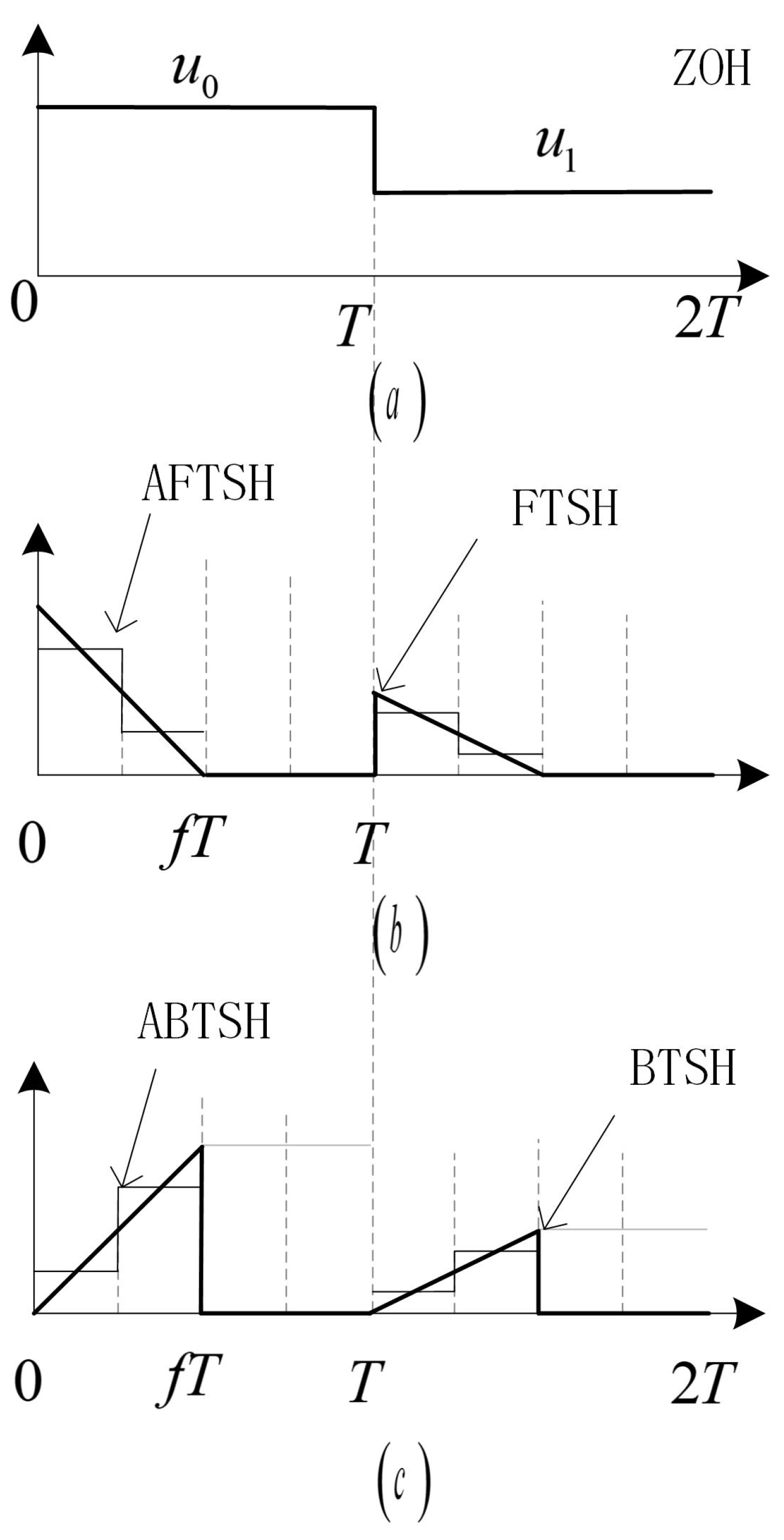
Firstly, using backward triangle sample and hold (BTSH) as the signal reconstruction method, the input function has the following expression [5,20,21], and the structure chart is shown as in Figure 1.
where is the duty cycle of the switched input, ( is the set of natural numbers) and represents the traditional ZOH value in one sampling period.

Figure 1.
The structures of the signal reconstruction outputs of different sample and holds: (a) Zero-order hold. (b) FTSH and approximate FTSH (AFTSH) with . (c) BTSH and approximate BTSH (ABTSH) with [24].
Using the Laplace transform can provide the transfer function of BTSH as
In the approximate realization of TSH process, the core idea of is to use ZOH to generate some step wave in the interval to replace the output values of the original signal. The schematic diagrams of approximate triangle sample and hold (AFTSH) and approximate BTSH when are shown in Figure 1b,c, respectively.
With ABTSH as the signal reconstruction method in the process, then the input function is deduced as follows:
where N represents the number of step waves, and .
Naturally, one can obtain the transfer function of ABTSH by using Laplace transform. It is written as
As the step , we have
Secondly, we analyze the approximate properties of forward triangle sample and hold (FTSH). The schematic diagram of the original FTSH and approximate FTSH are shown in Figure 1, and the input function of the FTSH is denote as .
One can also use the Laplace transform to obtain the transfer function:
Analogously, we also use the ZOH to generate N step waves in the interval to realize the FTSH. Thereafter, using the approximate FTSH as the new signal reconstruction method can be written as
For better knowledge about FTSH and AFTSH, it is necessary to analyze the function of AFTSH in the frequency domain, i.e., using the Laplace transform to obtain the transfer function.
As , we also have
Remark 1.
Remark 2.
From the above approximate method of TSH, obviously the simplest condition is , and the corresponding diagram is shown in Figure 1, giving the following expression.
Next, we recall the definitions of standard Euler–Frobenius polynomials, which play an important role in the deduce process of this paper.
Definition 1.
The Euler–Frobenius polynomials satisfy
where and
Remark 3.
Definition 1 was first presented in [11], and more about the properties of Euler–Frobenius polynomials can be found in [25].
Definition 2 ([3]).
The modified Euler–Frobenius polynomials are defined by
where , and
3. Properties and Stability Conditions of Zeros of Sampled-Data Models
In the above section, we have proved that AFTSH and ABTSH are the operable methods for FTSH and BTSH in practice, respectively. However, the properties of the zeros of sampled-data models using the approximate triangle sample and hold as the signal reconstruction method are not clear. It is an interesting job to explore the properties and the remaining stable conditions of zeros of sampled-data models with AFTSH and ABTSH. In this section, we analyze that topic and give the theoretical results for when the sampling period is sufficiently small.
3.1. Properties of Zeros
In the research process, we followed the ideas from simple to complex, and from special to general. First of all, we will analyze the corresponding results of the integrator control system in the case of approximate TSH.
Theorem 1.
When the controlled system is composed of an rth-integrator with transfer function and the input values are generated by the approximate TSH as the signal reconstruction method, we can obtain the following results.
- (1)
- If ABTSH is the signal reconstruction method, the exact sample-data models of the controlled continuous-time system have the following description of state space.where , and the output of the sampled-data model is . Therefore, the transfer function of the sampled-data model iswhere
- (2)
- If AFTSH is the signal reconstruction method, then the exact sampled-data models of the controlled continuous-time system have the following description of state space.where , and the output of the sampled-data model is . Therefore, the transfer function of the sampled-data model iswhere
Proof of Theorem 1.
Considering the similarity of the two results, here, we only give details of the first result when the input signal of the controlled system is generated by the ABTSH. One can get another result with a simple transformation.
The expression of state space of the r-th integrator control system can be obtained as follows.
where
The output of the system is . From the approximate expression of BTSH in (4), we know that the ABTSH divides interval into N segments. The value is 0 in interval . Therefore, we can obtain the exact expression of sample-data model as follows.
therefore, and ,
Combined with the modified Euler–Frobrnious polynomials (15) and the knowledge in [3], we can show that
Using Cramer’s rule, we can solve for and obtain
where
It is an easy task to compute the determinant of M along the last column. We obtain
Therefore, we can obtain
Noting that the output of sampled-data model is and that the transfer function of sampled-data model is , the result of part 1 of Theorem 1 is obtained.
The proof is complete. □
Remark 4.
In the proofs, the coefficient matrices and of the two results have the same expression.
In addition, the matrix is
which is not a difficult task; refer to the proof process of Theorem 1.
The r-th order integrator system is a special linear control system. It is natural to extend our study to the properties of the zeros of sampled-data models for the general linear control system in the case of approximate TSH.
With the above motivation, we established the following theorem.
Theorem 2.
Let the general linear system with continuous transfer function be the original controlled system. We then have the following results:
- (1)
- (2)
Proof of Theorem 2.
Here we will only give one part of the proof process of the theorem. One can easy obtain the other part based on the proof process. Therefore, the deduced details of the exact sampled-data models of the general continuous-time linear system in the case of ABTSH are given as examples as follows.
The expression of (23) is obtained directly by using the inverse Laplace transform and considering that the transfer function of ABTSH is given by (5).
Suppose that a general continuous-time linear system is a strictly proper nth-order transfer function and the form is written as
where , and is the relative degree of the system.
From the definition of and , we can obtain
Then, based on the definition of the inverse Laplace transform and transformation, the following exact transfer function of the corresponding sampled-data model is obtained.
where , and using , we can simplify the upper equation as
As sampling period , we have that , and
Therefore, the result of (30) can be equivalent to r-th order integrator control system with gain K. Using the same method to deal the integrator system (refer Theorem 1) can obtain the exact sampled-data model as
In addition, for the r-th order integrator control system, using the above computing process and substituting values into (31) appropriately, we finally obtain (24).
Moreover, the proof process of the case of AFTSH is omitted here. It is not a difficult thing to deduce by referring to the above process. □
Remark 5.
From the limit expression of the exact sampled-data model in (24) and (26), we know that the sampled-data model of the strictly proper transfer function with sampled period has n poles converging to and m zeros converging to . More importantly, the remaining zeros (sampling zeros) converge to the roots of and .
3.2. Stability of Zeros
In the above subsection, two important theorems were provided. Here, the properties of zeros of the corresponding sampled-data system are shown in detail. However, it is not intuitive to obtain the stability conditions of the sampling zero of a sampled-data model, and naturally, we give some theoretical results about the sampling zero.
Remark 6 ([3]).
Combined with the Definition 2, we can get some special expressions of the modified Euler–Frobenious polynomial in some case.
Remark 7.
In many practical fields, the relative degree of the control system model is 2; as examples, take a spring-mass-damper oscillator and Chua’s circuit [22,26,27]. We mainly focus on deducing the results of stability conditions of sampled-data models when the relative degree is 1 or 2.
Theorem 3 ([24]).
Suppose that is a strictly proper transfer function with no zeros on the imaginary axis. The approximate BTSH is used as the signal reconstruction model and with a small sampling period. In order to let the control system have the minimum phase, the following condition of the sampled-data model should be satisfied.
Case (i): when the relative degree , for a sufficiently small sampling period, if and only if the original continuous-time system is MP, then the sampled-data system is MP.
Case (ii): when the relative degree , for a sufficiently small sampling period, if f is satisfied with
then the sampled-data system is MP—i.e., the sampling zero of the sampled-data model is always stable.
Theorem 4.
For a strictly proper transfer function with no zeros on the imaginary axis, the approximate FTSH is the signal reconstruction model with a small sampling period. The corresponding sampled-data model is minimum phase should it meet one of the following conditions.
Case (i): when the relative degree , for a sufficiently small sampling period, if and only if the original continuous-time system is MP, then the sampled-data system is also MP.
Case (ii): when the relative degree , for a sufficiently small sampling period, if f is satisfied with
then the sampled-data system is MP; i.e., the sampling zero of the sampled-data model is always stable.
Proof of Theorem 4.
As the zeros of original continuous-time system are stable, for a sufficiently small sampling period, the sampling zeros of sampled-data models with approximate FTSH are the root of . In order to deduce the stable condition of a sampling zero under different relative degrees, we give the following proof process.
Case (i): If the relative degree is , then the . Obviously, the sampled-data model only has an intrinsic zero which exists in the simple mapping relation as between the continuous-time and sampled-data models. Therefore, the resulting sampled-data model is MP if and only if the continuous-time system is MP.
Case (ii): If the relative degree is , from (19), we obtain
In order to reassign the sampling zero located in the unit circle, we need to solve the equation and let the absolute values of roots be less than 1. Then, we have the following conditional expression.
Combined with the limitations of parameter f, if we solve the above equation, we find the feasible solution is . Finally, the theorem’s proof is completed. □
Remark 8.
From the results in Theorems 3 and 4, with the number of step waves , the critical point value of the condition to ensure MP in the case of ABTSH is , which coincides with the results in the case of BTSH [15]. Moreover, for the case of AFTSH, it has the same properties as FTSH in the case of step wave [5].
4. Numerical Example
In this section, an interesting numerical example exemplifies the ideas of this paper. As shown in Theorems 3 and 4, one can find a suitable parameter to ensure the sampled-data system is MP when the BTSH or FTSH is implemented by a ZOH, approximately. Then, we provide the dynamic relationships between the sampling zero and different step waves N or sampling periods T through graphs.
Consider a linear continuous-time system with relative degree 2 and the transfer function
The exact sampled-data model, when an approximate BTSH is used to generate the input signal, can be obtained using the results in Theorem 1 part (1), which yields
where
By direct calculation from (36), one can obtain the exact sampling zero of the sampled-data model located at
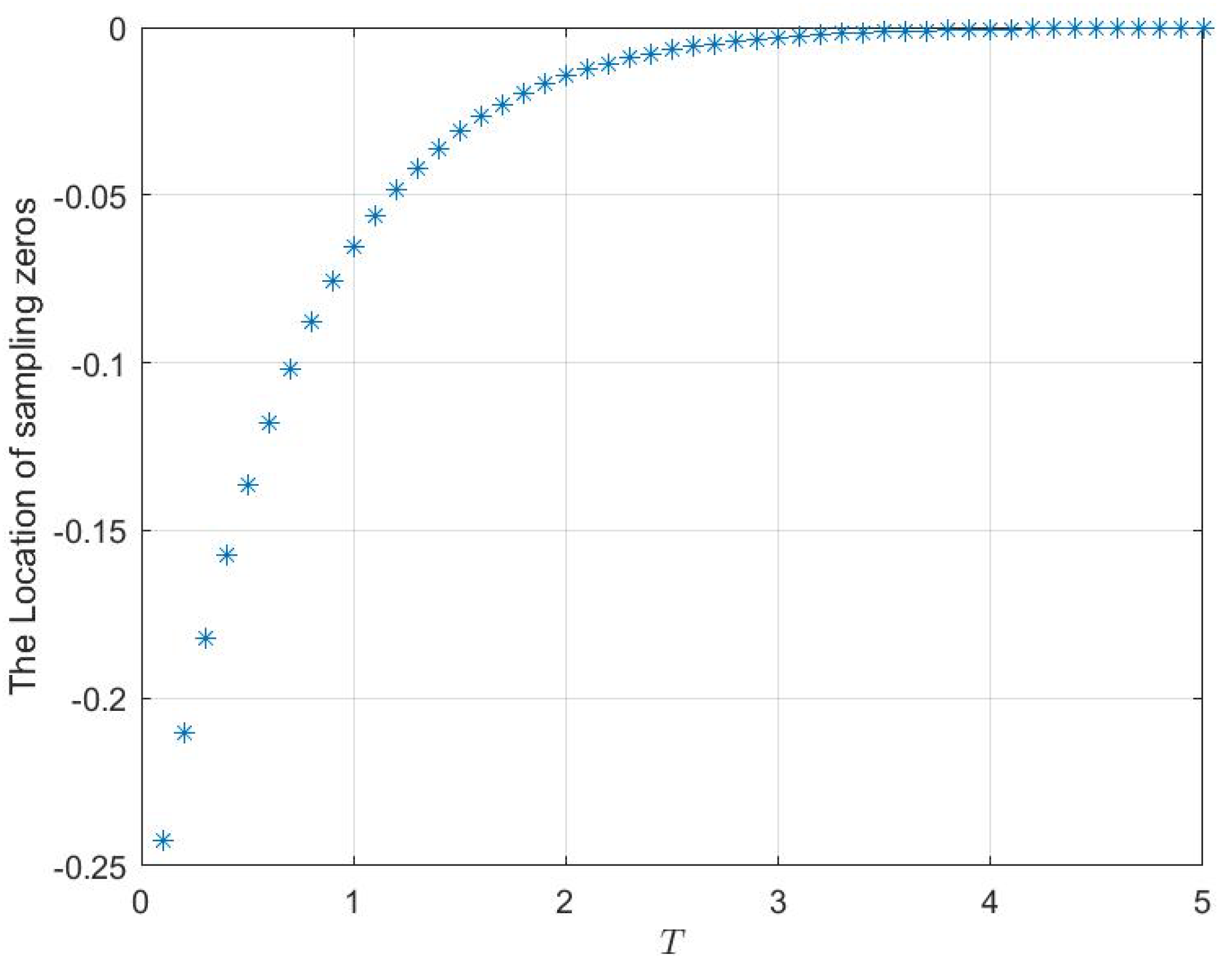
For convenience, from the results in Theorem 3, one can know that f should be satisfied when the step wave is . Therefore, Figure 2 shows different values of sampling zero with respect to sampling period T when we select the variable parameter . Obviously, the sampling zero always be assigned in the unit circle for different sampling period. In other words, the sampled-data model remains minimum phase in the above-mentioned situation.
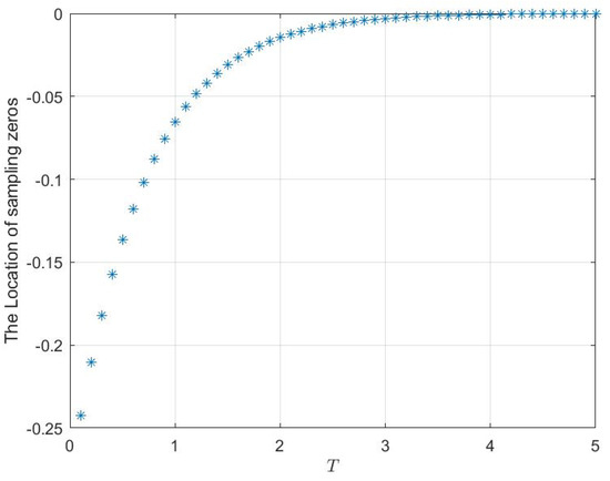
Figure 2.
The asymptotic property of the sampling zero of a sampled-data model with ABTSH in the case of and .
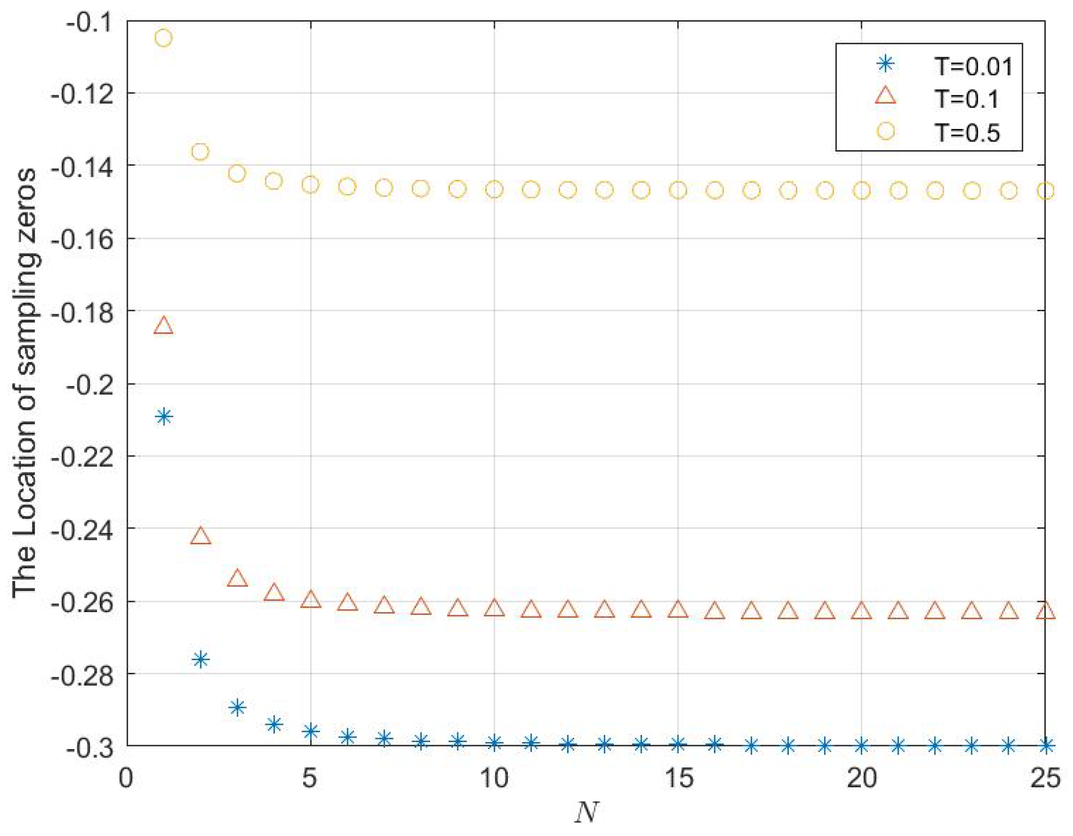
Moreover, from the expression of ABTSH, one can know that the properties of ABTSH are influenced by three parameters: sampling period T, the variable f of BTSH and the number N of step waves. The simulation of Figure 2 is only a special case of sampling zero for fixing N and T.
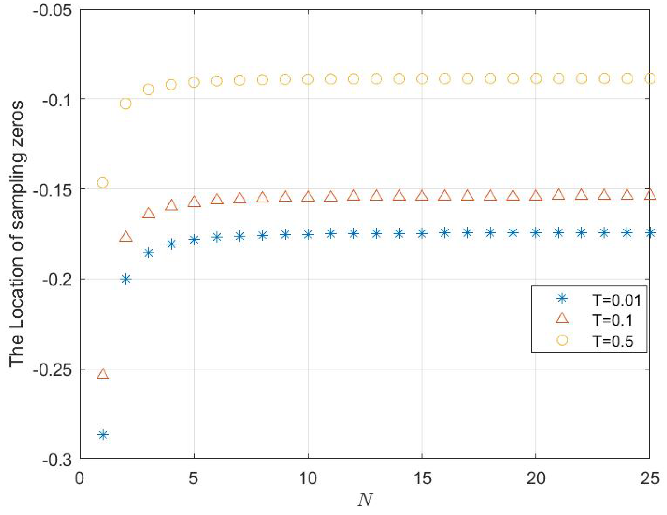
Therefore, it is very significant work to show the asymptotic behavior of a sampling zero when the number of step waves is not fixed. Here, Figure 3 shows the behavior of a sampling zero with different sampling periods, , and , when .
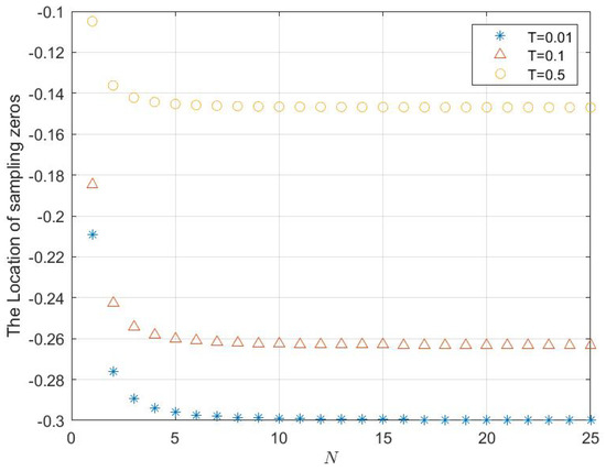
Figure 3.
The different asymptotic properties of the sampling zero of a sampled-data model with different fixed T and not fixed N when using ABTSH with .
On the other hand, if the input signal values are generated by approximate FTSH, then the exact sampled-data model can also be obtained by using the results in Theorem 1 part (2), which yields
where
Therefore, by direct computation from (38), one can also get the exact sampling zero of the sampled-data model located at
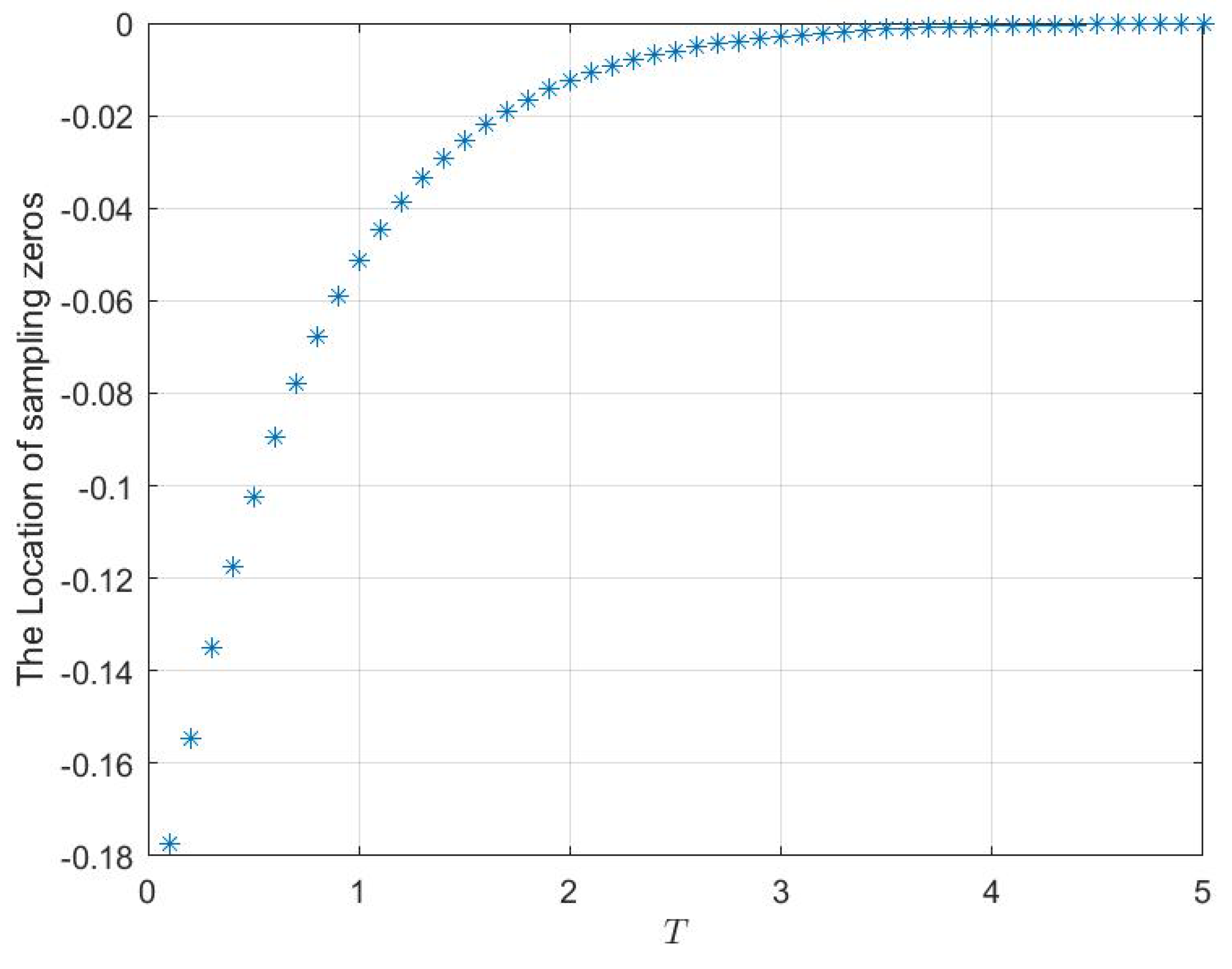
To discuss the properties of the sampling zero in different conditions, we also adopt the same strategy to research the approximate BTSH. Firstly, we select and the step wave . The values of sampling zero with respect to different sampling periods T are shown in Figure 4. Obviously, the sampling zero of the exact sampled-data model in the case of AFTSH can be also assigned in the unit circle for different sampling periods.
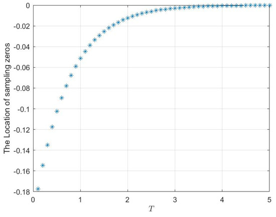
Figure 4.
The asymptotic property of the sampling zero of a sampled-data model using AFTSH in the case of and .
What is more, the location of the sampling zero of exact sampled-data model is also affected by the sampling period T, the variable f of FTSH and the number N of step waves. Here, Figure 5 shows the asymptotic behavior of the sampling zero with different step wave numbers when and sampling period is , or .
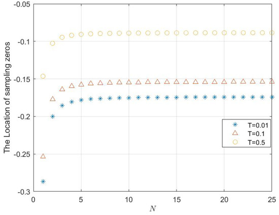
Figure 5.
The different asymptotic properties of the sampling zero of a sampled-data model with different fixed T and not fixed N when AFTSH is used with .
Obviously, for a more general situation of AFTSH, the sampling zero of an exact sampled-data model can also be located in the stable region.
From the results in the simulation diagram of Figure 3 and Figure 5, if the step wave number is fixed, then the distance between the location of the sampling zero and the original point is inversely proportional to the size of the sampling period. This phenomenon reveal a rule which can provide some guidance to select a sampling period in the design process of a digital control strategy.
5. Conclusions
This paper was motivated by the use of the triangle sample and hold devices and proposed one approximate method by using the traditional zero-order hold. We have used theoretical knowledge to reveal the effectiveness of the above implement method. The results have shown the relation between the sampling zero of an exact sampled-data model and the number of step waves in the approximating process. Moreover, the stability conditions of the sampling zero with the relative degrees of an original continuous-time system and step waves were also deduced. Some results of this paper coincide with our previous work [5,15] when the step wave number N is sufficiently large with respect to ABTSH or AFTSH. In addition, we have provided the feasible region about the parameter f, sampling period T and step wave number N to assign the sampling zero of an exact sample-data model located in the unit circle. We have provided the conditions for the stability of sampling zeros when the continuous-time system is sampled by approximate TSH. However, we only gave the results in the case of single-input single-output (SISO) linear system. More needs to be explored, such as the properties of the sampled-data system when the original continuous-time system is nonlinear or time-delayed in the case of approximate TSH; in addition, research about multiple-input multiple-output (MIMO) is also interesting work. In the next study, we will continue to research the latter.
Author Contributions
Conceptualization, M.O. (Minghui Ou), Z.Y. (Zhiyong Yang) and S.L. (Shan Liang); methodology, M.O. (Minghui Ou); software, Z.Y. (Zhiyong Yang) and S.L. (Shuanghong Liu); validation, M.O. (Minghui Ou), Z.Y. (Zhiyong Yang), Z.Y.(Zhenjie Yan), M.O. (Mingkun Ou), S.L. (Shuanghong Liu), S.L. (Shan Liang) and S.L. (Shengjiu Liu); formal analysis, M.O. (Minghui Ou); investigation, M.O. (Minghui Ou) and Z.Y. (Zhiyong Yang); resources, Z.Y. (Zhenjie Yan) and S.L. (Shengjiu Liu); data curation, M.O. (Mingkun Ou); writing—original draft preparation, M.O. (Minghui Ou) and Z.Y. (Zhenjie Yan); writing—review and editing, S.L. (Shan Liang) and S.L. (Shengjiu Liu); visualization, M.O. (Mingkun Ou); supervision, Z.Y. (Zhiyong Yang); project administration, M.O. (Minghui Ou); funding acquisition, M.O. (Minghui Ou) and Z.Y. (Zhiyong Yang). All authors have read and agreed to the published version of the manuscript.
Funding
This research was funded by the National Natural Science Foundation of China (grant number 61771077), the Science and Technology Research Program of Chongqing Municipal Education Commission (grant numbers KJQN202103401, KJQN201903402, KJQN202103404), the Natural Science Foundation of Chongqing, China (grant number cstc2021jcyj-msxmX0532, cstc2018jcyjAX0815) and the Program for Innovation Research Groups at Institutions of Higher Education in Chongqing (grant number CXQT21032).
Institutional Review Board Statement
Not applicable.
Informed Consent Statement
Not applicable.
Data Availability Statement
The data presented in this study are available on request from the corresponding author.
Acknowledgments
We are grateful thanks for the efforts of the conference authors and the ICAMechS working group.
Conflicts of Interest
The authors declare no conflict of interest.
References
- Åström, K.J.; Hagander, P.; Sternby, J. Zeros of sampled systems. Automatica 1984, 20, 31–38. [Google Scholar] [CrossRef]
- Clarke, D.W. Self-tuning control of nonminimum-phase systems. Automatica 1984, 20, 501–517. [Google Scholar] [CrossRef]
- Carrasco, D.S.; Goodwin, G.C.; Yuz, J.I. Modified euler-frobenius polynomials with application to sampled data modelling. IEEE Trans. Autom. Control 2017, 62, 3972–3985. [Google Scholar] [CrossRef]
- Ma, H.; Li, Y.; Xiong, Z. A generalized input-output-based digital sliding-mode control for piezoelectric actuators with non-minimum phase property. Int. J. Control Autom. Syst. 2019, 17, 773–782. [Google Scholar] [CrossRef]
- Ou, M.; Liang, S.; Zhang, H.; Liu, T.; Liang, J. Minimum phase properties of systems with a new signal reconstruction method. IFAC-PapersOnLine 2020, 53, 610–615. [Google Scholar] [CrossRef]
- Kim, D.; Ryu, K.; Back, J. Zero-Dynamics Attack on Wind Turbines and Countermeasures Using Generalized Hold and Generalized Sampler. Appl. Sci. 2021, 11, 1257. [Google Scholar] [CrossRef]
- Ortigueira, M.D.; Machado, J.T. A review of sample and hold systems and design of a new fractional algorithm. Appl. Sci. 2020, 10, 7360. [Google Scholar] [CrossRef]
- Hsu, C.C.; Lu, T.C. Minimum-phase criterion on sampling time for sampled-data interval systems using genetic algorithms. Appl. Soft Comput. 2008, 8, 1670–1679. [Google Scholar] [CrossRef]
- Sánchez, C.; Goodwin, G.C.; Yuz, J.I.; Serón, M.; Carrasco, D. Towards a Simple Sampled-Data Control Law for Stably Invertible Linear Systems. IFAC-PapersOnLine 2020, 53, 4582–4587. [Google Scholar] [CrossRef]
- Barcena, R.; De la Sen, M.; Sagastabeitia, I. Improving the stability properties of the zeros of sampled systems with fractional order hold. IEE Proc.-Control Theory Appl. 2000, 147, 456–464. [Google Scholar] [CrossRef]
- Yuz, J.I.; Goodwin, G.C. On sampled-data models for nonlinear systems. IEEE Trans. Autom. Control 2005, 50, 1477–1489. [Google Scholar] [CrossRef]
- Fu, Y.; Dumont, G.A. Choice of sampling to ensure minimum-phase behaviour. IEEE Trans. Autom. Control 1989, 34, 560–563. [Google Scholar] [CrossRef]
- Hagiwara, T. Analytic study on the intrinsic zeros of sampled-data systems. IEEE Trans. Autom. Control 1996, 41, 261–263. [Google Scholar] [CrossRef] [Green Version]
- Hagiwara, T.; Yuasa, T.; Araki, M. Stability of the limiting zeros of sampled-data systems with zero-and first-order holds. Int. J. Control 1993, 58, 1325–1346. [Google Scholar] [CrossRef]
- Ou, M.; Liang, S.; Zeng, C. Stability of limiting zeros of sampled-data systems with backward triangle sample and hold. Int. J. Control Autom. Syst. 2019, 17, 1935–1944. [Google Scholar] [CrossRef]
- Pasha, S.A.; Ayub, A. Zero-dynamics attacks on networked control systems. J. Process Control 2021, 105, 99–107. [Google Scholar] [CrossRef]
- Teixeira, A.; Shames, I.; Sandberg, H.; Johansson, K.H. Revealing stealthy attacks in control systems. In Proceedings of the 2012 50th Annual Allerton Conference on Communication, Control, and Computing (Allerton), Monticello, IL, USA, 1–5 October 2012; pp. 1806–1813. [Google Scholar]
- Dibaji, S.M.; Pirani, M.; Flamholz, D.B.; Annaswamy, A.M.; Johansson, K.H.; Chakrabortty, A. A systems and control perspective of CPS security. Annu. Rev. Control 2019, 47, 394–411. [Google Scholar] [CrossRef] [Green Version]
- Castillo, O.; Benítez-Pérez, H.; Alvarez-Icaza, L. Novel analysis of sampled-data systems stabilised by a pulsed control signal. Int. J. Control 2021, 94, 2766–2774. [Google Scholar] [CrossRef]
- Wang, Y.; Jafari, R.; Zhu, G.G.; Mukherjee, R. Sample-and-hold inputs for minimum-phase behavior of nonminimum-phase systems. IEEE Trans. Control Syst. Technol. 2016, 24, 2103–2111. [Google Scholar] [CrossRef]
- Ou, M.; Liang, S.; Liu, T.; Zeng, C. A stability condition of zero dynamics of a discrete time systems with backward triangle sample and hold. In Proceedings of the 2017 International Conference on Advanced Mechatronic Systems (ICAMechS), Xiamen, China, 6–9 December 2017; pp. 339–343. [Google Scholar]
- Ou, M.; Liang, S.; Zeng, C. A novel approach to stable zero dynamics of sampled-data models for nonlinear systems in backward triangle sample and hold case. Appl. Math. Comput. 2019, 355, 47–60. [Google Scholar] [CrossRef]
- Ou, M.; Liang, S.; Wu, X.; Yang, Z.; Ran, H. Asymptotic properties of zeros for discrete-time linear systems with backward triangle sampled-and-hold using delta operator. In Proceedings of the 2020 Chinese Automation Congress (CAC), Shanghai, China, 6–8 November 2020; pp. 6741–6746. [Google Scholar]
- Ou, M.; Yang, Z.; Wu, X.; Liang, S.; Ou, M.; Ran, H. Zeros of sampled systems with Backward Triangle Sample and Hold realized by Zero Order Hold. In Proceedings of the 2021 International Conference on Advanced Mechatronic Systems (ICAMechS), Tokyo, Japan, 9–12 December 2021; pp. 151–155. [Google Scholar]
- Yuz, J.I.; Goodwin, G.C. Sampled-Data Models for Linear and Nonlinear Systems; Springer: London, UK, 2014. [Google Scholar]
- Zeng, C.; Liang, S.; Xiang, S. A novel condition for stable nonlinear sampled-data models using higher-order discretized approximations with zero dynamics. ISA Trans. 2017, 68, 73–81. [Google Scholar] [CrossRef] [PubMed]
- Berger, T.; Reis, T. Funnel control via funnel precompensator for minimum phase systems with relative degree two. IEEE Trans. Autom. Control 2017, 63, 2264–2271. [Google Scholar] [CrossRef]
Publisher’s Note: MDPI stays neutral with regard to jurisdictional claims in published maps and institutional affiliations. |
© 2022 by the authors. Licensee MDPI, Basel, Switzerland. This article is an open access article distributed under the terms and conditions of the Creative Commons Attribution (CC BY) license (https://creativecommons.org/licenses/by/4.0/).