Article

General Procedure for Servo-Axis Design in Multi-Degree-of-Freedom Machinery Subject to Mixed Loads

Department of Engineering and Applied Sciences, University of Bergamo, 24044 Dalmine, BG, Italy
*
Author to whom correspondence should be addressed.
Machines 2022, 10(6), 454; https://doi.org/10.3390/machines10060454
Submission received: 10 May 2022 / Revised: 3 June 2022 / Accepted: 5 June 2022 / Published: 8 June 2022
(This article belongs to the Section Machine Design and Theory)

Abstract

:
The motion performances of multi-axis machinery are strongly related to the proper design of the servo axes driving the actuated joints, which must fulfil motion requests in terms of speed and torque for the motion design task. Multi-degree-of-freedom machinery highlights, at the joint level, mixed-load conditions due to high dynamic movements and external working forces. Moreover, such systems have a dynamic coupling between the axes due to their mechanical configuration. This mixed-load condition makes the servo-axes design, whose result is the selection of the couple power drive system and transmission, not a trivial procedure. This paper proposes an extensive theoretical discussion that leads to a general procedure for the direct design of the servo axes of multi-degree-of-freedom machinery subject to a mixed-load condition and dynamic coupling between the mechanical joints. The proposed procedure starts with identifying the loads required on the actuated joints without distinguishing between the different contributions. Then, in a few steps, the methodology leads to the direct choice of the PDS/transmission units through a single graphical representation where the load’s peak, thermal and speed conditions are highlighted, along with the possible PDSs and transmissions. The graphical representation proposed also allows the easy and efficient analysis of the effect of transmission selection on the torque and speed margins. Finally, the paper presents the effectiveness of the proposed procedure, applied to the design of the servo axes of a linear delta robot.

1. Introduction

The servo-axis design of a multi-degree-of-freedom machinery, such as robots, requires the simultaneous selection of two components for each servo axis, the power drive system (PDS) and the transmission, where the PDS includes the complete drive module (CDM) and the motor, as indicated in IEC 61800 standard [1]. The transmission connects each PDS to the mechanical input of the machinery’s correspondent degree of freedom, the joint (high-speed transmission output). The servo axes must fulfill the speeds and torques, as a function of time at the joint level, that the machinery needs to realize the required task.
A multi-degree-of-freedom machinery highlights, at the joint level, mixed-load conditions due to highly dynamic movements and external working forces. Moreover, such systems have a dynamic coupling between the axes due to the mechanical configuration. The resulting mass matrix of the dynamic model is something else altogether diagonal and depends on the position reached by the joints. This physical condition shows that the mass seen by each axis is not constant. This mixed load condition makes servo-axes design not a trivial procedure.
The literature shows several papers concerning the selection of the motor and transmission for a single axis. As already well established in [2,3], the main constraints to be satisfied are those related to the peak velocity, peak torque, and root mean square (RMS) torque that the motor must satisfy. These quantities must not exceed, respectively, the maximum admissible velocity, the maximum admissible torque and the rated torque characterizing the PDS.
The first works in literature are related to single axes characterized just by a dynamic load [4], where the target is to maximize the acceleration of the system by looking for the impedance matching, a matching between the inertia of the load and of the motor, that leads to the definition of the so-called optimal transmission ratio. In [2], just a constant inertial load is taken into consideration again, and a selection criterion based on normalization and graphical representation is presented; in [3] the criterion is extended to different kinds of motors. In [5], the optimal-transmission-ratio approach is used and load and motor are graphically represented in a specific characteristic plane, while in [6,7], the procedure is theoretically generalized for external loads applied and some heuristic optimization criteria are considered. In [8] a different graphical representation with respect to the transmission ratios is used.
Another graphical representation can be found in [9,10], where the values of minimum and maximum transmission ratios for each possible motor are represented and the so-called accelerating factor and load factor are used. In addition, the effect of the transmission efficiency is also investigated.
The transmission efficiency effect is discussed in [11] too, while in [12] the torque peak problem and the dynamic operating range of the servomotor are considered. In [13], the analysis is extended to a non-rectangular dynamic operating range, while in [14,15], a different approach is proposed, based on graphical representations of torque versus moment of inertia, for both the thermal and the peak condition. In [16], the evaluation of the load for different instants of time is considered.
Other works are based on the implementation of optimization algorithms with respect to different objective functions [17,18], or deal with selection procedures applied to specific applications [19,20].
As regards the choice of the PDS/transmission units with respect to multi-axis systems, the works found in the literature mainly refer to the application of a procedure with the aim to solve the design problem of a specific system. For example, in [21], the procedure described in previous works of the authors is applied to the choice of the motor/transmission unit of specific designed robotic systems. In other cases, authors propose the use of optimization algorithms [22,23,24,25,26] based on the minimization of the different objective function, which makes the procedure difficult to apply in a real environment.
In some of the previously cited works, e.g., [11,13,16], the procedures described seem to be more suitable for a theoretical approach to the problem rather than for application in the real world. In other works, the proposed procedure is quite complex in terms of number of phases, checks and iterations needed to obtain the result, and the final choice of the PDS/transmission unit is made only after a verification phase [10,14,15]. Moreover, there is not a unique, concise and comprehensive graphical representation of all the conditions to be respected. As regards multi-axis systems, papers found in the literature are more focused on the solution of the design problem related to the choice of motor and transmission for a specific case, rather than on the discussion of a general procedure applicable to any multi-axis configuration [21,25]. In addition, talking again about multi-axis systems, in some papers [27,28,29,30], the evaluation of an equivalent constant mass moment of inertia reflected to each mechanical joint is required; this is not a trivial computation, due to the non-constant and non-diagonal mass matrix of the mechanical system.
This paper proposes a general procedure for the direct design of the servo axis of a multi-degree-of-freedom machinery subject to a mixed-load condition and dynamic coupling between the mechanical joints. It starts from the well-known torque and speed constraints already mentioned [2,3], and already applied by the authors in a previous work [31]. These constraints are amply discussed and mathematically developed into equivalent conditions that constitute the foundation for the proposed method; the details of this mathematical treatment are fully described within the scope of this work. The design procedure allows a compact graphical representation of the constraints mentioned above that also shows candidate PDSs. Moreover, the graphical representation shows all the matchable transmissions with the candidate PDSs, and, for each couple transmission–PDS candidate, shows the torque and speed margins.
As regards the PDSs and the transmissions, they are included in the graphical representation according to their typical characteristic parameters such as, for PDS, the admissible speed related to the bus voltage and to the motor’s windings, the maximum admissible torque, the rated torque, and, for the transmission, the transmission ratio, the efficiency, the inertia referred to the input shaft, and the size/configuration to guarantee the correct matching with the motors.
In order to define the requests of the load, the first step of the selection process is the definition of a reference task representative of the different possible working conditions of the system; with reference to this task, a dynamic analysis to determine the mechanical load as it appears at the designated interface with the output shaft of the transmission must be carried out. In other words, with reference to Figure 1, we are interested in the effect of the mechanical load reflected to section ( l ) . The main focus is on the load, i.e., the multi-axis mechanical system (that is known), while PDS and transmission can be considered something to be added appropriately. Therefore, in our paper, a new parameter κ , never explicitly defined in literature before, is introduced; it accounts for the motor and transmission inertia reflected to the shaft of the actuated joints. Therefore, the effect of PDS and transmission on the load can be easily evaluated. By means of the dynamic analysis, the coupling effects related to the specific configuration of the mechanical system are also correctly considered.
Another significant contribution of the paper concerns the definition of the mechanical load that the servo axes must fulfil. The proposed procedure considers the total mechanical load request at the mechanical joints as a function of the time. Therefore, the approach proposed can be applied to any load condition for the servo axes: pure dynamic load, as presented by several authors, or mixed-load conditions, due to the working condition of the multi-axis system.
Once a reference work cycle simulating the actual tasks to be executed by the device has been defined, the total load applied on each motor is evaluated through dynamic simulations of the system to find the torques required at the driven joints but without the need to distinguish the different contributions of which it is composed. In other words, it does not matter if the torques are mainly due to inertial action, constant actions such as weight forces, other general external actions, or a mix of all these cases. The procedure is a very effective approach for servo-axis selection because the results of the simulations could come from commercial multi-body software, so without the need for deep knowledge of the dynamic modelling of such kinds of systems, or the need to calculate the relevant mass matrix.
Employing the graphical representation proposed, it is also possible to highlight the difference between considering an ideal transmission (efficiency equal to 1 and moment of inertia neglected) and an actual one, in terms of a change in the load position.
Definitely, the main advantages of the proposed general procedure for the proper selection of the servo axes in multi-axis systems mainly lie in the straightforwardness of its required input data (candidate PDSs, candidate transmissions, and total load on the transmission’s output shaft), in the direct synthesis process, in the applicability to any multi-axis system, and in the ease of the graphical representation of its key results.
Finally, the design of the servo axes of a linear delta robot [32,33] using the procedure is presented. The load conditions are a clear example of a mechanical system characterized by non-constant inertial properties, non-negligible static actions, and potentially relevant frictional loads.

2. Methods

2.1. Theoretical Approach

Figure 1 represents a diagram of a generic multi-axis mechatronic system. The IEC 61800 standard defines a subdivision of the device into two types of blocks: the power drive systems, constituted each by an electric motor and by the driving electronics, and the driven equipment, which comprises the transmissions and the mechanical load.
During the design phase of the device, however, a conceptual subdivision in mechanical load and servo axes (each constituted by the power drive system and the associated transmission) is often more relevant, since this subassembly should be conceived as a whole in order to obtain a well-proportioned system. Therefore, the following discussion, while adhering to the terminology of the IEC standard, will mainly concern the proper configuration of the servo axes for a generic (that is, multi-DOF and dynamically coupled) load.
Accordingly, in Figure 1, two key sections marked as ( m ) and ( l ) are also represented. Section ( l ) represents the boundary between the mechanical load and the servo axis, while section ( m ) is placed at the interface between the power drive system and the driven equipment.
The overall characterization of a power drive system (PDS) can be expressed in terms of:
  • The supply voltage required by the motor;
  • The rotational inertia J m of the motor shaft;
  • Its maximum velocity ω p d s , m a x ;
  • Its maximum torque τ p d s , m a x ;
  • Its rated torque τ p d s , r a t e d .
In general, both the power electronics and the motor concur in determining the limitations on the velocities and on the torques. In particular, the maximum admissible velocity of the motor can seldom be matched by the driver, which constitutes the limiting factor; on the other hand, the driver itself is usually selected in order to match the rated torque of the motor, even if this often implies that the current necessary to generate the peak torques reported in the motor datasheet cannot be safely reached by the power electronics.
The other component of the servo axis, the transmission unit, is characterized by:
  • Its type;
  • The reduction ratio i t ;
  • The moment of inertia J t (expressed as commonly done in datasheets at the input shaft);
  • The forward and reverse efficiencies η f and η r .
Since, in this work, we will consider high-efficiency transmissions, it is acceptable to neglect the difference between η f andc η r , and consider instead a single efficiency parameter η .
As established in [2,3], the power drive system must be chosen according to three main criteria:
ω p d s , m a x ω m , p e a k = max t | ω m t |
τ p d s , m a x τ m , p e a k = max t | τ m t |
τ p d s , r a t e d τ m , r m s = 1 T c 0 T c τ m t 2 d t .
Inequality (1) states that the peak velocity ω m , p e a k requested at the motor shaft (i.e., at section ( m ) ) should not exceed the maximum admissible velocity ω p d s , m a x of the power drive system.
Inequality (2), similarly, states that the peak torque τ m , p e a k at section ( m ) should not exceed the maximum admissible PDS torque τ p d s , m a x . Finally, (3) establishes the rated torque τ p d s , r a t e d as the limit of the RMS torques τ m , r m s (which are proportional to the RMS currents circulating inside the motor windings) that can be thermally withstood by the drive system.
When the sizing problem concerns the entire servo axis, the terms on the left-hand side of (1)–(3) are clearly unknown, since the PDS has yet to be chosen. At the same time, the right-hand-side quantities are also not fully defined, even assuming that the mechanical load has already been specified.
Indeed, for the proper sizing of the servo axes, the dynamics of the multi-DOF mechanical system are considered to be modelled. In other words, the proposed method assumes that the mechanical load has already been largely defined, and that it is therefore possible to define a priori, at the output shaft section ( l ) , the kinematic and dynamic quantities that must be generated by each servo axis to properly operate the machine. In particular, the quantities assumed to be unambiguously known are: the angular velocity ω l ( t ) , the angular acceleration ω ˙ l ( t ) and the torque τ l ( t ) that are required at the output shaft of each transmission over a period of time 0 ,   T . It should be stressed that, within the overall torque term τ l ( t ) , the several dynamic contributions characterizing each specific application (e.g., inertial, frictional or gravitational actions) can be easily incorporated.
The periodicity of these quantities is assumed in order to be able to quantify rigorously the thermal impact of the currents circulating inside the motor windings. It is also clear that the time history of ω l ( t ) , ω ˙ l ( t ) and τ l ( t ) can only be obtained through the definition—during the design stage—of a reference work cycle able to represent the actual use and working conditions of the device.
Nevertheless, the quantities at the right-hand side of inequalities (1)–(3) are not determined exclusively by the mechanical load; critically, both the motor (through the inertial torque associated to its rotor) and the transmission (according to several causal mechanisms) concur in determining the required velocities ω m , accelerations ω ˙ m and torques τ m at section ( m ) .
The very fact that it is not possible to immediately separate known and unknown quantities in inequalities (1)–(3) motivates, therefore, the further treatment detailed in this work.
As already introduced, inertia-matching techniques are often not general enough; on the other hand, a purely combinatorial approach to the selection of a drive system for a given load, albeit exhaustive, is not especially conducive to greater insight into the sizing process. A general and intuitive graphical design tool based on the elaboration of the fundamental inequalities (1)–(3) will therefore be developed in the following discussion.
The dynamic quantities at section ( l ) can be related to those at section ( m ) through the dynamic equilibrium equation. To obtain such an equation, and to clearly highlight how the several parameters of the power drive system and of the transmission affect the transformation of the torques from section ( l ) to section ( m ) , it is convenient first to write a power balance across the transmission itself:
τ m ( J m + J t ) ω ˙ m ω m = τ l ω l η .
Here, it can be seen that the transmission efficiency increases the net power that must be generated to govern the load; at the same time, the power associated to the inertial torques of the motor shaft and of the transmission must be deducted from the gross mechanical power generated by the drive system.
On the other hand, a purely kinematic relationship between ω m and ω l can be expressed through the reduction ratio i t as:
ω m = i t ω l .
Equations (4) and (5) can be then combined to write the dynamic equilibrium of the system, which is expressed as follows:
τ m = τ l ( t ) η i t + i t ( J m + J t ) ω ˙ l
In a first phase, it is possible to initially assume an ideal transmission where J t = 0 and η = 1 , even though further into the discussion these transmission non-idealities will also be taken into account. Neglecting, then, the inertial and dissipative losses associated to the transmission, the following equality can be obtained:
τ m = 1 i t τ l ( t ) + i t J m ω ˙ l .
Substitute Equation (5) into inequality (1), and multiply side by side by J m ; similarly, substitute Equation (7) into inequalities (2) and (3), and divide side by side by J m .
As a result:
J m ω p d s , m a x = K p d s , m a x i t J m ω l , p e a k
τ p d s , m a x J m = A p d s , m a x max t | τ l ( t ) i t J m + i t J m ω ˙ l ( t ) |
τ p d s , r a t e d J m = A p d s , r a t e d 1 T c 0 T c τ l ( t ) i t J m + i t J m ω ˙ l ( t ) 2 d t .
On the left-hand-side of these inequalities, the newly defined quantity K p d s , m a x is the maximum kinetic factor characterizing the power drive system, while A p d s , m a x and A p d s , r a t e d are its maximum and rated accelerating factors.
On the right-hand-side of Inequality (8)–(10), it can be observed that the quantity
κ = i t J m ,
i.e., the square root of the projection of the motor shaft inertia on section ( l ) , appear prominently. It can also be seen that (8) has a purely kinematic significance, whereas (9) and (10) have a dynamic character.
Using Equation (11) and observing the right-hand side of Inequality (8)–(10), it is possible to define the kinetic factor K m and the accelerating factor A m required at section ( m ) as:
K m = κ ω l , p e a k
A m = τ l ( t ) κ + κ ω ˙ l ( t )
The peak and RMS accelerating factors at the motor shaft, needed in Inequality (9) and (10), can be expressed as:
A m , p e a k = max t | A m ( t ) |
A m , r m s = 1 T c 0 T c ( A m ( t ) ) 2 d t
The time dependency appearing in the definition of A m thus disappears in A m , p e a k and A m , r m s .
Before going into further detail, it is now useful to remark that a given power drive system can be represented as a pair of points P p d s , r a t e d = ( K p d s , m a x , A p d s , r a t e d ) and P p d s , m a x = ( K p d s , m a x , A p d s , m a x ) . Different power drive systems could therefore be compared by displaying in a cartesian plane these characterizing pairs.
To enable the representation of the quantities K m , A m , r m s and A m , p e a k in the same plane it is, however, necessary to make them independent from the yet-unselected motor inertia and reduction ratio; to this end, it is possible to express A m , r m s and A m , p e a k as a function of K m , which is then considered an independent variable.
Indeed, in light of Equations (12) and (13), the quantities A m , p e a k and A m , r m s can be rewritten as:
A m , p e a k K m = max t | ω l , p e a k K m τ l ( t ) + K m ω l , p e a k ω ˙ l ( t ) | ;
A m , r m s K m = ω l , p e a k 2 K m 2 τ l , r m s 2 + K m 2 ω l , p e a k 2 ω ˙ l , r m s 2 + 2 T c 0 T c ω ˙ l ( t ) τ l ( t ) d t
= ω l , p e a k 2 K m 2 τ l , r m s 2 + K m 2 ω l , p e a k 2 ω ˙ l , r m s 2 + 2 L ¯ l .
What is obtained then is a pair of functions of K m which, in the case of ideal transmissions, represent on the plane ( K m A m ) the loci of all possible peak and RMS requests, expressed at section ( l ) , that may be placed on the still-undetermined PDS.
These functions can then be represented together with all the points characterizing the pool of power drive systems among which a selection should be made, thus making inequalities (8)–(10) directly visible in a single representation for all PDS candidates.
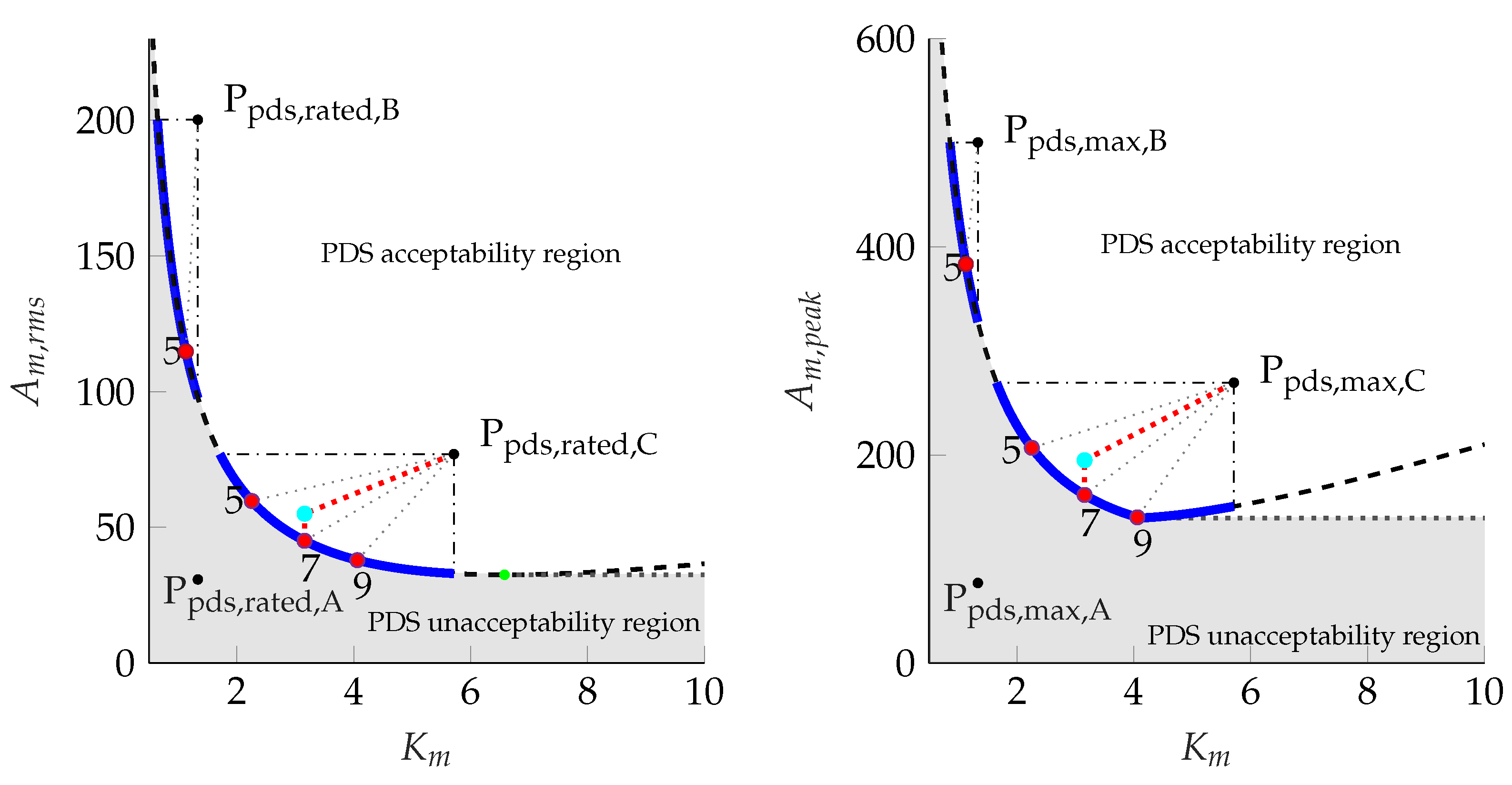
This result is depicted in Figure 2, in which, for clarity, the function A m , r m s ( K m ) together with points P p d s , r a t e d , and A m , p e a k ( K m ) with points P p d s , m a x , have been plotted separately.
In the left panel of Figure 2, the A m , r m s K m function is represented by a dashed black line. A power drive system for which the third quadrant centered at A p d s , r a t e d does not contain an arc of the curve cannot satisfy for any value of K m (or equivalently of i t ) inequality (10); as such, it is rejected as a candidate. This is the case of drive system A.
On the other hand, the third quadrant generated by a P p d s , r a t e d lying outside of the non-acceptability region (which is filled in gray in Figure 2) defines the feasibility arc (highlighted in blue for PDS B and C); the feasibility arc defines a feasibility interval K m , m i n ,   K m , m a x in which an ideal admissible transmission ratio can be found.
An ideal transmission determining, together with the motor inertia, a kinetic factor higher than K p d s , m a x would result in a violation of inequality (8); similarly, a reduction ratio yielding a A m , r m s greater than A p d s , r a t e d would not satisfy inequality (10).
A very similar situation can be seen in the right panel of Figure 2, in which the A m , p e a k K m function is represented in an analogous way along with the points P p d s , m a x characterizing the power drive systems A, B and C. PDS A cannot satisfy inequality (23), while in principle, some ideal transmission can be used to couple the load with drive systems B and C.
Given, however, the discrete nature of the practically available reduction ratios, it remains to be seen whether some of them fall, for a given drive system, within the feasiblity arc. It should be stressed that at this stage, in order to establish a one-to-one correspondence between the reduction ratio i t and the kinetic factor K m , a power drive system (and in particular the motor inertia parameter J m ) has to be chosen.This enables the representation of the discrete points P m , r m s and P m , p e a k corresponding to the available transmission ratios; for an ideal transmission these points will lie on the curves A m , r m s ( K m ) and A m , p e a k ( K m ) . In the figure, it can be seen that, for drive system B, the only available and feasible ideal transmission has a reduction ratio equal to i t = 5 . On the other hand, the power drive system C can be matched with the load through purely kinematic reduction ratios equal to 5, 7 and 9.
At this point, it becomes possible to also consider the effects of the most important transmission non-idealities. These parameters can be taken into account by defining the following quantity:
τ ˜ l = τ l η + i t J t ω ˙ l .
Substitution into Equation (6) yields:
τ m = τ ˜ l ( t ) i t + i t J m ω ˙ l ,
which is formally identical to Equation (7).
The already developed relationships remain, therefore, unchanged. In particular, it can be noted that, on the ( K m A m ) plane, the points associated to the power drive systems will remain unchanged, while the points P m , r m s and P m , p e a k at a given reduction ratio will shift along the vertical direction away from curves A m , r m s ( K m ) and A m , p e a k ( K m ) as an effect of the transmission efficiency and inertia.
Again, these effects can be visualized in order to shed more light on the influence of the main parameters characterizing the non-ideal transmission.
In each panel of Figure 2, in relation to power drive system C, a point P m , r m s and a point P m , p e a k , computed taking into account a non-ideal transmission having reduction ratio equal to 7, have been represented in cyan. Although the introduction of transmission non-idealities results in a fairly typical upward shift of the driven equipment point, it can be seen that such a point remains within the admissibility quadrants originating at P p d s , r a t e d and P p d s , m a x that characterize the drive system. It can be concluded that the servo axis composed by this non-ideal transmission and power drive system C can be properly coupled to the mechanical load. The relationships described above from a graphical point of view can also be further analytically or numerically explored to enable the precise evaluation of the following quantities:
  • The minimum point and the minimum value of A m , p e a k ( K m ) ;
  • The minimum point and the minimum value of A m , r m s ( K m ) ;
  • The feasibility interval K m , m i n ,   K m , m a x for a given drive system.
Given its definition, a fully analytical treatment of the function A m , p e a k ( K m ) is hardly practicable. One useful property of uni-modality (i.e., of the existence and uniqueness of an extremum, in particular of a minimum) can, however, be proven, which in turn guarantees that the numerical processing of this function can make use of classical minimization and root-finding algorithms in a very predictable manner.
An alternative approach to this numerical treatment involves, on the other hand, the definition of a more convenient upper-bound estimate of A m , p e a k K m :
A m , u b e K m = ω l , p e a k K m max t | τ l ( t ) | + K m ω l , p e a k max t | ω ˙ l ( t ) |
= ω l , p e a k K m τ l , p e a k + K m ω l , p e a k ω ˙ l , p e a k A m , p e a k K m .
As also depicted in Figure 3, it can be easily shown that A m , u b e ( K m ) tends to A m , p e a k ( K m ) as either K m approaches zero or infinity. In these regions, both A m , p e a k and A m , u b e asymptotically tend to the same hyperbola or to the same positively sloped straight line. Only in the mid-range, where both curves display a minimum, does A m , u b e appreciably overestimate A m , p e a k . From these properties, it can be concluded that A m , u b e constitutes, for most purposes, an appropriate—while still cautious—approximation of A m , p e a k .
Inequality (9) can then be conservatively replaced with the following:
A p d s , m a x A m , u b e .
The minimum point of A m , u b e can be straightforwardly obtained by requiring that:
d A m , u b e d K m = ω ˙ l , p e a k ω l , p e a k ω l , p e a k τ l , p e a k K m 2 = 0
As a result:
K m , o p t , u b e = ω l , p e a k τ l , p e a k ω ˙ l , p e a k
A power drive system having A p d s , m a x below the minimum value:
A m , u b e ( K m , o p t , u b e ) = 2 τ l , p e a k ω ˙ l , p e a k
cannot satisfy inequality (23), and can be (slightly overcautiously) rejected. Similarly, the minimum point of A m , r m s , which corresponds also to the minimum point of A m , r m s 2 , can be determined by solving the equation:
d A m , r m s 2 d K m = 2 K m ω ˙ l , r m s 2 ω l , p e a k 2 τ l , r m s 2 K m 3 = 0
It can therefore be easily found that:
K m , o p t , r m s = ω l , p e a k τ l , r m s ω ˙ l , r m s
Again, a power drive system characterized by a A p d s , r a t e d below the value:
A m , r m s ( K m , o p t , r m s ) = 2 ( L ¯ l + τ l , r m s ω ˙ l , r m s )
cannot possibly satisfy inequality (10), and is thus eliminated from the pool of candidates. For power drive systems that pass these first tests, it remains to be seen whether they admit a non-null feasibility interval K m , m i n ,   K m , m a x . To do so, it is necessary to rearrange inequalities (23) and (10) to obtain the following:
ω ˙ l , p e a k ω l , p e a k K m 2 A p d s , m a x K m + ω l , p e a k τ l , p e a k 0
K m 4 ω ˙ l , r m s 2 ω l , p e a k 2 + 2 L ¯ l A p d s , r a t e d 2 K m 2 + ω l , p e a k 2 τ l , r m s 2 0
From the solution of the quadratic inequality (30), the feasibility interval K m , m i n , u b e ,   K m , m a x , u b e relative to A m , u b e ( K m ) is obtained.
Similarly, the biquadratic inequality (31) yields the feasibility interval K m , m i n , r m s ,   K m , m a x , r m s relative to A m , r m s ( K m ) .
As a result:
K m , m i n = max ( K m , m i n , u b e , K m , m i n , r m s )
K m , m a x = min ( K m , m a x , u b e , K m , m a x , r m s , K p d s , m a x )
As a final check, it remains to be seen whether
K m , m i n < K m , m a x ,
which is not satisfied for power drive systems having A p d s , r a t e d A m , r m s ( K m , o p t , r m s ) and A p d s , m a x A m , u b e ( K m , o p t , u b e ) but either point P p d s , r a t e d to the left of the graph A m , r m s ( K m ) or point P p d s , m a x to the left of the graph A m , p e a k ( K m ) .

2.2. Sizing Procedure

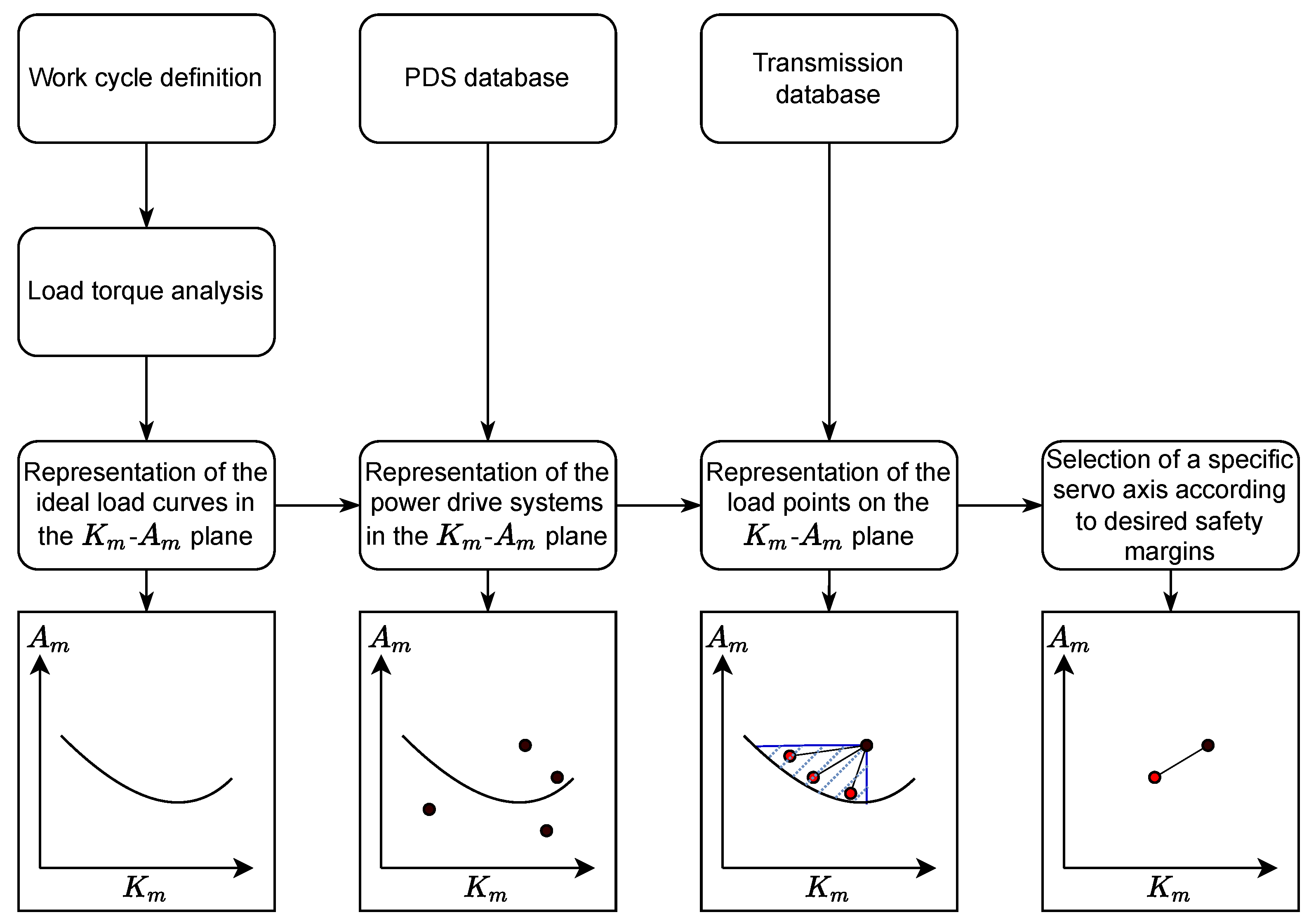
The relationships described above can be integrated into a complete workflow that leads to the sizing of the servo axes of a mechatronic system. Such a workflow, which is summarized in Figure 4, requires firstly the identification of:
  • The load angular velocity at the output shaft ω l ( t ) ;
  • The load angular acceleration at the output shaft ω ˙ l ( t ) ;
  • The load torque at the output shaft τ l ( t ) ;
  • One or more motors expressed as a pair of points ( P p d s , r a t e d , P p d s , m a x ) ;
  • For each motor, a list of practically matchable transmissions.
Concerning the first three points, it should be observed that the definition of the quantities ω l ( t ) , ω ˙ l ( t ) and τ l ( t ) at section ( l ) requires not only a model that can, as a minimum, account for the inverse kinematics and dynamics of the machine, but also the definition of a reference work cycle as representative as possible of the real tasks to be executed by the device. These steps will be exemplified in detail in the following sections.
Regarding the last point, on the other hand, it should be noted that, along with the main transmission parameters of theoretical interest that have been described in the previous section, other practically important properties can help to define a set of transmissions reasonably matchable with each power drive system. These properties concern, primarily, the type of the transmission, its geometrical size, the admissible velocities at the motor shaft and the maximum torques at the output.
In particular, having defined the type in relation to the target application, it is good practice to match the mechanical properties of the transmission not so much to the load, which is always imperfectly modelled, but rather to the power drive system, which, on the contrary, is well-defined in terms of size and of maximum admissible velocities and torques.
This allows a preliminary definition, for each candidate power drive system, of a short list of geometrically and mechanically appropriate transmissions having different reduction ratios, efficiencies and inertias.
These preparatory phases are represented in the topmost blocks of the flowchart reported in Figure 4.
After the full specification of the mechanical load and the definition of a database of power drive systems, it is possible to visualize, as detailed in the preceding section, the main inequalities under the assumption of ideal transmissions. This allows the rejection of the drive systems that cannot, in any case, be matched to the load, and also—more qualitatively—of those that are clearly oversized.
In relation to the points P p d s , r a t e d and P p d s , m a x of each remaining candidate power drive system, it is then possible to highlight the points P m , r m s and P m , p e a k corresponding to the shortlisted transmissions.
The selection of a specific transmission for a given power drive system can then be performed by considering another output of the procedure, which is constituted by the safety factors defined for each feasible servo-axis unit. These safety factors are related to the peak velocity ( M v ), to the rated torque ( M τ , r a t e d ), to the peak torque ( M τ , p e a k ), and to the upper bound estimate of the torque ( M τ , u b e ):
M v = ω p d s , m a x ω m , p e a k
M τ , r a t e d = τ p d s , r a t e d τ m , r m s
M τ , p e a k = τ p d s , m a x τ m , p e a k
M τ , u b e = τ p d s , m a x τ m , u b e
For a given servo axis, these quantities can be easily evaluated to quantify the ratio between the capabilities of the power drive system and the requests of the load projected at the motor shaft.
These safety factors can also be equivalently expressed in terms of K m and A m , and thus can be estimated from the graphical representation exemplified by Figure 2. It can indeed be shown that:
M v = K p d s , m a x K m
M τ , r a t e d = A p d s , r a t e d A m , r m s
M τ , p e a k = A p d s , m a x A m , p e a k
M τ , u b e = A p d s , m a x A m , u b e
The final choice among the feasible PDS and transmission pairs should be made in order to obtain appropriate velocity and torque safety factors.
For a fixed-power drive system, it should be considered that different transmissions will strike a different balance between the velocity and torque safety factors. It is often helpful, then, to take into account the fact that the kinematics of the load are often predicted (or dually enforced) with good accuracy, while the dynamics are often subject to considerable uncertainty owing, e.g., to imperfectly modelled frictional actions or to off-design operating conditions. In addition, it can be easily seen that the non-idealities of the transmission do not affect M v in any way, while, on the other hand, they usually lead to a reduction in the torque-related safety factors. It is therefore often appropriate to select a transmission that can grant good torque safety factors even at the expense of the velocity margin.

3. Case-Study Description

The general procedure described in the previous sections is applicable to any multi-degree of freedom machinery; it is independent to the specific kinematic configuration of the system. The feasibility of the procedure is here demonstrated through a complex test case, i.e., a parallel kinematics robotic system, characterized by a delta-like structure. This system presents the following features:
  • Multiple degrees of freedom;
  • Configuration-dependent and coupled inertial parameters;
  • Mixed loads in which neither the dynamic actions nor the static contributions can be neglected.
As already briefly introduced, the analysis of the mechanical load constitutes the groundwork upon which the servo-axis selection procedure will be constructed. For robotic systems, this entails not only a sufficient knowledge of the manipulator’s kinematics and dynamics, but also the definition of a reference motion cycle which must be representative of the actual working conditions of the device.
The first problem can be obviated by the use of multibody dynamics simulation tools, which allow the quick definition of the accurate virtual models of the target mechanism. On the other hand, if such software is not available, general analytical or numerical techniques must be applied. It must be stressed that, to obtain the motion and torques at the output shaft of the transmission given the movement of the end effector, at least the inverse kinematics and dynamics of the robot must be solved.

3.1. Mechanical Analysis

The parallel kinematic manipulator (PKM) under analysis has already been described in greater detail by the authors in [33]. While the main concern of that work was the study of vibration dynamics around fixed equilibrium positions, here, on the contrary, the compliance of the belt elements forming the linear transmission is neglected. On the other hand, fully non-linear (rather than linearized) dynamics are needed for the purposes of motor sizing and transmission selection. The main results of the mechanical analysis of the robot are therefore summarized in the following discussion.
The device, along with its main characteristic dimensions, is depicted in Figure 5. The notable points and vector loop closures needed for the kinematic analysis are reported in Figure 6.
The main properties of the robot structure are:
  • The three linear axes are parallel to each other.
  • Each linear axis is composed of a linear belt transmission, which is assumed to be stiff; the elements of vector q represent the rotations of the actuated pulleys, which have radius R p ; q ˜ = R p q is introduced to represent the translation of the carts.
  • The motors will be connected to the actuated pulley of the linear belt transmission by means of a planetary transmission.
  • The maximum axis stroke is 1.2 m.
  • The distance l r between two consecutive axes is 200 mm.
  • The length l d of the links connecting the carriages to the end effector is 400 mm.
The kinematics of the manipulator are largely analogous to those of the Delta robot designed by Reymond Clavel [34]; as such, this mechanical structure results in a mobile platform having three translational degrees of freedom.
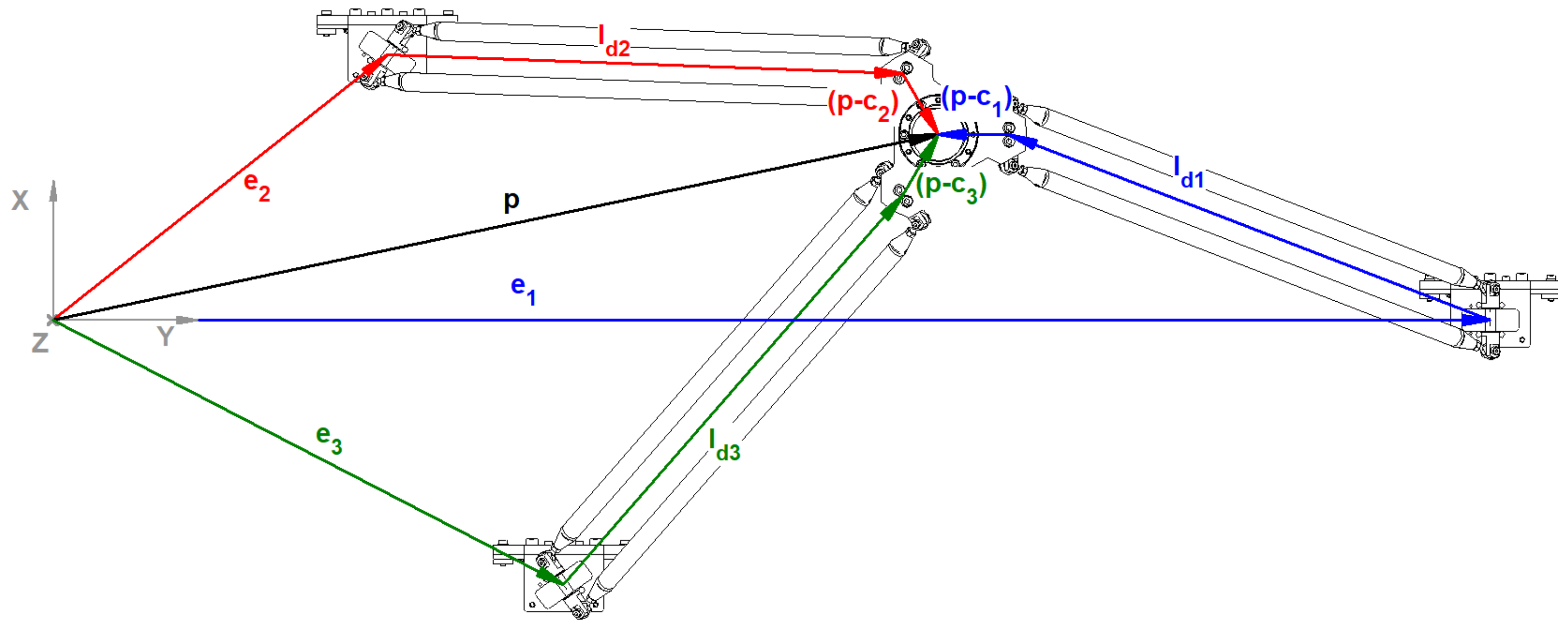
The coordinates q ˜ 1 , q ˜ 2 and q ˜ 3 , which can be used to describe the kinematics of the manipulator, are those relative to the longitudinal displacement of the three trucks. Given the geometric parameter l r that defines the distance between two adjacent linear guides, the truck positions e j are trivially expressed as functions of q ˜ j :
e 1 = q ˜ 1 0 0 , e 2 = q ˜ 2 l r , 0 , e 3 = q ˜ 3 l r , 0 .
The direct and inverse functions between these quantities and the center point p of the moving platform must, furthermore, be determined. The chief relationships that allow to do so are the vector loop equations written for each kinematic chain:
e j + l d , j + ( p c j ) = p j [ 1 , 2 , 3 ] .
In Equation (44), l d , j is the vector pointing from the jth truck to the jth platform constraint c j , while the difference ( p c j ) is a constant vector entirely determined by the geometry of the moving platform.
The vector loop equations, whose geometric meaning is depicted in Figure 6, must be satisfied for every assembled configuration of the robot. To enforce these equations, given either the platform position p or the truck coordinates q ˜ , both analytical or geometrical methods can be used. In this way, the forward and inverse position kinematics relationships can be obtained; at the same time, the positions of the notable points of the structure can also be determined. The Euler angles describing the orientation of the jth distal rod can also be recovered given the points c j and e j .
Again, through geometric or analytical means, it becomes possible to highlight the Jacobian matrices linking the time derivative of the free coordinates q ˜ ˙ to the velocities of the centers of mass and to the angular velocity of each link. In particular, it is necessary to highlight the Jacobian matrices D e , j , D p , D d , j and D ω , j , such that:
p ˙ = D p q ˜ q ˜ ˙
e j ˙ = D e , j q ˜ q ˜ ˙
d j ˙ = D d , j q ˜ q ˜ ˙
ω j = D ω , j q ˜ q ˜ ˙ .
The symbols d j ˙ and ω j appearing in Equations (47) and (48) indicate, respectively, the velocity of the center of mass and the angular velocity of the jth distal link.
Given the trivial relationship between q ˜ and q , it is necessary to express interchangeably each kinematic quantity as a function of the former or of the latter.
Let m p , m t and m d be the mass of the platform, of each truck and of each distal link; moreover, let I d , j be the inertia tensor of the jth distal link. It is then possible to express the kinetic energy of the system as:
T q , q ˙ = 1 2 R p 2 q ˙ D p m p D p + j = 1 3 D e , j m t D e , j + D d , j m d D d , j + D ω , j I d , j D ω , j q ˙ .
Conversely, the gravitational potential energy of the system is related only to the mobile platform and to the center of mass of the distal links, as only these are allowed to move along the vertical direction.
U g = g 0 0 1 m p p + j = 1 3 m d d j .
The dynamics of the system in symbolic form can finally be obtained by Lagrange’s equations:
d d t T q ˙ T q + U g = Q
The term appearing at the right-hand side of Equation (51) accounts for all the actions that cannot be expressed as derivatives of T and U g , including the external torques acting on the actuated pulleys.
Lagrange’s equations can, finally, be rearranged into a more explicit matrix form, as follows:
M ( q ) q ¨ + C ( q , q ˙ ) q ˙ + F q ˙ + U g = τ .
In Equation (52) M is the mass matrix, C is the matrix related to Coriolis and centrifugal terms, and F accounts for viscous friction effects. On the right-hand side of the equation, the vector τ represents the external torques acting on the actuated pulleys. It is clear from this formulation that inertial, centrifugal, Coriolis, viscous and gravitational terms are included in the vector of joint actions, from which the load torque τ l required at section ( l ) for each motion axis are extracted.
For the following numerical analyses, it is assumed that:
  • m t = 1   k g ,
  • m d = 0.7   k g ,
  • m p = 1.5   k g .
Finally, under the hypothesis of a symmetric mass distribution, the distal link inertia was calculated in the principal and barycentric frame as
I ˜ d , j = m d l d 2 12 1 0 0 0 1 0 0 0 0 .

3.2. Work-Cycle Definition

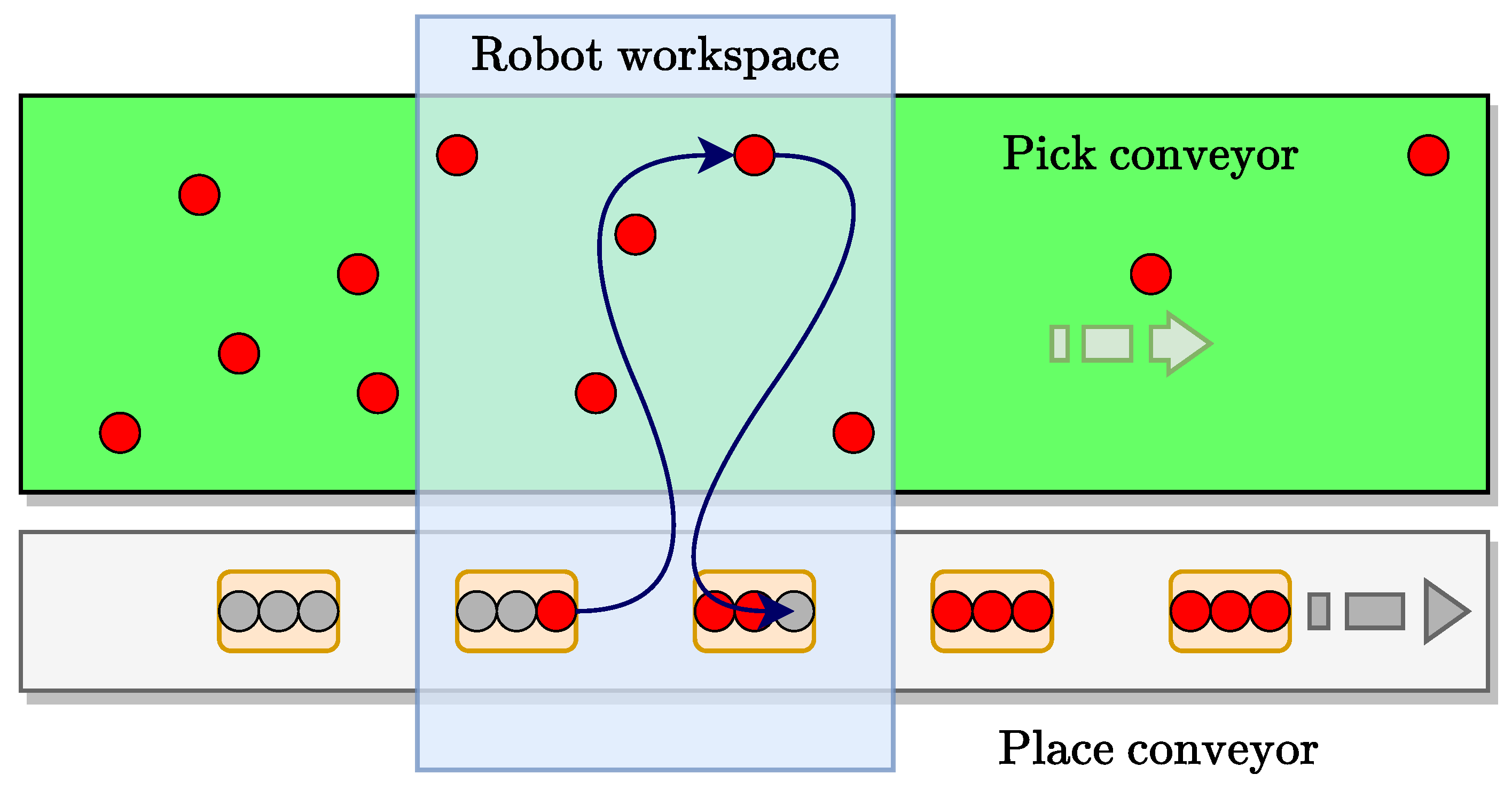
In this work, it is assumed that the robot will be used for pick-and-place operations along two parallel conveyors moving at constant speed. As depicted in Figure 7, the robot has to pick up the moving items carried by one conveyor and deposit them in the boxes carried by the other, in one continuous motion. Each pick-and-place trajectory is constituted by a crossing motion, executed in a horizontal plane at sufficient elevation, and a grasping or deposit motion, executed in the vertical plane along which the moving target is traveling.
Four trajectories broadly covering the robot’s workspace and ultimately forming a closed loop were selected as the reference motion cycle. The working trajectories were designed so as to have a suitable distance from singularities that, as is well-known [35,36], lead to a significant increase in the torques or forces in the robotic system’s legs, and of the joint’s speed. In a general case, the choice of the reference trajectory depends on the kind of multi-degree-of-freedom system, and on the application. The main kinematic characteristics of the hypothesized working cycle are summarized in Table 1.
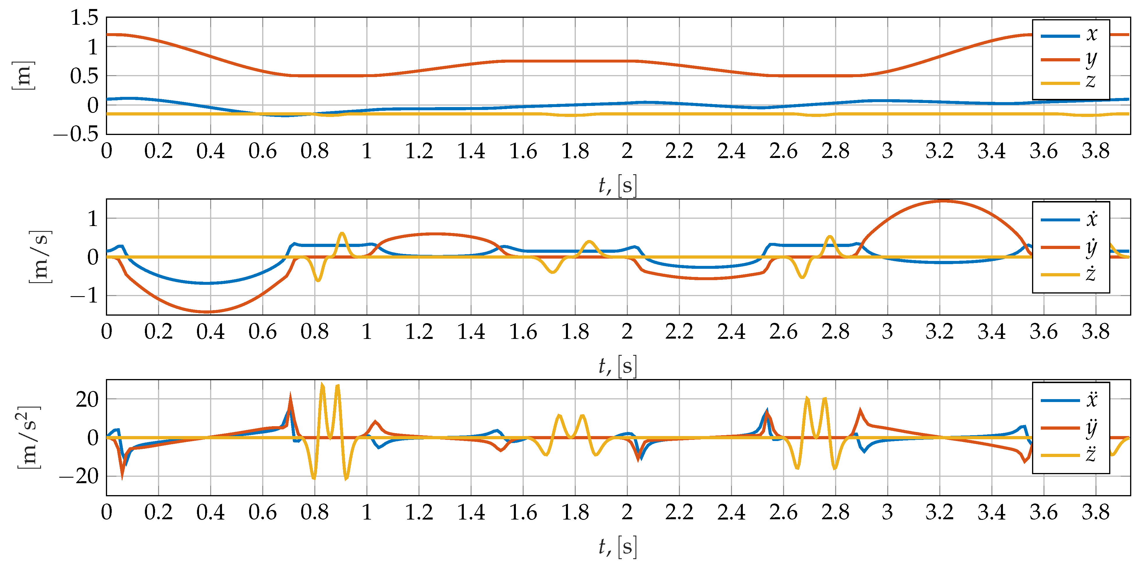
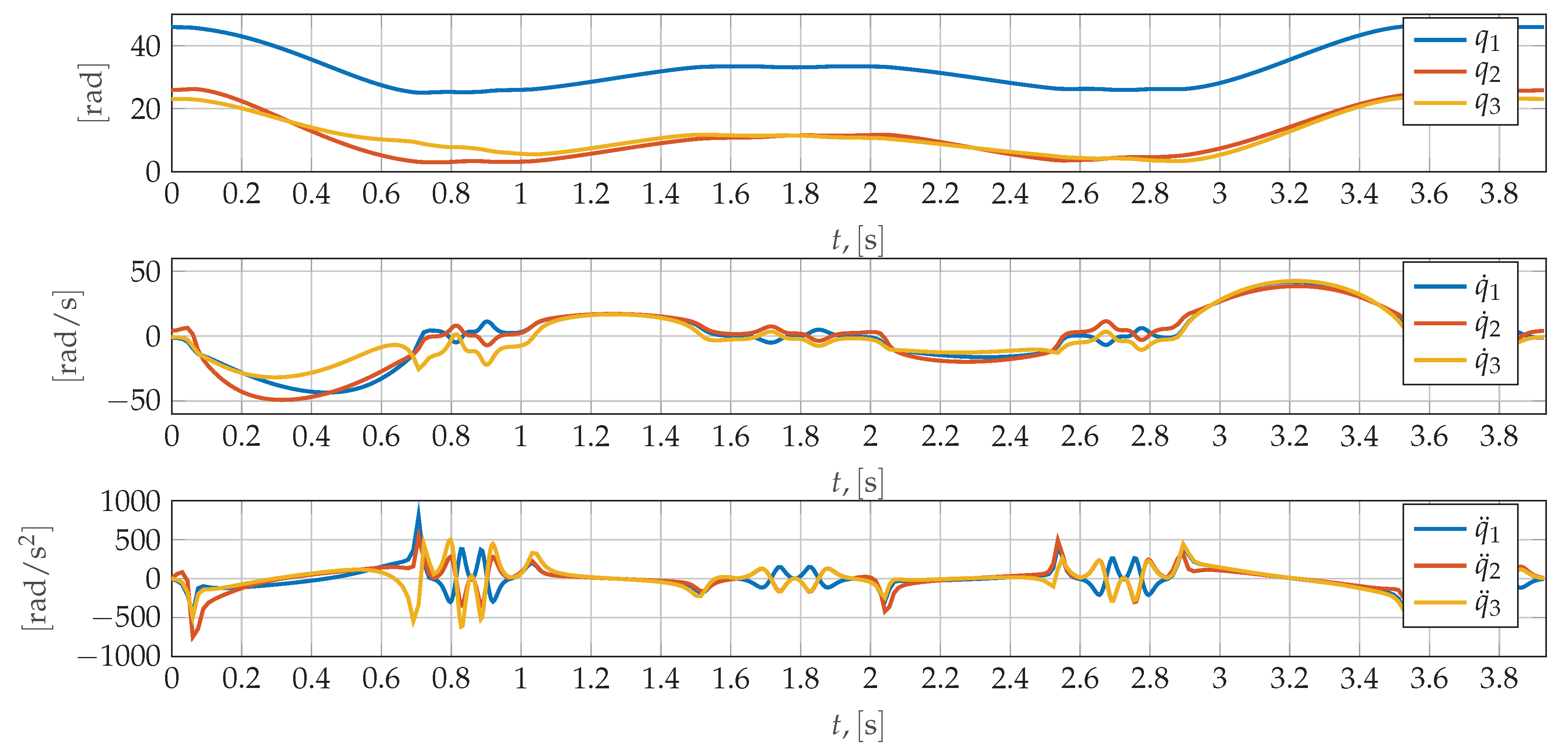
The end-effector trajectories, whose support is represented in Figure 8, were constructed as b-spline curves, whose time parametrization was obtained from velocity boundary conditions selected in order to synchronize the motion of the manipulator with that of the conveyors. The position, velocity and acceleration of the end effector is reported in Figure 9, while the corresponding angular position, velocity and accelerations of the three actuated pulleys are depicted in Figure 10.
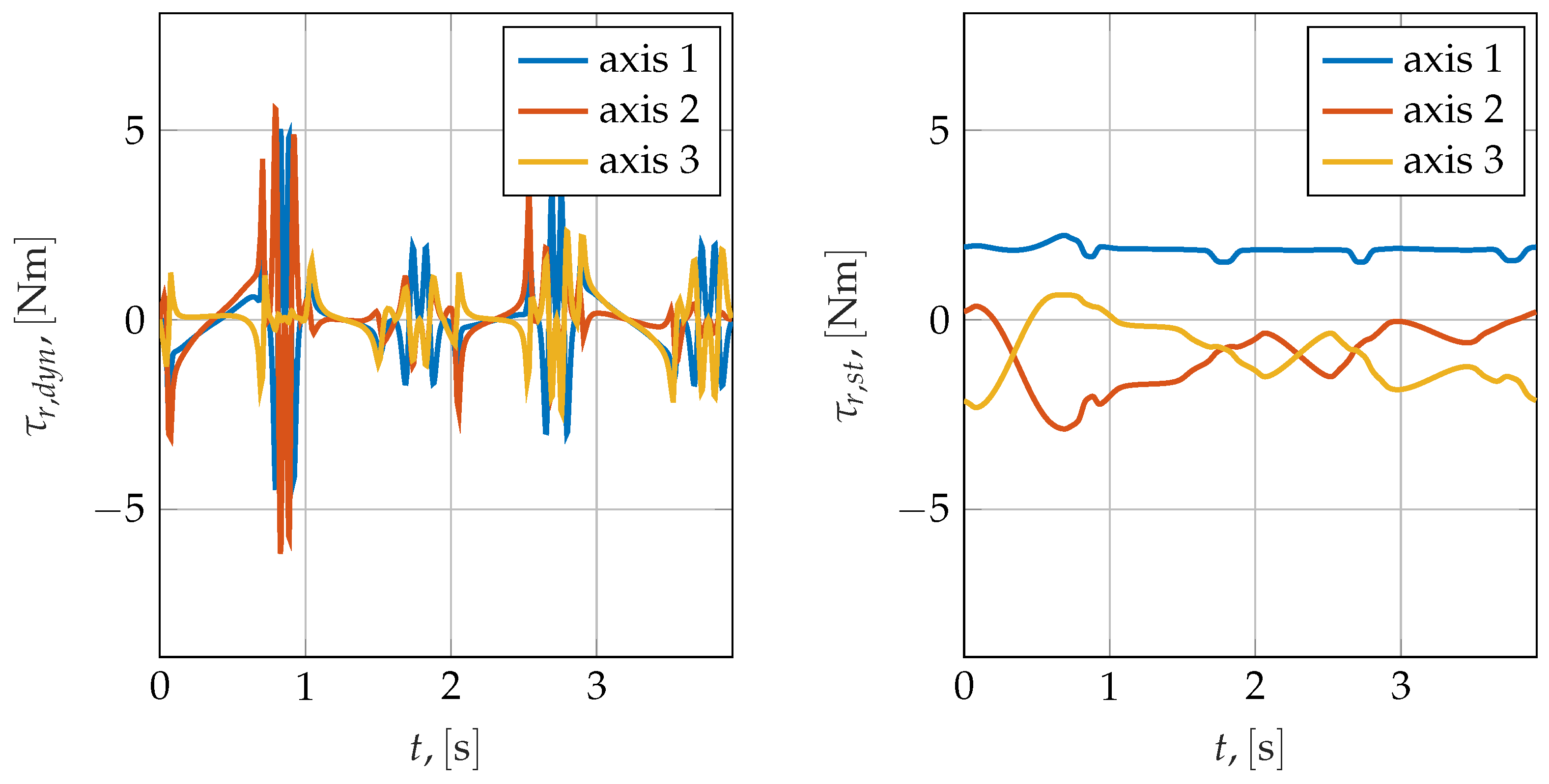
Three different payloads, of 0 kg, 2 kg and 4 kg, were considered to highlight the sensitivity of the required torques to the overall moving masses. The resulting torque profiles, split into dynamic and static contributions, are reported in Figure 11, Figure 12 and Figure 13. As expected, it can be seen that the required static and dynamic torques both increase with the mass of the payload; it should also be remarked how the static contributions, in each considered case, are not negligible with respect to the dynamic ones.

4. Results and Discussion

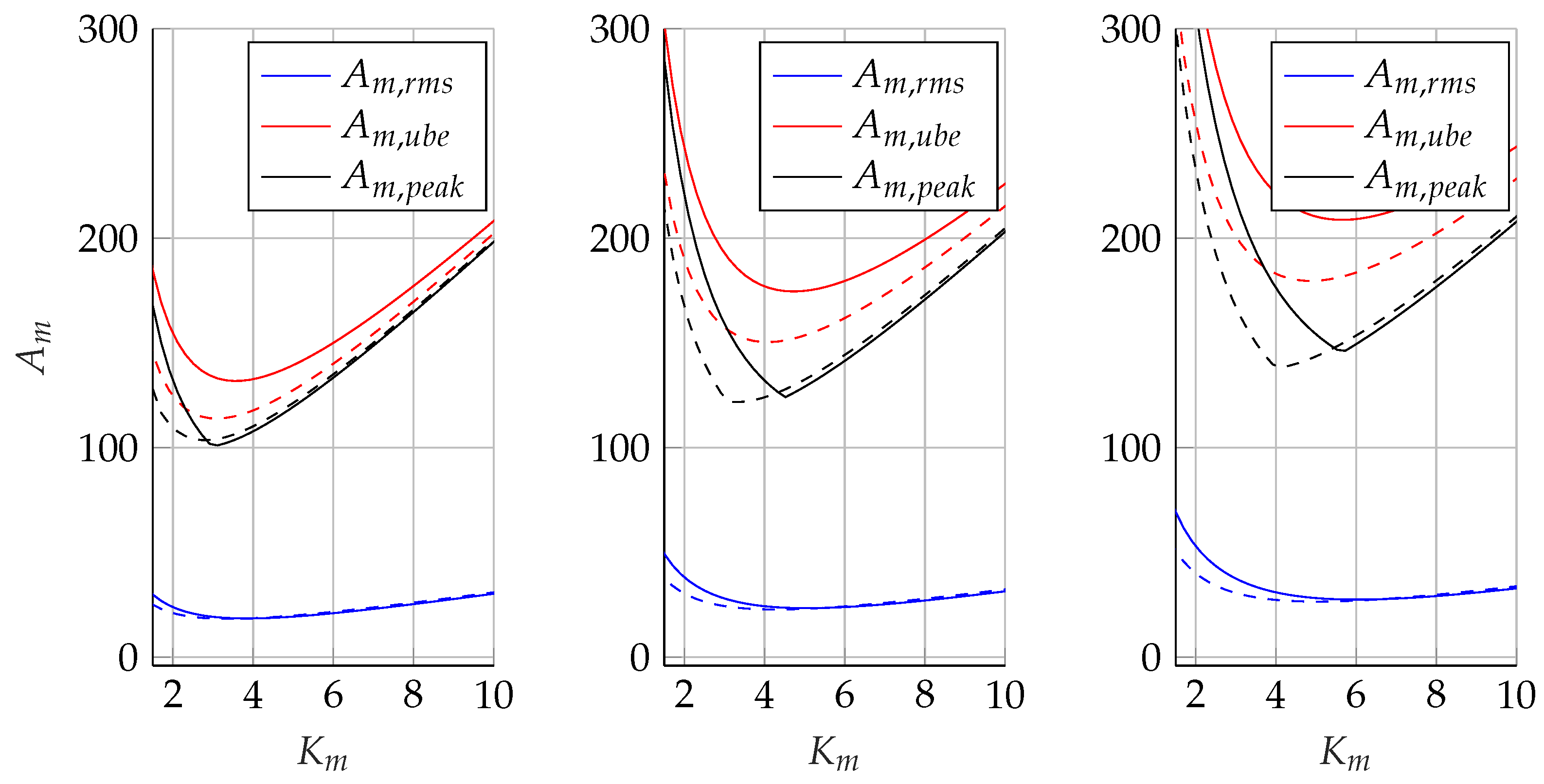
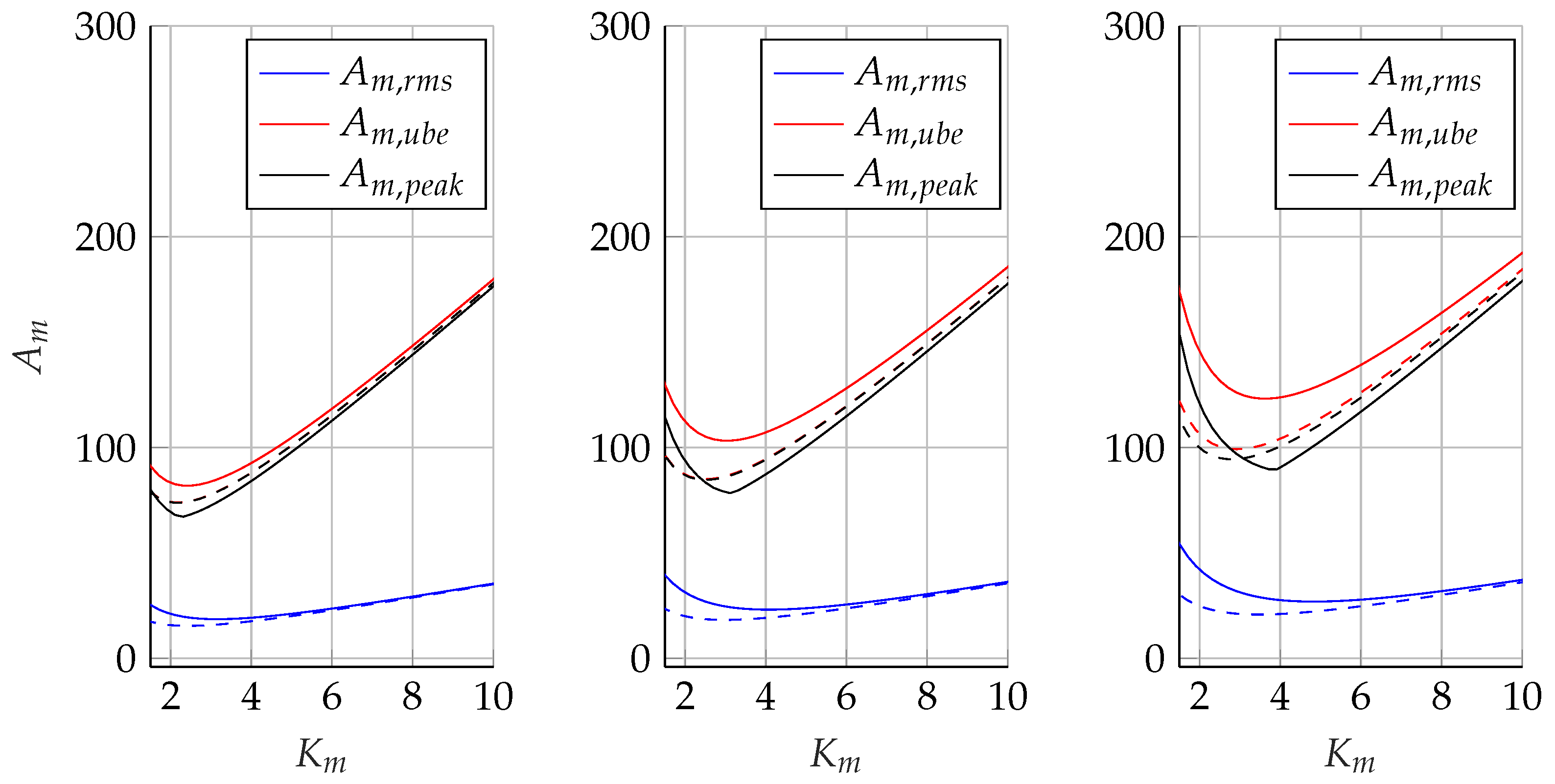
In Figure 14, Figure 15 and Figure 16 the driven equipment curves are plotted in different conditions. In each panel, the dashed lines correspond to purely dynamic loading conditions, while the continuous curves also account for the static loads. Each panel, going left to right, is obtained at different payloads, (0 kg, 2 kg and 4 kg). As expected, it can be seen that both the dynamic and the static contributions increase at increasing payloads; it can also be seen that, for this work cycle, the central axis is characterized by the highest A m , r m s values, which can be attributed to higher static loads. As also suggested by Figure 11, Figure 12 and Figure 13, the highest values for A m , p e a k can be found on axis 2.
In all these diagrams, it can be seen that A m , u b e is a good estimate for A m , p e a k , as K m either increases or decreases towards zero. It can also be observed that, as K m increases, the difference between the driven equipment curves obtained for purely dynamic and for mixed loads decreases. This effect can be easily explained by the fact that K m increases together with the reduction ratio i t ; at higher reduction ratios, in turn, the mechanical load is increasingly dominated by the motor’s own inertia. It is not convenient, however, to size the servo-axis components with the aim of working within this region, which is, at the same time, far from the minima of A m , r m s ( K m ) and A m , p e a k ( K m ) , and characterized by high K m values. As a result, the power drive systems would be grossly oversized, and indeed, it can be qualitatively observed that lighter and smaller power drive systems will tend to be characterized by lower K p d s , m a x , A p d s , r a t e d and A p d s , m a x values.
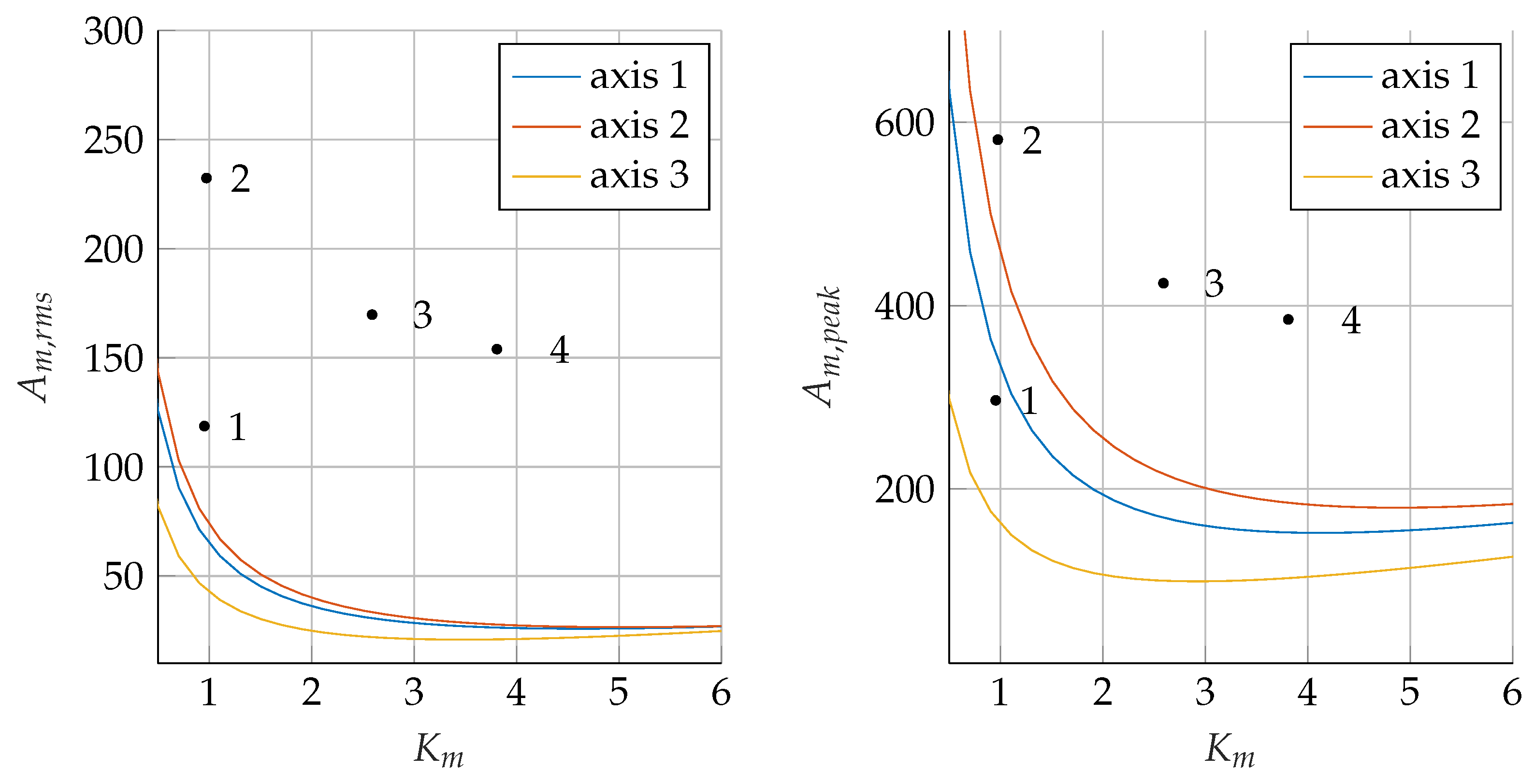
With some caveats, this rule of thumb appears to be broadly confirmed in Figure 17; in the left panel each point represents P p d s , r a t e d for PDS of increasing size, while in the right panel the corresponding P p d s , m a x can be found. According to this subdivision, in the left panel the A m , r m s curve for each motion axis at the highest payload are represented, while on the right panel the corresponding A m , p e a k curves can be found. The properties characterizing the considered PDS candidates are also reported in Table 2; these data have been collected from a catalogue of Mavilor motors matched with the Infranor drivers suggested by the constructor.
By observing Figure 17 it can be seen that power drive systems 1 and 2 cannot be applied to all axes, while either PDS 3 or 4 could be selected and applied to actuate each degree of freedom of the robot. The drive system 5 could be adopted if higher safety margins are desired, while 6, 7 and 8 are likely oversized for the application.
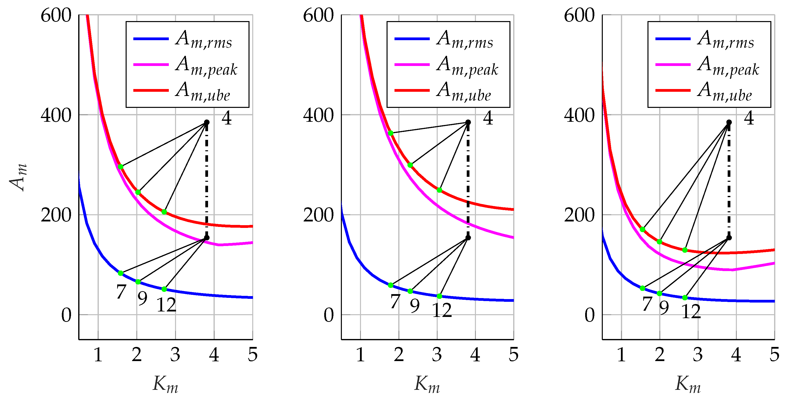
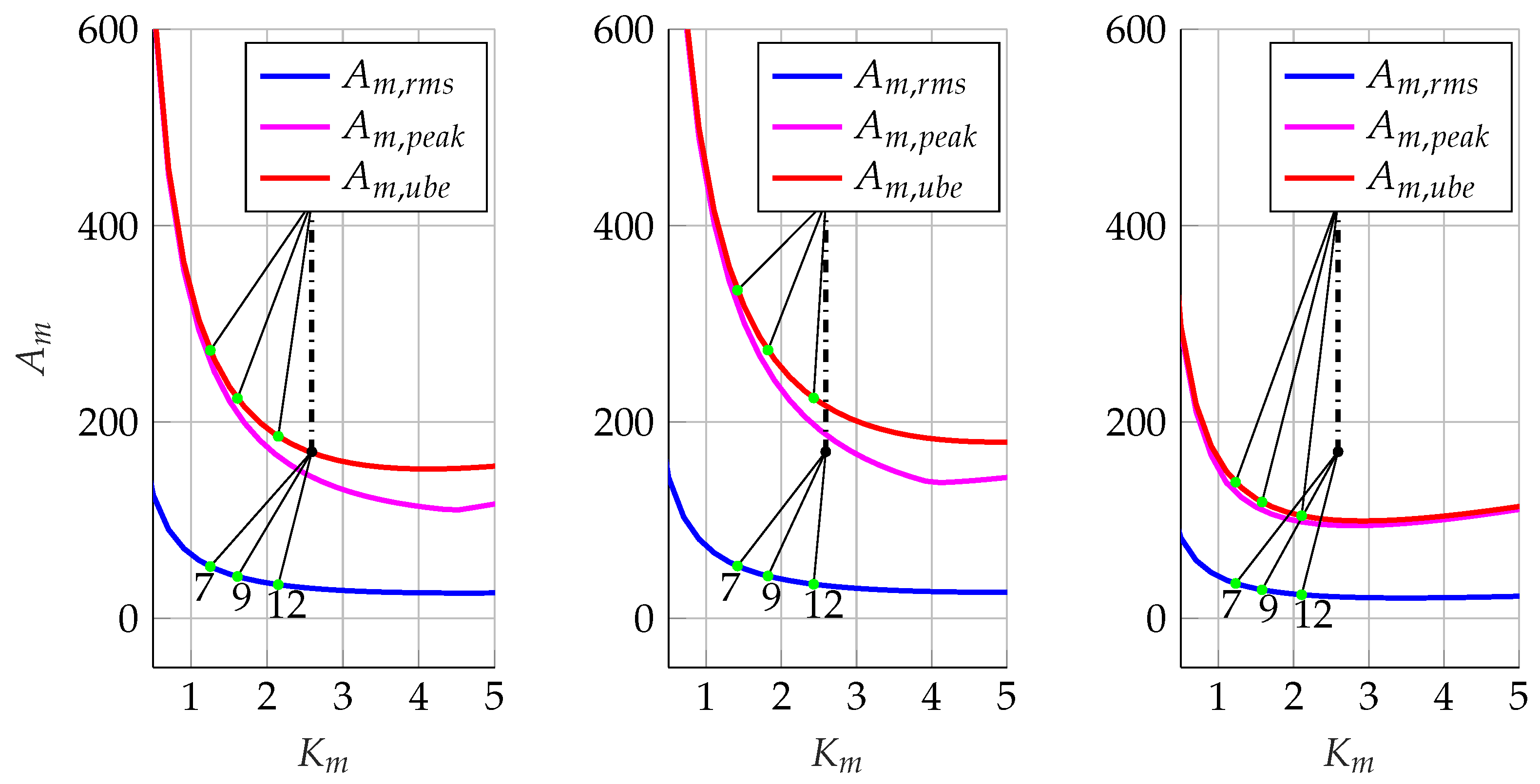
Having oriented the choice toward PDS 3 and 4, it is possible to represent on each load curve the actually available reduction ratios. Figure 18 represents for each axis (axis 1 to 3 from left to right) the two candidate drive systems and their relationship with the driven equipment curves, in term of relative position. The blue curve refers to the root mean square value of the load torque, the magenta one is the peak curve, while the red one corresponds to the upper bound estimate of the peak curve. Moreover, in Figure 18 the load points referred to ideal transmissions that are physically matchable with the motors are presented, along with the corresponding reduction ratio value. For the choice of PDS and transmission, which determines the system’s load point, one of the suitable criteria is the evaluation ot the torque and speed margins that are desirable for the application, depending on whether the major uncertainty is on the loads or on the motion. If we want a similar margin for both torque and speed, we can observe that for both power drive systems a reduction ratio i t = 7 or i t = 9 appear to afford reasonable margins with respect to K m (and ω m ), to A m , r m s (and τ m , r m s ) and to A m , p e a k (and τ m , p e a k ).
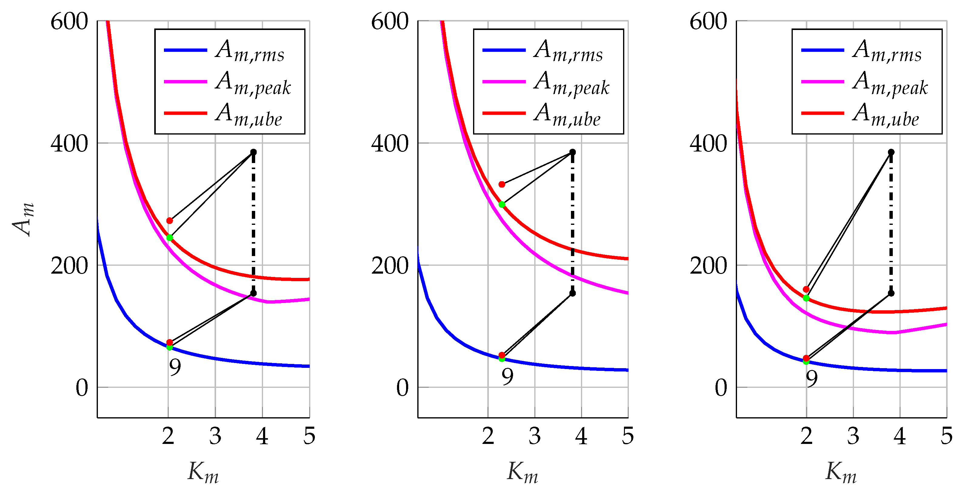
If we want to proceed with an actual transmission ratio rather than an ideal one (which is characterized just by its kinematic parameter i t ), also its moment of inertia J t and efficiency η must be taken into consideration. By considering these two parameters, the driven equipment point moves away from the driven equipment curve, as shown in Figure 19 where, for the PDS 4 the displacement of the points P m , r m s and P m , p e a k corresponding to i t = 9 is highlighted for each axis. For this case, where the values η = 0.9 and J t = 0.07 × 10 4   k g m 2 are assumed, the load points move upwards in vertical direction, according to Equation (19). Both for ideal and actual transmissions, the safety margins obtained for each axis have been evaluated and reported in Table 3.
For the choice of the transmission, once the power drive system has been chosen, other considerations can be made in order to compare the different possible choices that, in this case, are among the three transmissions characterized by i t = 7 , i t = 9 , and i t = 12 . Such another consideration concerns how the motor’s and transmission’s inertia are reflected on the output shaft, and so which is the influence of such inertia on the load. If an ideal transmission is considered, this evaluation can be performed by means of the parameter κ , defined in Section 2.1. As a matter of fact, with κ being the square root of the motor’s inertia reflected to the output shaft, the relevant additional torque can be written as:
τ a m = κ 2 ω ˙ l
If an actual transmission is considered, this evaluation can be performed in a similar way, also including in the parameter κ the motor’s inertia J m , the transmission’s inertia J t , and the transmission’s efficiency η . The new parameter can be defined as:
κ * = i t J m + J t η
and so, the increase in torque on the output shaft can be written as:
τ a m t = κ * 2 ω ˙ l
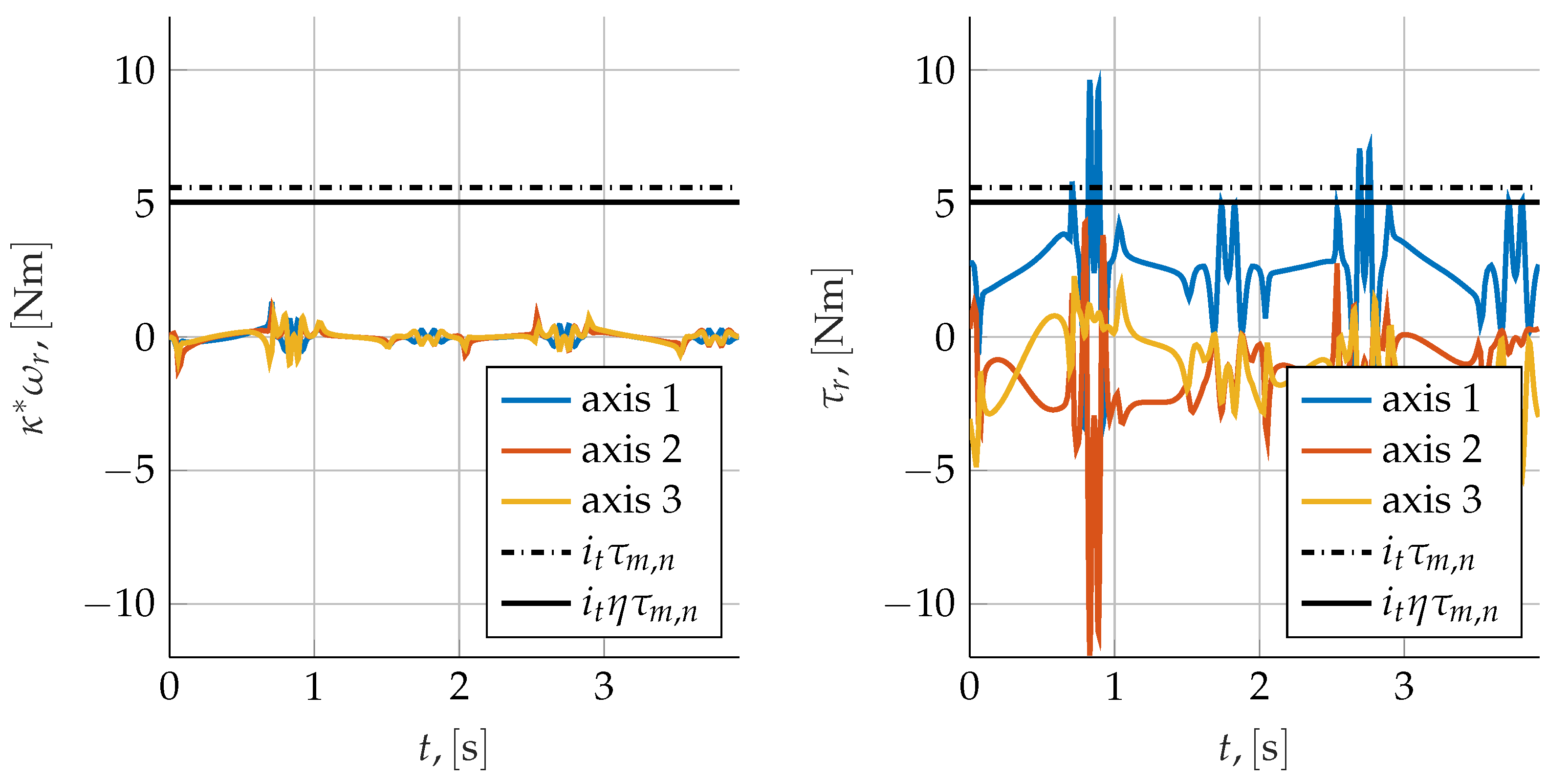
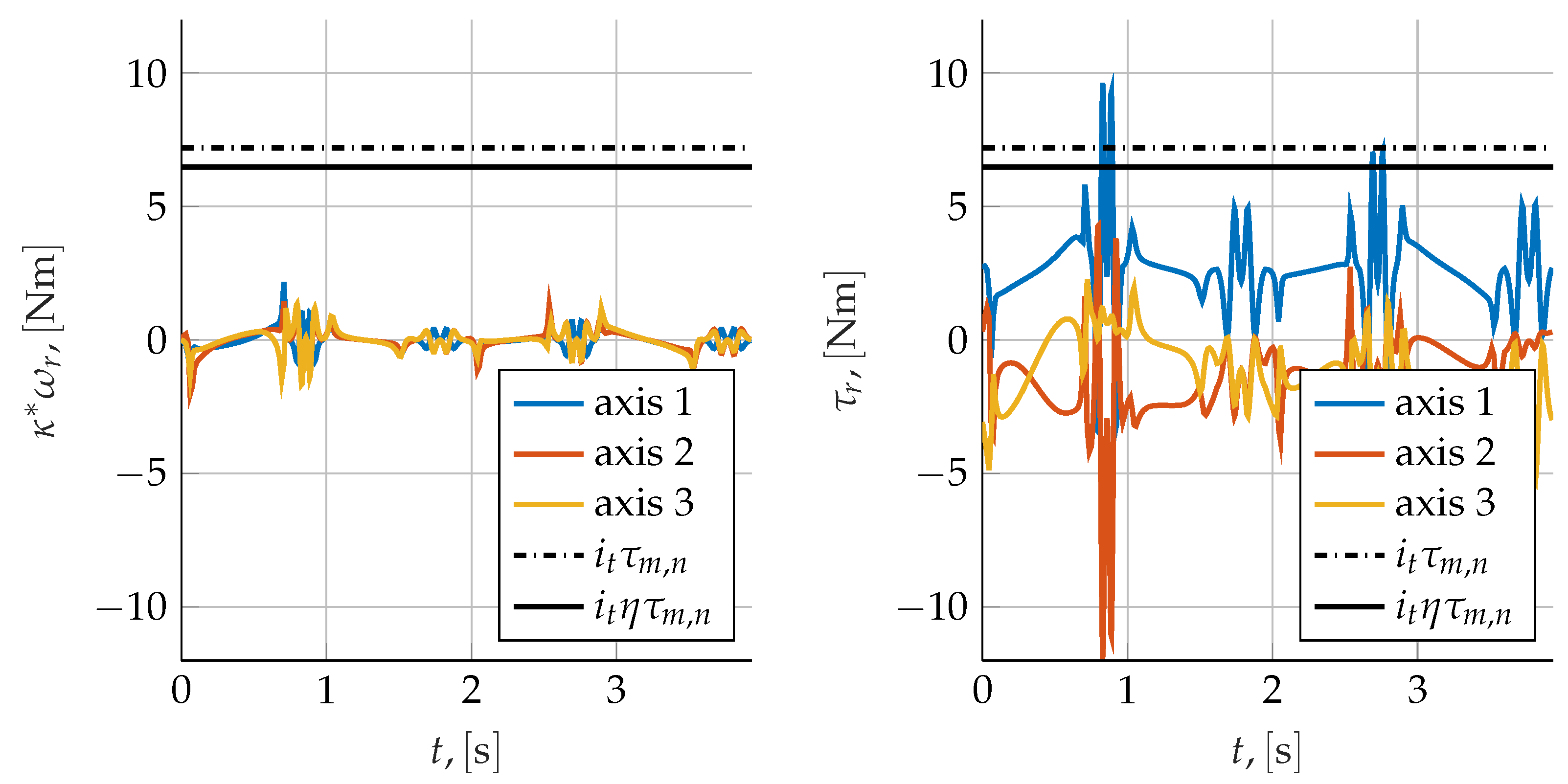
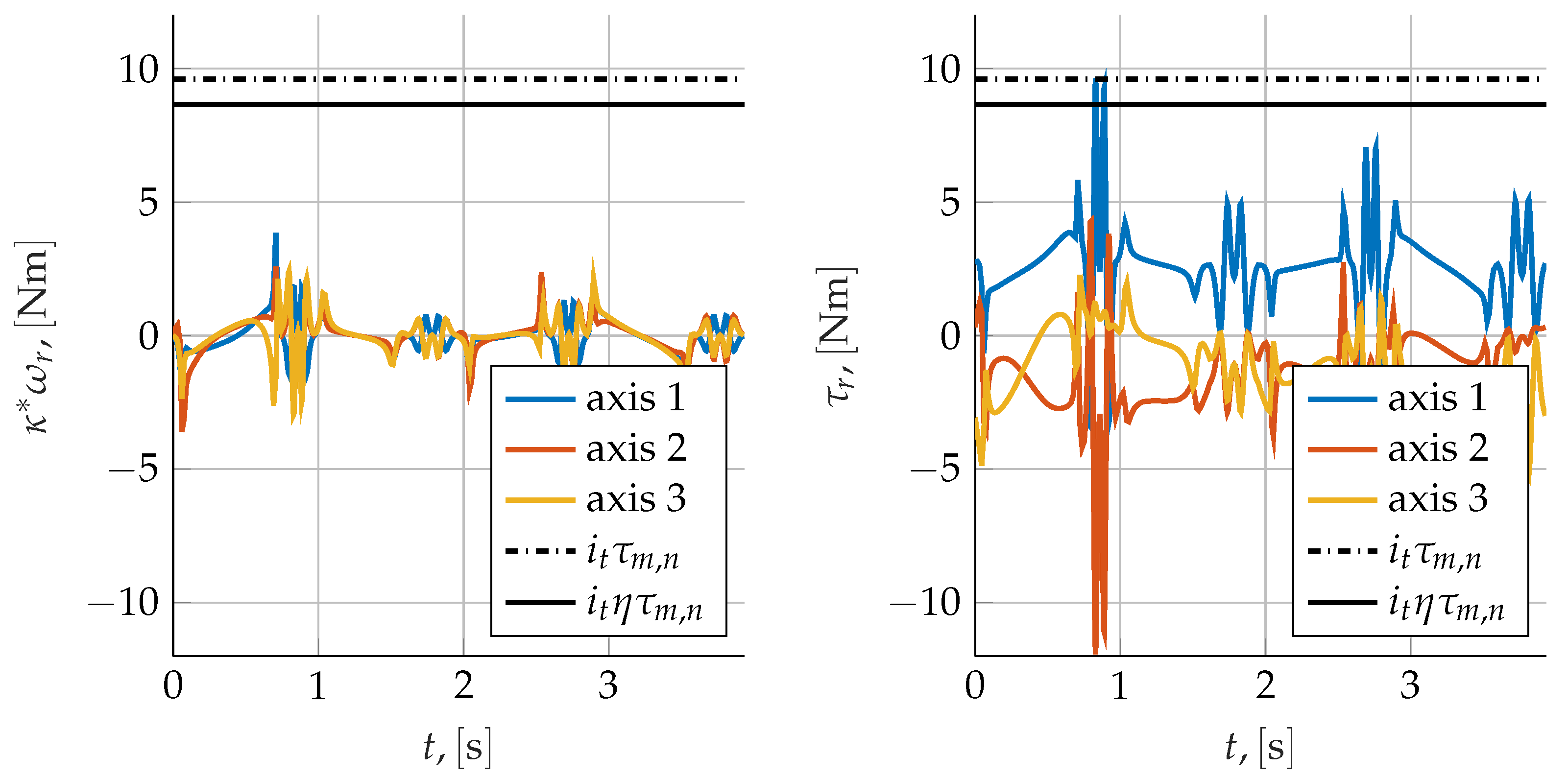
Figure 20, Figure 21 and Figure 22 show, for the three different transmissions, the motor and transmission inertial torques expressed at section ( l ) (left panel), and the load torques (right graph). From the analysis of the graphs, it is clear that the contribution due to the presence of motor and transmission is quite low with respect to the load torque, for all the three cases. However, it is evident that, by increasing the reduction ratio, the contributions increase as well, even if the load torque remains dominant. The graph are completed with two black lines representing the rated torque of the power drive system reduced to the output shaft through an ideal (dashed line) and non-ideal (continuous line) transmission. Obviously, these torques also increase as the reduction ratio increases; moreover, it should be noted that the increment in the reflected maximum and rated torques of the PDS largely compensate for the increase in the motor shaft inertia torques.

4.1. Time Domain Validation

To show the correctness of the proposed approach, the absolute values of the total torques (load torque and torque due to motor and transmission inertia) reflected to the motor’s shaft are reported in Figure 23. On the diagrams are also drawn horizontal straight lines representing the peak and rms values of the load and the nominal and maximum torques of the power drive system. In details, the upper panel shows that the inequality (3) is satisfied, and similarly the bottom panel shows that the peak torques are in the bounds defined by inequality (2). Numerical quantification of the depicted results also confirm the exactness of the entity of the expected velocity and torque safety margins, thus confirming that the results expressed in the ( K m A m ) plane match those obtained from an analysis in the time domain.

4.2. Purely Inertial Loading Conditions

Within this work, much emphasis has been placed on the fact that the proposed method can straightforwardly deal with the selection problem of servo axes for machines working under mixed load; it should be remarked, however, that the same procedure is also applicable without any modification to purely inertial loading conditions. To highlight this, a separate test case was obtained from the application previously described by simply neglecting any non-dynamic action appearing in Equation (52). The results of the analysis of this ancillary test case are reported in Figure 24, Figure 25 and Figure 26. The most likely PDS candidates appear to be 2 and 3 (Figure 25); the analysis of the actually available reduction ratios suggests that PDS 3 is a safer choice, as then confirmed in Figure 26.

5. Conclusions

This paper presents a general procedure for the direct design of the servo axes of multi-degree-of-freedom machinery subject to mixed loads and dynamic coupling due to the mechanical configuration. The definition of the procedure is supported by a theoretical approach, where speed and torque limits are widely and thoroughly discussed and developed. Such theoretical discussion allows to obtain a comprehensive knowledge of the problems related to the simultaneous choice of the PDS and the transmission for each servo axis. The procedure allows to overcome some limitations found in the literature; in particular, the procedure is based only on the knowledge of the torques required at the joints axis and does not need the definition of any constant equivalent inertia of the system projected on each joint axis. The torques include all the loads acting on the system regardless of whether they are related to inertia actions, weight forces, or general external actions. Moreover, the procedure is easily applicable and efficient; In a few steps, it provides a direct choice of the servo-axis components without the need for subsequent iterations, checks or final verification. The procedure proposes a single, concise and comprehensive graphical representation that gives a complete overview of the load, the possible PDSs, and the relevant possible matchable transmissions. To demonstrate the effectiveness of the proposed procedure, it was applied to a linear delta robot characterized by a mixed type load, i.e., both dynamic actions and static actions are present. To show that the procedure is also effective for purely inertial loads, a case widely discussed in the literature, it was applied on the same robot without considering the contribution of the weight forces. The proposed examples prove that the method can efficiently help the designer of a multi-degrees-of-freedom machinery choose the PDS/transmission units and have a deep comprehension of the effect of the different possible choices on the torque ad speed margins of the system’s servo axes.

Author Contributions

Conceptualization, P.R.; methodology, P.R.; software, F.C.; validation, P.R. and R.S.; investigation, P.R., R.S. and F.C.; writing—original draft preparation, P.R., R.S. and F.C.; supervision, P.R. All authors have read and agreed to the published version of the manuscript.

Funding

The APC was funded by the University of Bergamo.

Institutional Review Board Statement

Not applicable.

Informed Consent Statement

Not applicable.

Data Availability Statement

Not applicable.

Conflicts of Interest

The authors declare no conflict of interest.

Nomenclature

Quantities related to the sizing procedure
A m Accelerating factor at the motor shaft.
A m , p e a k Peak accelerating factor actually reached at the input shaft of the transmission.
A m , r m s RMS accelerating factor reached at the input shaft of the transmission.
A m , u b e Upper bound estimate of the peak accelerating factor reached at the input shaft of the transmission.
A p d s , m a x Maximum admissible accelerating factor characterizing the power drive system.
A p d s , r a t e d Rated accelerating factor of the power drive system.
η Efficiency of the transmission.
i t Reduction ratio of the transmission.
J m Inertia of the motor.
J t Inertia of the transmission expressed at the input shaft.
K m Kinetic factor at the motor shaft.
K m , m a x Maximum admissible K m for a given PDS—load pair
K m , m i n Minimum admissible K m for a given PDS—load pair
K m , o p t , r m s Optimum kinetic factor minimizing the A m , r m s function.
K m , o p t , u b e Optimum kinetic factor minimizing the A m , u b e function.
K p d s , m a x Maximum admissible kinetic factor characterizing the power drive system.
L ¯ l Integral average of the product ω ˙ l ( t ) τ l ( t ) .
M τ , p e a k Peak torque safety margin.
M τ , r a t e d Rated torque safety margin.
M τ , u b e Safety margin related to the peak torque upper bound estimate.
M v Peak velocity safety margin.
P m , p e a k Point in the ( K A m , p e a k ) plane characterizing the actual working conditions.
P m , r m s Point in the ( K A m , r m s ) plane characterizing the actual working conditions.
P p d s , m a x Maximum admissible point in the ( K m A m ) plane characterizing the power drive system.
P p d s , r a t e d Rated point in the ( K m A m ) plane characterizing the power drive system.
q Array collecting the positional coordinates of the mechanism’s actuated joints.
τ l Torque at the output shaft of the transmission.
τ l , p e a k Peak torque actually reached at the output shaft of the transmission.
τ l , r m s RMS torque at the output shaft of the transmission.
τ m Torque at the input shaft of the transmission.
τ m , p e a k Peak torque actually reached at the input shaft of the transmission.
τ m , r m s RMS torque at the input shaft of the transmission.
τ m , u b e Upper bound estimate of the torque required at the motor shaft.
τ p d s , m a x Maximum admissible torque characterizing the power drive system.
τ p d s , r a t e d Rated torque characterizing the power drive system.
T c Execution time of the work cycle.
τ ˜ l Augmented load torque at the output shaft of the transmission.
ω l Angular velocity at the output shaft of the transmission.
ω ˙ l Angular acceleration at the output shaft of the transmission.
ω ˙ l , r m s RMS angular acceleration at the output shaft of the transmission.
ω l , p e a k Peak angular velocity actually reached at the output shaft of the transmission.
ω ˙ l , p e a k Peak angular acceleration actually reached at the output shaft of the transmission.
ω m Angular velocity at the input shaft of the transmission.
ω ˙ m Acceleration at the input shaft of the transmission.
ω m , p e a k Peak angular velocity reached at the input shaft of the transmission.
ω p d s , m a x Maximum admissible angular velocity characterizing the power drive system.
General Dynamic quantities
C Matrix of the Coriolis and centrifugal terms.
F Matrix of the viscous friction coefficients.
gGravitational constant.
M Mass matrix of the mechanical system.
Q Array of the external generalized actions.
τ Generalized external actions on the actuated joints.
U g Gravitational potential energy.
V g Gravitational potential.
Quantities related to the applicative example
c j Position of the constraint acting between the jthdistal linkage and the end-effector.
d j Center of mass of the jthdistal link.
D d , j Jacobian matrix associated to d I j .
D e , j Jacobian matrix associated to the jthtruck.
D p Jacobian matrix associated to p .
D ω , j Jacobian matrix associated to ω I j .
e j Position of the jthtruck.
I d , j Inertia tensor of the jthdistal link.
I ˜ d , j Inertia tensor of the jthdistal link expressed in the principal barycentric frame.
l d Length of the distal link.
l d , j Vector pointing from the jthtruck to the jthplatform constraint.
l r Distance between two consecutive linear guides of the linear delta robot.
m d Mass of each distal link.
m p Mass of the moving end-effector platform.
m t Mass of each truck.
p Position of the end-effector platform.
q ˜ j Coordinate describing the longitudinal position of the jthtruck.
q ˜ Array of the coordinates describing the longitudinal position of the three trucks.
q ˜ ˙ Array of the coordinates describing the longitudinal velocity of the three trucks.
q ˜ ¨ Array of the coordinates describing the longitudinal acceleration of the three trucks.
R p Radius of the actuated and free pulleys.
TKinetic energy of the mechanism.
ω j Angular velocity of the jthdistal link.

References

  1. IEC 61800: 2021; Adjustable Speed Electrical Power Drive Systems. IEC: London, UK, 2021.
  2. Van De Straete, H.; Degezelle, P.; De Schutter, J.; Belmans, R. Servo motor selection criterion for mechatronic applications. IEEE/ASME Trans. Mechatron. 1998, 3, 43–50. [Google Scholar] [CrossRef]
  3. Van De Straete, H.; De Schutter, J.; Belmans, R. An efficient procedure for checking performance limits in servo drive selection and optimization. IEEE/ASME Trans. Mechatron. 1999, 4, 378–386. [Google Scholar] [CrossRef]
  4. Pasch, K.; Seering, W. On the drive systems for high—Performance machines. J. Mech. Des. Trans. ASME 1984, 106, 102–108. [Google Scholar] [CrossRef]
  5. Cusimano, G. A procedure for a suitable selection of laws of motion and electric drive systems under inertial loads. Mech. Mach. Theory 2003, 38, 519–533. [Google Scholar] [CrossRef]
  6. Cusimano, G. Generalization of a method for the selection of drive systems and transmissions under dynamic loads. Mech. Mach. Theory 2005, 40, 530–558. [Google Scholar] [CrossRef]
  7. Cusimano, G. Optimization of the choice of the system electric drive-device-transmission for mechatronic applications. Mech. Mach. Theory 2007, 42, 48–65. [Google Scholar] [CrossRef]
  8. Roos, F.; Johansson, H.; Wikander, J. Optimal selection of motor and gearhead in mechatronic applications. Mechatronics 2006, 16, 63–72. [Google Scholar] [CrossRef]
  9. Giberti, H.; Cinquemani, S.; Legnani, G. Effects of transmission mechanical characteristics on the choice of a motor-reducer. Mechatronics 2010, 20, 604–610. [Google Scholar] [CrossRef]
  10. Giberti, H.; Cinquemani, S.; Legnani, G. A practical approach to the selection of the motor-reducer unit in electric drive systems. Mech. Based Des. Struct. Mach. 2011, 39, 303–319. [Google Scholar] [CrossRef]
  11. Cusimano, G. Influence of the reducer efficiencies on the choice of motor and transmission: Torque peak of the motor. Mech. Mach. Theory 2013, 67, 122–151. [Google Scholar] [CrossRef]
  12. Cusimano, G. Choice of electrical motor and transmission in mechatronic applications: The torque peak. Mech. Mach. Theory 2011, 46, 1207–1235. [Google Scholar] [CrossRef]
  13. Cusimano, G. Choice of motor and transmission in mechatronic applications: Non-rectangular dynamic range of the drive system. Mech. Mach. Theory 2015, 85, 35–52. [Google Scholar] [CrossRef]
  14. Cusimano, G.; Casolo, F. An almost comprehensive approach for the choice of motor and transmission in mechatronics applications: Motor thermal problem. Mechatronics 2016, 40, 96–105. [Google Scholar] [CrossRef]
  15. Cusimano, G.; Casolo, F. An almost comprehensive approach for the choice of motor and transmission in mechatronic applications: Torque peak of the motor. Machines 2021, 9, 159. [Google Scholar] [CrossRef]
  16. Cusimano, G. Non-rectangular dynamic range of the drive system: A new approach for the choice of motor and transmission. Machines 2019, 7, 54. [Google Scholar] [CrossRef] [Green Version]
  17. Bartlett, H.; Lawson, B.; Goldfarb, M. Optimal transmission ratio selection for electric motor driven actuators with known output torque and motion trajectories. J. Dyn. Syst. Meas. Control Trans. ASME 2017, 139, 101013. [Google Scholar] [CrossRef]
  18. Meoni, F.; Carricato, M. Optimal selection of the motor-reducer unit in servo-controlled machinery: A continuous approach. Mechatronics 2018, 56, 132–145. [Google Scholar] [CrossRef]
  19. Aftab, Z.; Shafi, F.; Shad, R.; Inzimam-Ul-Haq, R.; Saeed, K. Systematic method for selection of motor-reducer units to power a lower-body robotic exoskeleton. J. Appl. Sci. Eng. (Taiwan) 2021, 24, 457–465. [Google Scholar] [CrossRef]
  20. Campolo, D. Motor selection via impedance-matching for driving nonlinearly damped, resonant loads. Mechatronics 2010, 20, 566–573. [Google Scholar] [CrossRef]
  21. Giberti, H.; Cinquemani, S.; Ambrosetti, S. 5R 2dof parallel kinematic manipulator—A multidisciplinary test case in mechatronics. Mechatronics 2013, 23, 949–959. [Google Scholar] [CrossRef]
  22. Han, G.; Xie, F.; Liu, X.J. Optimal selection of servo motor and reduction ratio for high-speed parallel robots. In Lecture Notes in Computer Science (Including Subseries Lecture Notes in Artificial Intelligence and Lecture Notes in Bioinformatics); Springer: Cham, Switzerland, 2015; Volume 9245, pp. 109–120. [Google Scholar] [CrossRef]
  23. Ge, L.; Chen, J.; Li, R.; Liang, P. Optimization design of drive system for industrial robots based on dynamic performance. Ind. Robot. 2017, 44, 765–775. [Google Scholar] [CrossRef]
  24. Padilla-Garcia, E.; Cruz-Villar, C.; Rodriguez-Angeles, A.; Moreno-Armendáriz, M. Concurrent optimization on the powertrain of robot manipulators for optimal motor selection and control in a point-to-point trajectory planning. Adv. Mech. Eng. 2017, 9, 1687814017747368. [Google Scholar] [CrossRef] [Green Version]
  25. Xie, Z.; Xie, F.; Liu, X.J.; Wang, J.; Shen, X. Parameter optimization for the driving system of a 5 degrees-of-freedom parallel machining robot with planar kinematic chains. J. Mech. Robot. 2019, 11, 041003. [Google Scholar] [CrossRef]
  26. Barjuei, E.; Ardakani, M.; Caldwell, D.; Sanguineti, M.; Ortiz, J. Optimal Selection of Motors and Transmissions in Back-Support Exoskeleton Applications. IEEE Trans. Med. Robot. Bion. 2020, 2, 320–330. [Google Scholar] [CrossRef]
  27. Huang, T.; Mei, J.; Li, Z.; Zhao, X.; Chetwynd, D. A method for estimating servomotor parameters of a parallel robot for rapid pick-and-place operations. J. Mech. Des. Trans. ASME 2005, 127, 596–601. [Google Scholar] [CrossRef]
  28. Shao, Z.; Tang, X.; Chen, X.; Wang, L. Inertia match of a 3-RRR reconfigurable planar parallel manipulator. Chin. J. Mech. Eng. (Engl. Ed.) 2009, 22, 791–799. [Google Scholar] [CrossRef]
  29. Liu, Z.; Tang, X.; Shao, Z.; Wang, L. Dimensional optimization of the Stewart platform based on inertia decoupling characteristic. Robotica 2016, 34, 1151–1167. [Google Scholar] [CrossRef]
  30. Kong, Y.; Cheng, G.; Guo, F.; Gu, W.; Zhang, L. Inertia matching analysis of a 5-DOF hybrid optical machining manipulator. J. Mech. Sci. Technol. 2019, 33, 4991–5002. [Google Scholar] [CrossRef]
  31. Righettini, P.; Strada, R.; Remuzzi, A. A mechatronic apparatus for shear stress application on endothelial cells: Design, development and experimental tests. In Proceedings of the 2021 IEEE International Conference on Mechatronics, Kashiwa, Japan, 7–9 March 2021. [Google Scholar] [CrossRef]
  32. Righettini, P.; Strada, R.; Zappa, B.; Lorenzi, V. Experimental set-up for the investigation of transmissions effects on the dynamic performances of a linear PKM. Mech. Mach. Sci. 2019, 73, 2511–2520. [Google Scholar] [CrossRef]
  33. Righettini, P.; Strada, R.; Cortinovis, F. Modal kinematic analysis of a parallel kinematic robot with low-stiffness transmissions. Robotics 2021, 10, 132. [Google Scholar] [CrossRef]
  34. Clavel, R. Delta, a fast robot with parallel geometry. In Proceedings of the 1988 IEEE International Symposium on Industrial Robot, Philadelphia, PA, USA, 28–29 April 1988. [Google Scholar]
  35. Voglewede, P.; Ebert-Uphoff, I. Overarching framework for measuring closeness to singularities of parallel manipulators. IEEE Trans. Robot. 2005, 21, 1037–1045. [Google Scholar] [CrossRef]
  36. Laryushkin, P.; Glazunov, V.; Erastova, K. On the Maximization of Joint Velocities and Generalized Reactions in the Workspace and Singularity Analysis of Parallel Mechanisms. Robotica 2019, 37, 675–690. [Google Scholar] [CrossRef]
Figure 1. Schematic overview of a multi-axis mechatronic system and of its conceptual subdivisions.
Machines 10 00454 g001
Figure 2. Graphical representation of the main sizing relationships. The black points represent the power drive systems; the red points on the blue feasibility arcs represent ideal P m , r m s and P m , p e a k points at different reduction ratios (whose values are also reported). The points in cyan represent P m , r m s and P m , p e a k obtained from one non-ideal transmission in conjunction with PDS C. The unfeasibility region is filled in gray.
Machines 10 00454 g002
Figure 3. Graphical representation of the ratio A m , p e a k ( K m ) A m , u b e ( K m ) , which highlights the relative asymptotic behaviour of A m , p e a k ( K m ) and A m , u b e ( K m ) .
Machines 10 00454 g003
Figure 4. Selection flowchart for the servo axis.
Machines 10 00454 g004
Figure 5. Diagram of the linear delta.
Machines 10 00454 g005
Figure 6. Vector loops for the three kinematic chains.
Machines 10 00454 g006
Figure 7. Pick-and-place reference task.
Machines 10 00454 g007
Figure 8. Support of the end-effector trajectory hypothesized as a reference cycle.
Machines 10 00454 g008
Figure 9. Position, velocity and acceleration components at the end effector.
Machines 10 00454 g009
Figure 10. Angular position, velocity and acceleration components of the actuated pulleys.
Machines 10 00454 g010
Figure 11. Dynamic and static torques at the actuated pulleys, payload 1.
Machines 10 00454 g011
Figure 12. Dynamic and static torques at the actuated pulleys, payload 2.
Machines 10 00454 g012
Figure 13. Dynamic and static torques at the actuated pulleys, payload 3.
Machines 10 00454 g013
Figure 14. Load curves sensitivity analysis for axis 1 at different payloads (from left to right 0, 2 and 4 kg). Using the same color coding, the dashed lines represent an exclusively dynamic loading condition, while the continuous lines take into account also the static loads.
Machines 10 00454 g014
Figure 15. Load curves sensitivity analysis for axis 2 at different payloads (from left to right 0, 2 and 4 kg). Using the same color coding, the dashed lines represent an exclusively dynamic loading condition, while the continuous lines take into account also the static loads.
Machines 10 00454 g015
Figure 16. Load curves sensitivity analysis for axis 3 at different payloads (from left to right 0, 2 and 4 kg). Using the same color coding, the dashed lines represent an exclusively dynamic loading condition, while the continuous lines take into account also the static loads.
Machines 10 00454 g016
Figure 17. PDS points and load curves (one for each axis) at maximum payload for mixed load conditions. The left panel represents the A m , r m s curves and the P p d s , r a t e d points of the candidate power drive systems; the right panel represents instead the A m , p e a k curves and the P p d s , m a x points.
Machines 10 00454 g017
Figure 18. Feasible reduction ratios (7, 9 and 12) for the power drive system 4 applied to axes 1 (left), 2 (middle) and 3 (right), considering mixed-load condition.
Machines 10 00454 g018
Figure 19. Comparison (for axes 1, 2 and 3, from left to right) between an ideal and a non-ideal transmission having reduction ratio i t = 9 ; mixed-load condition. The green points correspond to the ideal transmission, while the red ones to the non-ideal one.
Machines 10 00454 g019
Figure 20. Torques at the output shaft for i t = 7 ; in the left panel: inertial torques of the motor projected through an ideal transmission; in the right panel the load torques are reported. The black lines represent the rated torque of the motor reduced to the output shaft through an ideal (dashed line) and non-ideal (continuous line) transmission.
Machines 10 00454 g020
Figure 21. Torques at the output shaft for i t = 9 ; in the left panel: inertial torques of the motor projected through an ideal transmission; in the right panel the load torques are reported. The black lines represent the rated torque of the motor reduced to the output shaft through an ideal (dashed line) and non-ideal (continuous line) transmission.
Machines 10 00454 g021
Figure 22. Torques at the output shaft for i t = 12 ; in the left panel: inertial torques of the motor projected through an ideal transmission; in the right panel the load torques are reported. The black lines represent the rated torque of the motor reduced to the output shaft through an ideal (dashed line) and non-ideal (continuous line) transmission.
Machines 10 00454 g022
Figure 23. Top panel: RMS torques at the motor shaft for i t = 9 ; the black line represents the rated torque of the motor. Bottom panel: torques at the motor shaft for i t = 9 ; the black line represents the maximum admissible torque of the drive system.
Machines 10 00454 g023
Figure 24. PDS points and load curves (one for each axis) at maximum payload (inertial loads only). The left panel represents the A m , r m s curves and the P p d s , r a t e d points of the candidate power drive systems; the right panel represents instead the A m , p e a k curves and the P p d s , m a x points.
Machines 10 00454 g024
Figure 25. Feasible reduction ratios (7, 9 and 12) for power drive system 3 applied to axes 1 (left), 2 (middle) and 3 (right); inertial loads only.
Machines 10 00454 g025
Figure 26. Comparison (for axes 1,2 and 3 from left to right) between an ideal and a non-ideal transmission having reduction ratio i t = 9 ; inertial loads only. The green points correspond to the ideal transmission, while the red ones to the non-ideal one.
Machines 10 00454 g026
Table 1. Main parameters of the reference working cycle.
TypeTa, [s]P0, [m] Pf, [m]
Place0.97( 0.100; 1.200; −0.150)(−0.100; 0.500; −0.150)
Pick0.98(−0.100; 0.500; −0.150)( 0.025; 0.750; −0.150)
Place0.90( 0.025; 0.750; −0.150)( 0.050; 0.500; −0.150)
Pick1.08( 0.050; 0.500; −0.150)( 0.100; 1.200; −0.150)
Table 2. Properties of the considered PDS candidates.
ID J m , [kg m2] V a , [V] ω p d s , m a x , [rad/s] τ p d s , r a t e d , [N m] τ p d s , m a x , [N m] K p d s , m a x A p d s , r a t e d A p d s , m a x
12.30 × 10 6 220628.30.180.450.95118.7296.7
22.40 × 10 6 220628.30.360.900.97232.4580.9
31.70 × 10 5 220628.30.701.752.59169.8424.4
42.70 × 10 5 220733.00.802.003.81154.0384.9
55.10 × 10 5 220628.31.904.754.49266.1665.1
Table 3. Safety margins for ideal and non-ideal transmissions.
M v , i d M v M τ , n , i d M τ , n M τ , p e a k , i d B M τ , u b e , i d M τ , u b e
Axis 11.881.882.352.101.711.521.571.41
Axis 21.661.663.282.931.411.261.291.16
Axis 31.911.913.633.243.172.812.642.40
Publisher’s Note: MDPI stays neutral with regard to jurisdictional claims in published maps and institutional affiliations.