Abstract
New energy is the focus of attention all over the world, and research into new energy can inject new vitality into the industrial system. Hydrogen fuel cells are not only environmentally friendly, but also rich in reserves that can be used as a strategic resource for the entire country. The difficulty lies in the safe design of application equipment and the batch generation and storage of hydrogen. In addition, fuel cells have the disadvantage of a slow start-up. Based on the above problems, this paper proposes a hybrid-element method to solve the thermal-mechanical coupling model of fuel cell plate, which can effectively solve the thermal stress change, temperature field distribution and displacement change of the battery plate when working. Firstly, the hybrid-element algorithm is given for 2D plate deformation. Then, the deformation application of a 3D fuel cell plate is given. The 2D numerical results show that the hybrid finite element method (FEM) is more flexible for realizing the flexible combination of sub-mesh and finite element basis functions, and has a better mesh quality compared to the traditional constant strain triangular element (CST) adaptive FEM and quadrilateral isoparametric element (Q4) adaptive FEM. This method achieves a balance between numerical accuracy and solving efficiency for the multi-porous elastic plate. In addition, a deformation control formula is given which can display the displacement deformation and stress merge to same graph, since it is convenient to quickly compare the regions where the displacement and stress extremum appear. In short, the hybrid finite element method proposed in this paper has good mesh evaluation results, and when the number of discrete elements is equivalent, the hybrid element converges faster and the solution efficiency is higher. This paper also provides a good numerical theory and simulation reference for industrial mechanics and new energy applications.
1. Introduction
1.1. Research Background and Motivation
The exploration and development of new energy materials directly affects the sustainable development of society. In recent years, research on hydrogen batteries has become the focus of attention in the energy sector. The universe is rich in hydrogen, which is capable of supplying clean energy [1]. However, the lack of popularization of hydrogen energy batteries is mainly related to the production costs, storage and safety design of equipment. The hydrogen fuel cell system consists of a stack and an auxiliary system, and the auxiliary system is mainly responsible for hydrogen supply, air intake and cooling [2]. The membrane electrode is the most expensive part of the fuel cell and is also the core of the whole stack system. The changes in the membrane electrode (proton exchange membrane, catalytic layer and gas diffusion layer) and bipolar plate affect the power generation efficiency and battery life of the battery. Therefore, it is also a very important research topic to study the mechanical properties of the bipolar plate of the battery [3,4]. To solve the force change of the bipolar plate, the temperature distribution can effectively avoid the occurrence of battery safety accidents. The accurate simulation model plays an early warning role. In this paper, a thermal-mechanical coupling deformation model of the fuel cell bipolar plate is established based on the hybrid finite element method. Firstly, the deformation of a 2D thin plate under a single force field is studied to establish a good hybrid-element numerical foundation for the coupling field.
1.2. Related Work
The hybrid element is actually an extended numerical method of the traditional finite element, which is more practical and flexible. In particular, a different numerical accuracy is required for different solving regions [5]. Of course, there are many works which have used the mixed finite element method to deal with Stokes interface problems [6]. At the same time, some research has considered mixed finite element methods for fracture Darcy flow based on interface-unfitted meshes [7]. A few papers have used the mixed finite element method to solve the elliptic interface problems based on interface-fitted meshes [8]. In [9], an extended mixed finite element method was proposed for elliptic interface problems using the lowest-order Brezzi–Douglas–Marini finite element pair to construct our extended mixed finite element space.
Materials are the basis of society’s survival, and the discovery of new materials and the proposal of new numerical models can promote the development of the material field. The analysis of material deformation and force is a very important knowledge module in solid mechanics. These mechanical models and numerical methods are also constantly updated. Mechanical deformation is a common physical phenomenon in life, and has been widely used in industrial production, such as 3D printing, stamping of parts, robot skin, airbags, etc. [10,11,12,13]. The model parameters can be measured according to the experimental method, or the numerical simulation can be established according to the existing theoretical model. The material deformation simulation has the advantages of low cost, high speed and repeatability. For the mechanical deformation problem of 2D porous elastic plates, the traditional FEM is used. Problems such as slow solution speed, poor convergence rate and low grid quality are often encountered during solving. In order to solve this problem, this paper proposes a new numerical method, which can realize the free combination of mesh and basis functions, which is called free matching hybrid in this paper.
At present, the most commonly used numerical method for studying mechanical deformation problems is FEM, and there are many models for the force analysis of porous elastic plates [14]. However, models with deformation are still scarce, and further research and method expansion are needed. The multi-level adaptive edge-based smoothed finite element method (ES-FEM) method was developed by combining FEM and meshless ideas. The authors of [15] propose a method for ES-FEM and a phase-field method (PFM). The coupled design of the multi-level adaptive meshing schemewas first applied to the experiments of rubber crack deflection due to impacting weak interfaces. Takayuki et al. proposed a finite strain elastic-plastic analysis using a remeshing technique [16]. This method can store the physical quantities related to the deformation history at the points of the grid. These points use the physical quantities to evolve in a Lagrangian fashion and allow them to move with the deformation of the solid. They are known as mesh-independent data points (MDP), and allow for mapping the necessary variables between MDP and finite element. Finally, the diffusion necking of tensile reinforcement was analyzed using MDP-FEM.
Adaptive FEM can also be used for deformation analysis; however, this method requires the help of background meshes and h-shaped local refinement strategies. The results show that the improved adaptive ESPIM method has a better computational efficiency. This method also requires the termination criteria proposed in the design refinement step to prepare for adaptive stopping and computational cost [17]. Plastic deformation is also a very important mechanical model; the literature [18] uses the finite element method at the microscale, and the basic mechanism of layer formation of carbide inserts for turning is quantitatively modeled. This theory of lamella formation is mainly based on shear stresses. The FEM deformation simulation software Def3D was developed for earthquake, magma and surface deformation in heterogeneous media analysis. The software performs better in split node technology, equivalent body force and surface traction modeling [19,20]. The deformation problem of FEM also has important application value in traffic and coupled field shell evaluation [21,22]. The prediction model of the elastic-plastic deformation behavior of nanoporous materials based on FEM [23], which also covers the nodal correction of various parabolic spherical ligament shapes, emphasizes the importance of thickness analysis through image processing.
1.3. Contributions and Innovations
This paper mainly studies the deformation of the fuel cell plate with four main contributions. Firstly, in order to study the deformation of the hydrogen fuel cell bipolar plate, this paper puts forward a numerical model of thermal-mechanical coupling based on the hybrid finite element method. Secondly, before studying the deformation of a 3D thin plate, this paper first gives the 2D hybrid element theory, and provides a new formula for evaluating the mesh quality. The hybrid finite numerical method is able to realize any combination of local subgrids and local basis functions, and it has good flexibility. The convergence rate and mesh quality of the hybrid finite element method and the traditional adaptive finite element method are compared. We can draw the conclusion that, assuming that the number of elements is close, the hybrid finite element method has a higher mesh quality as well as a faster convergence speed, and that computational efficiency and accuracy are balanced in this aspect.
Thirdly, the numerical theory of 3D thermal-mechanical coupling is given, and the difference between the hybrid finite element method and the adaptive finite element method is numerically compared. The cloud images of the stress, temperature, displacement and other physical information of the fuel cell plate are output. Fourthly, the advantages and disadvantages of the hybrid finite element are discussed, and the potential and technical bottleneck of the hybrid finite element method in the industrial background are analyzed, thereby providing a good foundation for the subsequent expansion of the method. The research in this paper lays the foundation for the theory of mixed elements, and also provides a good foundation for the simulation modeling of porous elastic plate deformation.
1.4. Article Structure and Research Framework
The results and content arrangement of this paper are divided into five sections. The clear description of the modules and the close connection explanation of the modules are helpful for readers to quickly understand the core research content of this paper. Section 2 mainly addresses the theory of the free-matching mixed-element numerical method. Moreover, in this section, the variational principle is combined to obtain the weak Galerkin form as well as the combinatorial relationship between subgrids and different basis functions. Then, we also introduce the specific method of mesh quality evaluation. Section 3 mainly introduces the comparison between the hybrid element and the traditional adaptive FEM numerical method. In terms of mesh quality, calculation speed, convergence order, etc., the hybrid element method is more flexible and more efficient. Section 4 mainly presents the 3D thermal-mechanical coupling model of the hydrogen fuel cell plate. We use the mixed finite element to solve it, and compare the stress, displacement, temperature and other information of the mixed-element and the adaptive FEM. Section 5 mainly summarizes the main research results and contributions of this paper, the important research conclusions of numerical experiments. The continuation of the work will be completed later.
2. Theory of Hybrid Element Solving Elastic Equation
Firstly, we consider a 2D linear elastic equation as shown in Equation (1).
In Equation (1), the displacement function can be written as , the displacement boundary function is , and the right end term function of the equation is also called the external load vector . According to the relationship between the displacement component and stress, the two-dimensional linear elastic equation can also be written as follows:
The elements in the stress tensor can ultimately be represented by displacement:
where and mu are Lamé coefficients, and the matrix form of the two-dimensional stress tensor is written as:
The stress tensor of classical continuum theory is symmetric. We call it the Cauchy stress tensor , and then we can use the displacement component to represent the stress tensor.
For the two-dimensional elastic equation, the finite element method is used for discretization. is a trial function, and is a test function vector. Let act on the original equation; the weak form corresponding to the original elastic Equation (2) is then as follows:
The integral is carried out on both sides of the first equation of Equation (1). For the two-dimensional elastic equation, the Gauss divergence theorem is applied [24,25]. The divergence term of the stress tensor can be obtained, and then the first term on the left side is transformed into the linear integral by using the divergence theorem. Finally, we can obtain Equation (7):
Here, is the unit normal vector of the boundary , and then the differential Equation (7) is converted to an integral expression, Equation (8):
As for the displacement boundary of the two-dimensional linear elastic thin-plate problem , the test function we choose is .
Then, is on the boundary , and . Meanwhile, can be written as:
If the equation does not consider the surface force term, only for the first kind of boundary conditions there are . Then, it is easy to obtain Equation (10)
According to the form of the displacement component and combined with the variational principle, the left term of Equation (10) is transformed into Equation (11).
After further expanding Equation (11), we can obtain
Similarly, the right term of the equation can be expressed as Equation (13):
We denote the bilinear function as . Similarly, the right term of Equation (14) can also be written as We find a trail function such that , for any , if there is a finite dimensional subspace . As for the Galerkin formulation, the aim is to find a finite element solution such that for any .
Then, the displacement function and the test function need to be linearly approximated by the finite element basis function. In this paper, a new hybrid FEM discretization algorithm is proposed. The solution domain is divided into multiple subregions, and each subregion has different basis functions [26,27]. The main characteristics of the nested mesh FEM algorithm are that the solution domain can be discretized by a variety of different types of meshes, and the subregions meshes relation satisfies is a discrete mesh region formed by the continuous solution region , and represents each local subgrid region of different types. represents the number of elements in the subgrid of type i, , and are the number of nodes in the subgrid of type i; the node sitting mark of the subgrid of type i is . The total number of elements in the mesh is , and the total number of nodes is . The relationship between global mesh number S and local subgrid node number is . There are units in the type i grid, with nodes on each unit. A total of node coordinates in the type i mesh can be recorded as:
The finite element subspace . Among them, is the basis function, and .
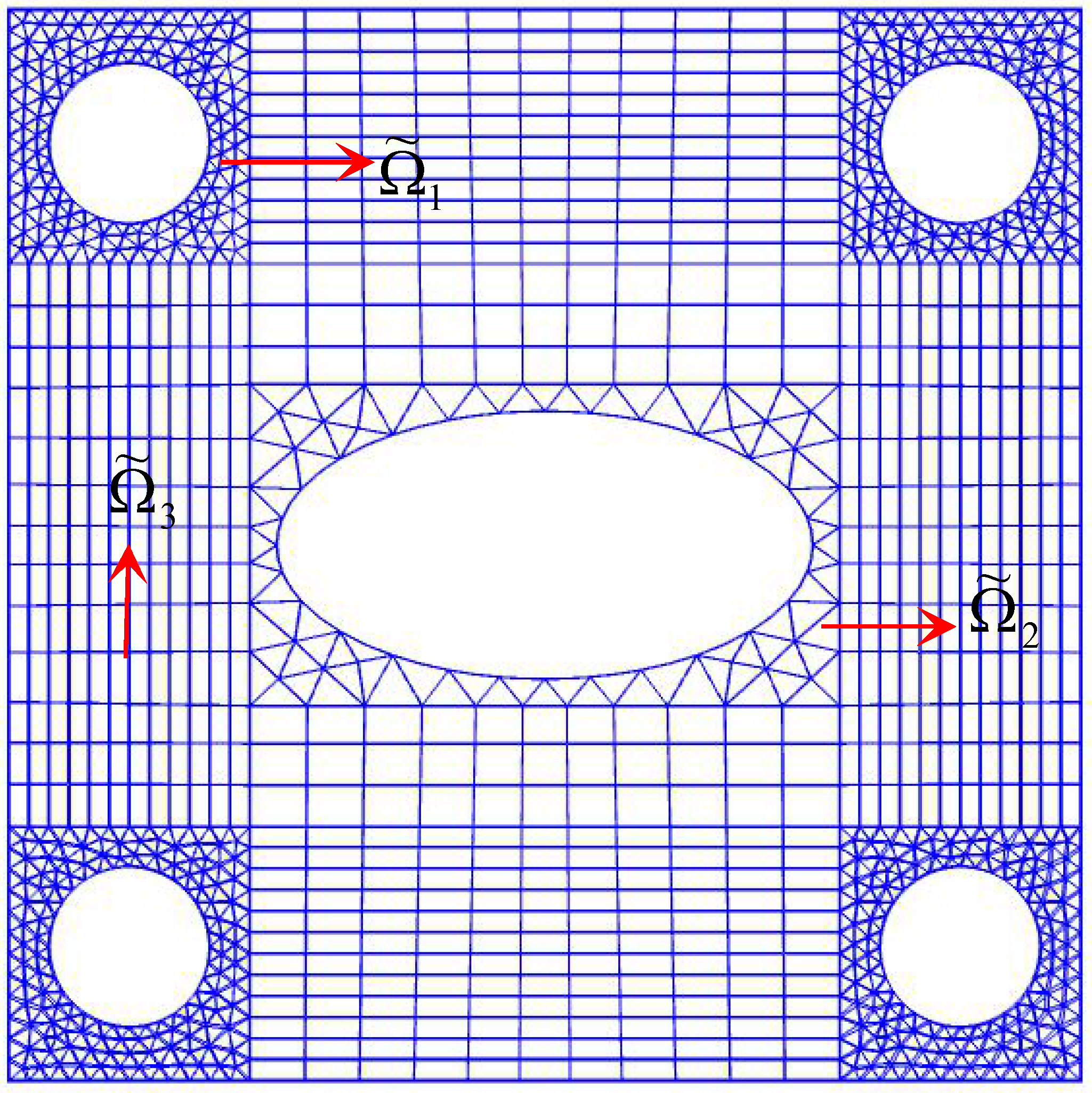
A square thin plate with a hole is shown in Figure 1 below. Four circles with radius R and around the ellipse are wrapped by small rectangles. Four square areas wrapped by small circles are denoted by , one small rectangle wrapped by an ellipse is denoted by , and the other areas are denoted by . The CST element is used for discretization on , the LST element is used for discretization on , and the Q4 element is used for discretization on . Three different types of mesh are common nodes on the junction line of the boundary to ensure that the calculated data can be transmitted to each other.
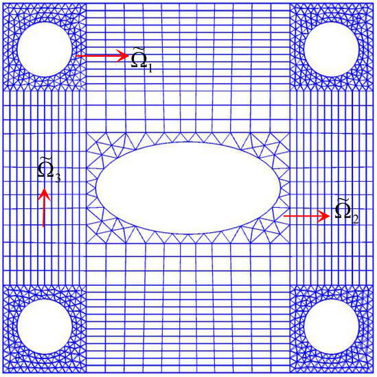
Figure 1.
Hybrid finite element mesh discretization and subregion combination diagram.
There are three different types of meshes in the square plate with holes, and the region division is completed by nesting and combining them with each other. Different subregions are discretized by different element types. In a specific subregion , the displacement component function of any element node (the common node on the boundary line of the non-subregion mesh) can be linearly expressed by the same set of basis functions [28,29]. Because the subregion is of the same element type, its discretization method is similar to the ordinary finite element discretization method. The finite numerical solution corresponding to any coordinate point can be approximated as:
The idea of a weighted basis function is used to approximate the function value of common nodes on the intersection line of subregional grids. If the common nodes on the intersection line of subregional grids contain element types, the corresponding displacement component function approximation value of common nodes on the intersection line can be expressed as Equations (19) and (20):
where is the total number of different sub-mesh types, and the minimum value = 2, indicating that the discrete region of the mixed element is composed of at least two different types of elements. , and represent the number of the CST, LST and Q4 elements, respectively. represents the basis function corresponding to the jth element node in the -th mesh region. is a judgment function of the element node, which is used to determine whether the current node coordinate belongs to the common node in the discrete region, and different subgrid regions are denoted by . Then, each element and vertex of the element in the discrete region is numbered. is the element in the subgrid region when the node coordinate has the corresponding basis function . When the node coordinate has the displacement component function value , the judgment function of the mixed-element sharing nodes is:
In order to facilitate the calculation, all the node coordinates, element number and vertex number in the mesh area are classified and stored. The same type of mesh element is stored in the same set. It should be noted that the common node is the same vertex number in different element types, in order to prevent the error of data information transmission at the common intersection of the mesh in different subregions. The difference between the hybrid element and the traditional finite element is that the basis function of the hybrid element is the basis function combination of multiple different types of elements, while the traditional finite element is the linear combination of the same type of basis function [30,31]. Therefore, the hybrid finite element method is an extension of the traditional finite element method and has stronger flexibility.
Three different subgrid regions correspond to three different cell-based functions. If CST cell-based functions are used in the sub-mesh region, any point of function value on the surface in the subgrid region can be linearly represented by CST cell-based functions. Using isoparametric element transformation, the cell-based functions can be written in vector form, as shown in Equation (22):
The mesh subregion is discretized by a six-node LST element, where . The corresponding basis function is Equation (23):
The Q4 element with four nodes is used for discretization on the mesh subregion , and the corresponding basis function is shown in Equation (24):
Equation (25) is divided into two equations according to the displacement component. If is denoted, there is
Similarly, when , Equation (26) holds:
The continuous calculation region is divided into discrete grid regions, denoted by , with a total of unit vertices and units. The trial function is expressed by linear basis function.
The test function is .
Then, the linear combination of the basis function is substituted into Equation (25) to obtain:
Finally, all the elements in the mesh subregion are assembled to obtain the algebraic equation expression of the first displacement component:
By using the same method, the algebraic equation expression of the second displacement component can be obtained:
The above is mainly for the discrete region , and all subregions have only one type of basis function. For example, the specific subregion uses the CST unit or the LST element. However, there is another case, namely, the type of shared nodes on the intersection of subregions with different unit types [32,33,34]. The derivation of discrete process and weak situation is very similar to Equations (33) and (34). The difference is that only the linear combination of mixed basis functions is used to represent the value of the function to be approximated. We bring the mixed basis functions, as expressed in Equation (27), into the displacement component Equations (31) and (32), respectively. After sorting these out, we can obtain the following two algebraic discrete equations:
The algebraic discrete equation of the second displacement component is:
The numerical solution of the mixed finite element can be obtained by solving the above algebraic equations. Of course, the error and convergence of the approximation of the node function value in the subregion are related to the selected element type, the mesh quality and the order of the basis function, and the convergence will not change within the subregion. The difference is generally on the boundary line of different mesh types. Due to the combination of the mixed basis function, the convergence of the numerical solution at the common node is related to the proportion of the basis function in the approximation term, and the higher the proportion of a specific basis function is. The overall convergence is close to the theoretical convergence order of the basis function type, or it can be considered that the convergence order of the mixed finite element is a linear weighting of the convergence order of multiple basis functions, and the final order depends on the proportion of the basis function in the approximation term [35]. The above is mainly the discrete theory of the mixed finite element. Next, a specific numerical example is given to verify the feasibility of the method.
3. Numerical Example of 2D Thin-Plate Deformation Solved by Hybrid FEM
This numerical example mainly considers a two-dimensional porous elastic plate, and uses the hybrid finite element numerical method to solve the two-dimensional elastic equation. The purpose of this numerical example is to study the advantages of the hybrid finite element in the discretization and numerical solution of special regions. The traditional discrete method of porous thin plate in the regional grid division is to select the triangular element, and the discrete information of the element can be obtained quickly. However, it is not a simple matter to obtain a discrete grid with very high quality. First, the grid division has variability, and it is difficult for a single discrete element to meet the specific requirements. In view of the above problems to be solved, in this paper, a hybrid finite element method is proposed which can effectively improve the grid quality of the calculation area and obtain the numerical solution of the hybrid element [36,37]. The theoretical model given in this paper is equivalent to optimizing the grid structure, and it also expands the application range of the traditional finite element.
In this example, the mixed finite element method is mainly used to solve the deformation problem of the porous elastic plate, and the relevant parameters of the porous elastic plate need to be given. The common structural steel materials are selected in this example, with the Young’s modulus GPa, Poisson ratio v = 0.3, and density . The geometric appearance is mainly a rectangular plate, with four small circular holes and a central elliptical hole inside. The length of the rectangular plate is , and the width is . The center coordinates of the four small circles are and in turn. The radius of the four small circles is . The center elliptical hole long axis , and the short axis . The two-dimensional linear elastic mechanics equation solved by this example is:
The left boundary of the rectangular thin plate is fixed; that is, the displacement boundary condition is:
The right boundary is subjected to vertical downward external force:
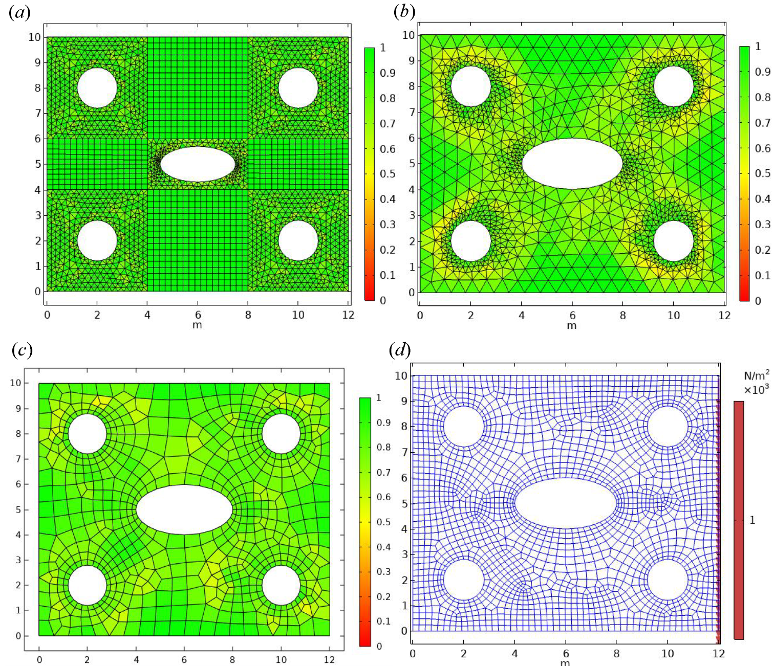
Firstly, the regional grid is divided. In this paper, two different grid division methods are used. One is the hybrid element grid division method, that is, the combination of triangular grid elements and quadrilateral grid elements. The other is the single-grid-type division method, and the discrete element obtained using the single-grid division method has only one type. The grid quality is different in different drawing methods. In this section, the grid quality evaluation formula is given. The results of the two grid divisions are shown in Figure 2.
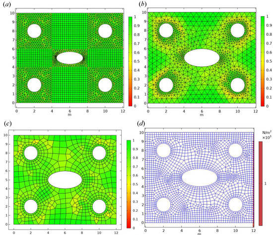
Figure 2.
Comparison of hybrid finite-element mesh and adaptive mesh. (a) Hybrid finite-element mesh quality assessment chart. (b) CST adaptive mesh quality assessment renderings. (c) Q4 adaptive mesh element quality assessment diagram. (d) Schematic diagram of the refined Q4 adaptive mesh and boundary loads.
Mesh quality evaluation can be evaluated from different perspectives, such as area ratio, skewness, maximum angle, condition number, growth rate, circumcircle radius, etc. This example is evaluated according to area ratio, as shown in Equation (38). When the unit is selected as Q4, represents the edge length of any quadrilateral unit, and are the area of the quadrilateral unit, and the best reference object for mesh quality evaluation is the square.
When the unit is CST, , is the area of the triangle unit to be evaluated. When the optimal reference object is an equilateral triangle, is constant. When the optimal reference object is an isosceles right triangle, is constant. The grid quality evaluation formula of the triangle unit is Equation (39):
According to the above method, we can evaluate the two mesh generation methods. The first is the hybrid element grid generation method, which divides the whole solution area into two elements, Q4 and CST. As shown in Figure 2a, the CST element is used near the circular hole, and the Q4 element is used in the other areas. Then, the grid quality is calculated according to the area ratio grid quality evaluation formula for each unit of the region. The closer the mesh quality evaluation result is to 1, the better the grid division effect is, and green is used to show the units in the discrete area. When the mesh quality is closer to 0, which is shown in red color, Figure 2b–d are generated by the second mesh type, and there is only one element type in the solution domain. Figure 2b only uses the CST element for the mesh division, and the division form is combined with the adaptive method. Figure 2c,d only use the Q4 element for the mesh division, and the mesh also has adaptive characteristics when it is close to the circular hole and central ellipse. Then, the mesh quality of each element is calculated. From the effect of mesh quality evaluation, the mesh quality of the mixed-element type is better than that of the single-element type. This also reflects the advantages of hybrid-element combination. Then, the mesh division is equal to the basic information of the calculation. Figure 2a contains 3092 CST elements, with an average quality of . It also contains 918 Q4 elements, with an average quality of , if all the porous elastic plates are discretized by CST elements.
The average mesh quality is , and all the meshes are discretized using Q4 elements, with an average quality of . The hybrid finite element of this example only contains two types of basis functions, namely, CST and Q4. The four circular holes and central ellipses belong to the subregion . In this example, the same CST element is used for discretization. The remaining part belongs to the subregion , and the Q4 element is used for discretization. Therefore, the relationship between the total discrete region and the two subregions can be written as . The purpose of Figure 2 is to compare the grid quality of different element types. It can also be seen from the calculation results that the mesh quality of the hybrid element is better. This comparison is mainly to calculate the average grid quality. For each discrete element in each region, its grid quality is calculated, and then averaged to obtain the average grid quality of the whole region. For Figure 2, there are three cases, namely, the hybrid-element grid, and the adaptive mesh formed by the CST and Q4 elements. In fact, the final comparison is the average mesh quality, which only requires the average mesh size of the element to meet . We believe that these discrete regions are at the same level, and we then compared the average mesh quality so that the comparison results would meet the principle of control variables and in order to ensure the scientific nature of the research method. We performed a comparison of the grid quality at three scales and obtained the same numerical results. This also reflects the rigor of this study.
For the hybrid-element pairs to solve the two-dimensional linear elastic equation, there are mainly two cases. One is that the function value approximation of the nodes in the subregion is similar to that of the traditional finite-element method, because there is only one type of element in the region. At this time, the displacement basis functions of the element in the subregion are shown in Equations (40) and (41):
The second case is that of two different subregional mesh share nodes on the interface connection line. The function value approximation of these points is special, and the common node belongs to the node of the CST element and the Q4 element. Therefore, there are different types of base functions in the approximation terms of these function values. According to this example, there are two kinds of base functions in the approximation terms of the function value of the common node, which can be expressed as:
In Equations (42) and (43), is a hybrid-element node judgment function, selecting node coordinates with hybrid basis functions. Then, according to the mixed-element discrete theory introduced above, the approximation term of the displacement component is introduced into the elastic mechanics equilibrium equation represented by displacement, and the differential equation is transformed into an algebraic equation with an integral term.
Finally, by solving the linear equations, the numerical solution of the displacement component , stress and strain can be obtained. Another feature of this example is the visualization of deformation. Among them, is the initial node coordinate position, is the grid node coordinate after the deformation, and is the deformation factor. The specific calculation formula of displacement numerical solution deformation is shown in the following expression, Equation (44):
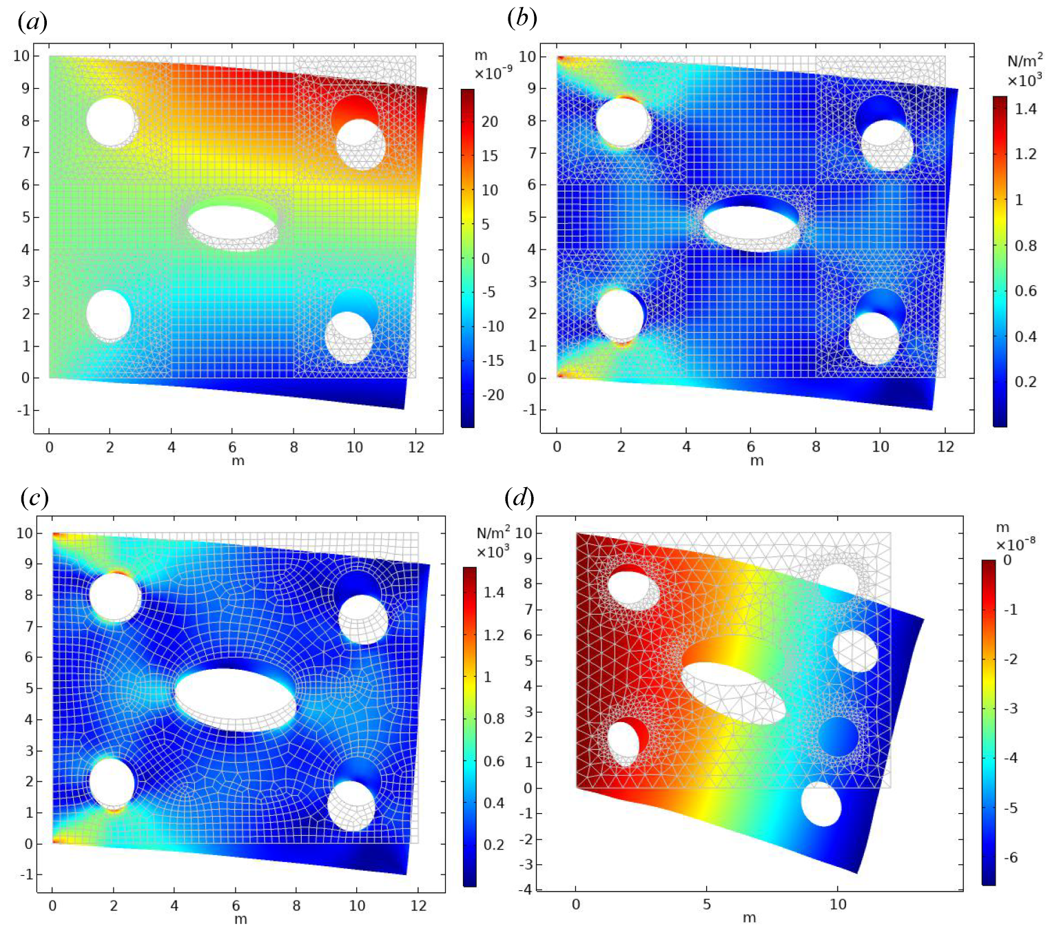
Figure 3 provides the specific numerical solution of mixed elements. Figure 3a is the numerical solution of displacement solved under the mixed-element theory. The white background grid is the original position, and the displacement nephogram of the porous plate with color is the deformation nephogram after deformation. The numerical solution can obviously see that the left fixed is basically unchanged. Because the left end is subjected to the vertical downward force, the downward displacement component U is generated, and the deformation factor . Figure 3b is the numerical solution nephogram of Von Mises stress. The characteristics of this figure are also the results obtained by solving the mixed-element numerical theory. The stress change near the hole is obvious. Another feature of this figure is that the stress diagram is combined with the displacement strain diagram, which can see not only the change in stress but also the change in displacement.
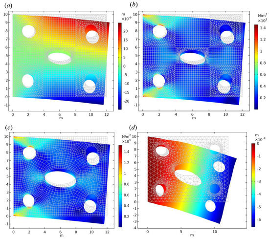
Figure 3.
Numerical results of hybrid finite−element 2D thin−plate deformation. (a) Numerical solution of the hybrid finite-element displacement component U. (b) Numerical solution of Von Mises stress. (c) Von Mises solution of Q4 element adaptive FEM contour diagram of the numerical solution of stress. (d) Schematic diagram of the displacement component V of the CST element adaptive FEM solution.
Figure 3c is the result of a single triangular mesh. The mesh has adaptive characteristics and obvious encryption characteristics near the hole. This figure represents the numerical solution cloud of Von Mises stress, which can be compared with Figure 3b. The stress distribution of the two is basically the same. However, the hybrid element has more advantages in the numerical accuracy of specific regions and the overall solution time. Figure 3d is mainly the grid generated by the quadrilateral element, and the discrete region only contains one CST element. The figure shows the numerical solution cloud of the displacement component V in the y direction. The deformation amplification factor . It can also be seen from the deformation results that when the deformation factor increases, the deformation results are increased.
The numerical results show that the hybrid finite-element method is an extension of the traditional finite-element method; the mesh is also more flexible and can be composed of a variety of mesh types. Different regions choose different element types according to need. In addition, the mesh quality is evaluated according to the formula of mesh element area ratio defined in this chapter. The results show that the quality of the hybrid-element mesh is better than that of the triangular mesh and the structured quadrilateral mesh. From the numerical calculation process, the hybrid finite element has a feature through which the substrate is free to choose, and even the high-order element can be used in the key analysis area. The linear element can be used for the calculation area with relatively flat change, and the mixed approximation idea can be used at the interface nodes, which can greatly balance the calculation efficiency and accuracy.
Therefore, the mixed-element theory has greater advantages for the complex geometric calculation area, realizing the free combination of the mesh type and the basis function type, and greatly expanding the application range of the finite element. However, the analysis of the error and the convergence order is more complex than that of the traditional finite element, because the basis function fixed by the traditional finite element has a stable convergence order and error estimation mode, and the mixed finite element needs a specific analysis of specific problems. Without a fixed error range and convergence order, what can be obtained in the form of the basis function combination is a theoretical reference range. Therefore, the contribution of this paper is to provide specific numerical results and a theoretical analysis in numerical modeling, equation discretization and comparison with the traditional finite element. It can also further extend the mixed-element theory to the three-dimensional case.
It is one-sided to discuss the quality of the numerical method simply from the mesh quality, because the solution of PDE is constantly related to the discrete element quality, and also related to the selection of the basis function and the type of the equation. On the one hand, the hybrid element can realize the free combination of the mesh. Firstly, the discrete quality of each sub-mesh is optimized, and then the average mesh quality of the whole calculation area is optimized. The comparison of the numerical convergence order is to select a numerical method with a faster calculation speed. The total number of discrete elements of the hybrid element is controlled to 0.75–1 times that of the self-use mesh.
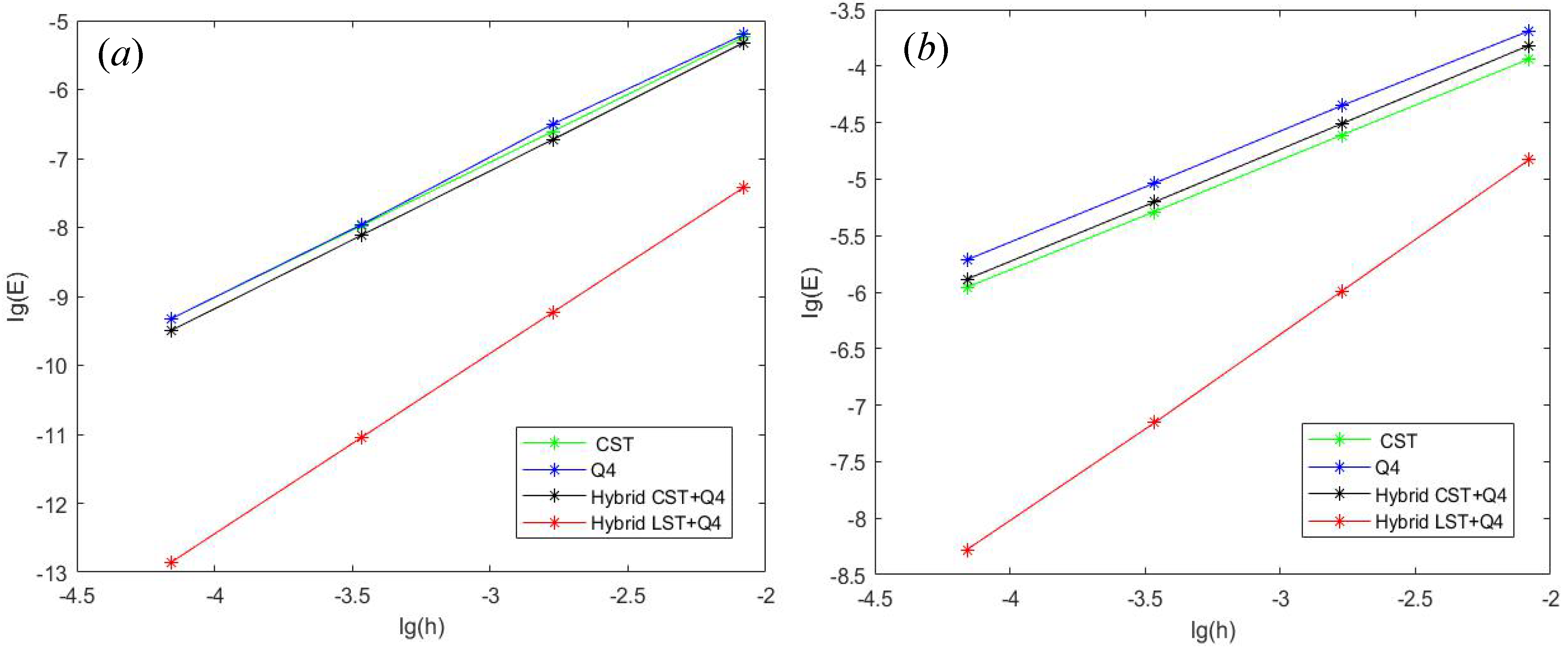
When the number of mixed elements is = 4010 (3092 triangular elements and 918 quadrilaterals), the total number of triangular CST elements is 5012, and the total number of Q4 elements is 4811, the calculation time of = 4 s triangular element is = 4.45 s, and the calculation time of Q4 element is = 4.23 s. However, in terms of convergence rate, the numerical convergence order of displacement is close to order 2. The convergence order of mixed-element displacement using LST + Q4 is about 2.61, and the stress solved by adaptive FEM is about linear convergence. However, the stress convergence order of mixed-element LST + Q4 is close to 1.67. From Figure 4a,b, it can be seen that the convergence speed of the LST + Q4 hybrid element is the fastest. Therefore, when the hybrid element selects the appropriate basis function and good grid combination, the numerical method has the characteristics of short calculation time and fast convergence speed, which also reflects the effectiveness of the method.
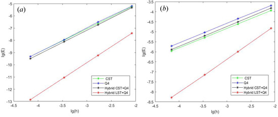
Figure 4.
Hybrid-element numerical convergence comparison diagram (a) displacement numerical convergence comparison diagram (b) Von Mises stress numerical convergence diagram.
4. Simulation and Application of Hybrid FEM in Hydrogen Fuel Battery
4.1. Working Principle of Hydrogen Fuel Battery
Compared with traditional vehicles, the energy conversion efficiency of hydrogen fuel cell vehicles is as high as 60–80%, which is 2∼3 times that of internal combustion engines. The fuel of the hydrogen fuel cell is hydrogen and oxygen and the product is clean water. It does not produce carbon monoxide and carbon dioxide and does not emit sulfur and particulates [38,39]. Therefore, the use of hydrogen energy as the power system of the vehicle can greatly improve the air quality of the city. The electricity generated by a hydrogen fuel cell can be supplied to the motor through inverters, controllers and other devices, and then driven by the transmission system and drive axles to rotate the wheels, so that the vehicle can drive on the road. The electrochemical reaction of hydrogen and oxygen occurs in the stack, and the generated electric energy is driven by the motor. However, in fact, the electrical power that drives the vehicle is not provided directly by the hydrogen fuel cell. In general, the lithium battery pack of the hybrid vehicle is equivalent to power supply.
Hydrogen starts from the anode plate (anode) of the hydrogen fuel cell, and through the catalyst (platinum) in the polymer electrolytic membrane, two electrons in the hydrogen molecule are separated. The hydrogen ions (protons) that lose electrons pass through the proton exchange membrane (the role is to separate hydrogen ions and electrons) and reach the cathode plate (cathode) of the hydrogen fuel cell. However, electrons cannot pass through the proton exchange membrane, and electrons pass through the external circuit to reach the cathode plate of the hydrogen fuel cell, thus generating current in the circuit. After electrons reach the cathode plate, they are recombined with hydrogen ions and oxygen atoms in the air to form water. Because of the oxygen supplied to the cathode plate [40,41], these can be obtained from the air. Therefore, as long as hydrogen is continuously supplied to the anode plate, air is supplied to the cathode plate, water (steam) is taken away in time, and electricity can be continuously provided. Figure 1 presents the application and internal power generation process of the hydrogen fuel cell. The internal structure of the fuel cell is generally composed of five parts, namely, a bipolar plate (metal, graphite, polymer, etc.), an electrode, a catalyst, a proton exchange membrane and an electrolyte solution. The fuel cell hydrogen supply process and internal power generation diagram for new energy vehicles is depicted in Figure 5a, which provides a schematic diagram for adding liquid hydrogen to the new energy vehicle powered by a hydrogen fuel cell. Due to the high cost of production and the difficulty of safety control technology, the current hydrogen fuel cell has not been mass-produced and market-oriented to popularize it to users. In (b), the internal structure and power generation process of a hydrogen fuel cell is depicted, which makes it easier to understand the working principle of hydrogen fuel cells.
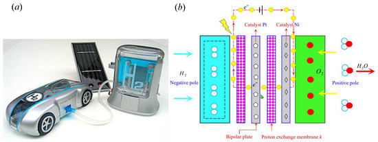
Figure 5.
Application and internal power generation process of hydrogen fuel cells. (a) Schematic diagram of liquid hydrogen for new energy vehicles powered by hydrogen fuel cells. (b) Internal structure and power generation process of hydrogen fuel cells.
4.2. Thermal-Mechanical Coupling Model of Double Electrode Plate
Fuel cells mainly convert the chemical energy of fuel (hydrogen, diesel, methanol and chemical hydride, natural gas) and oxidant (oxygen) into electrical energy through redox reactions [42]. In addition, fuel cells are also called electrochemical batteries. This paper mainly studies hydrogen fuel cells, fuel and oxygen sources (usually from air) to maintain chemical reactions, and in the battery, chemical energy is usually obtained from metals and their ions or oxides that already exist in the battery. As long as fuel and oxygen are available, fuel cells can continuously generate electricity. Electrolytes allow ions (usually hydrogen ion protons with positive charges) to move between the two sides of the fuel cell. At the anode, the catalyst oxidizes the fuel to produce ions (usually positive hydrogen ions) and electrons. Ions move from anode to cathode by electrolyte. At the same time, electrons flow from the anode to the cathode through an external circuit, generating a direct current. In the cathode, another catalyst causes ion, electron and oxygen reactions to form water and other possible products. The start-up time of proton exchange membrane fuel cells (PEMFC) is from 1 s to 10 min. In addition to electricity, fuel cells also produce water and heat according to the fuel source. The energy efficiency of fuel cells is usually between 40 and 60%. However, if waste heat can be combined with thermoelectric materials, up to 85% of the energy utilization rate can be obtained. The fuel cell is subjected to use in the process.
A thermal-mechanical coupled hybrid finite-element model of bipolar plates in a proton exchange membrane fuel cell (PEMFC) is established. The bipolar plates are generally operated at temperatures slightly lower than during the operation of hydrogen fuel cells, which means that additional heating is needed during the start-up process and thermal stress is formed in the bipolar plates after heating. In addition, the many orifices of fuel gas inside the cell are also analyzed. The active component position of the catalyst is also subject to certain pressure. The whole bipolar plate can use thermal-mechanical coupling in a study of the temperature, thermal stress, thermal strain and other physical parameters of the bipolar plate in the continuous power generation process. There is a fuel gas channel at the edge of the bipolar plate, and there is a starting heating element in the middle of the electrode gas feeding channel. Due to the geometric symmetry of the bipolar plate, 1/2 of the actual size of the battery can be considered in the numerical solution.
4.3. Three-Dimensional Steady Heat Conduction
The temperature variable is a multivariate function of space coordinates and time. When is a scalar function controlled by the steady-state heat conduction equation, it means that the temperature of the thermally conducting object does not change with time after heat exchange, which is called the steady-state temperature field. The model of the transient heat conduction equation established in this section (Section 4.3) is related to no time term [43,44]. When is a transient temperature field, the difference between the transient temperature field and the steady temperature field is that there is a time variable t. According to the Fourier heat transfer law and energy conservation law, the heat transfer equation of a battery material plate in a rectangular coordinate system satisfies the following expression.
In this example, the bipolar plate is mainly titanium, and the heat source material with a small circular center is aluminum. In Equation (45), represents different heat transfer coefficients, and is the heat transfer coefficient of in different directions. In this example, it is assumed that the bipolar plate is the isotropic material, and that it satisfies . T represents the temperature of the bipolar plate, and Q represents the heat source. is the density of titanium metal material, and the unit is . Q is the heat generated by the internal heat source, which is often used in the thermal start of the fuel cell [45,46]. Aluminum products are selected because aluminum has good thermal conductivity.
In addition, denotes the heat flux in the and z directions, respectively. The equivalent differential equation of the formula is shown as Equation (46):
In addition, the temperature field function distribution in needs to meet certain boundary conditions.
(1) The first boundary condition:
The solid surface temperature function is a known function about Equation (47):
(2) The second type of boundary conditions:
The heat flux on the solid surface is equal to the sum of the derivative of temperature T along the direction of each component multiplied by the corresponding thermal conductivity, or is called the product of the gradient of temperature and the vector of thermal conductivity. Where = ( ) is the chord of the outer normal direction of the boundary, and is the heat flux on the boundary.
(3) The third boundary condition:
The variation in heat flux on solid surface is equal to the equilibrium value of the surface temperature T and the external temperature after heat exchange. The h in Equation (49) represents the heat exchange coefficient, and the unit is . is the ambient temperature of the boundary layer under convective conditions.
The combination of all boundaries can be expressed as . Then, assuming that the materials used in bipolar plates are all isotropic materials, the thermal conductivity along each component direction is the same; that is, , and thus the convection–diffusion equation can also be written as:
The three-dimensional transient heat conduction Equation (51) is solved. Before being solved, the original problem needs to be transformed into a variational problem, and the variables to be solved are . At the same time, V is an infinite dimensional Banach space denoted by . is a bilinear form marked coincidence, and f is a linear continuous functional. Finding a function makes the variational Equation (51) hold.
Then, the three-dimensional continuous RPV space area is divided into grids, and the divided discrete area is denoted by . After meshing, the data sets such as element number, node number and node coordinates can be obtained. We define the subspace of the finite element as , which is composed of a set of finite dimensional basis functions [47]. is a functional polynomial related to the node of the element, and the finite-element subspace can be abbreviated as . The Galerkin method is used to approximate the problem using the interpolation points of the finite dimension. If the finite-element numerical solution is denoted by , then the finite-element discrete Equation (52) holds.
According to the idea of finite-element approximation, any numerical solution can be linearly represented by the basis function in .
When the common mesh intersects, in Equation (54), represents the judgment function of common nodes, and represents the number of nodes of the ith type of mesh element.
Finally, the linear approximation term of the mixed finite element is substituted into the weak situation equation, and the algebraic equation with an integral form can be obtained. Combined with the boundary treatment, a sparse linear equation group can be obtained. If it is a steady-state heat conduction equation, it can directly solve a linear equation group. However, for the transient heat conduction equation, the time term containing the time term needs to be discreted by combining it with the finite difference. Finally, it can be transformed into an iterative formula, and the final numerical solution can be obtained by combining it with the initial value. Finally, the numerical solution of the three-dimensional temperature function is visualized, and the change of temperature at different times can be observed. According to the above theory, the variational form of the original problem is obtained.
Combined with the Galerkin approximation principle, a basis function is selected in the finite-element subspace to discretize the equation:
Combining Equation (54) and considering the right-hand term of the heat source, the variational form of the heat conduction differential equation can be obtained, and Equation (57) can be obtained after simplification.
Then, the temperature function T is replaced by the approximate solution of the finite element.
Then, considering the second kind of boundary and the third kind of boundary conditions, the weak situation of Galerkin can be obtained through Equation (59):
We set the stiffness matrix and the right-hand term corresponding to the heat conduction equation on any element, and then the linear equation on the element is .
The solution space of the mixed finite element is composed of many different types of elements. In this example, the tetrahedral and hexahedral elements are used for discretization, and the dimension of the element matrix is equal to . Therefore, the dimension of the tetrahedral is , and the dimension of the hexahedral is . The corresponding linear discrete equation on each element is:
The single rigid matrix is assembled to form the whole linear equation group. represents the number of elements divided by in the bipolar plate region of the whole fuel cell. represents the total number of tetrahedral units in the region. represents the total number of hexahedral units. The corresponding results of the total linear equation formed by the single rigid matrix assembly are as follows:
Finally, we can represent the node temperature function values at any point on the discrete domain as follows:
In addition, certain thermal stress and thermal strain are also formed in the long-term high-temperature environment [48,49]. It is assumed that the distribution of temperature difference in the bipolar plate is denoted by , and the expansion coefficient is denoted by . The physical equation considering thermal expansion can be written as:
Finally, the thermal stress matrix can be expressed as:
The thermal strain is recorded as:
4.4. Three-Dimensional Static Elastic Equation
When the fuel cell works, it also receives the thermal stress , the gas passes through the active material pressure , and the impact pressure of the exhaust gas passes through the manifold outlet [50]. When these forces are applied to the bipolar plate of the fuel cell, the bipolar plate also deforms. The hybrid finite-element method proposed in this paper can be used to solve the stress, strain, displacement and other physical quantities of the bipolar plate. These physical quantities can be obtained according to the three-dimensional linear elastic equation. The static three-dimensional linear elastic equation is as follows:
In the above formula, is the volume external force, is the stress tensor, is the three-dimensional gradient operator, and is the divergence of the stress tensor. The three-dimensional static elastic equation can also be expressed as . The three-dimensional displacement field function can be expressed as , and represents the number of two element nodes, respectively. The mixed finite-element approximation base function of displacement can be written as:
In terms of the representation of the basis function of the hybrid finite element, represents the grid type judgment function, and represents two types of grids, which also indicates that the discrete region of this example is composed of two types of elements. When represents the common boundary region of the grid, it is represented by two kinds of basis function.
Then, the Galerkin method is used to discrete the linear elastic equation. The discrete region is denoted by . If the finite-element solution of the displacement function is , a test function is selected as .
By using Gauss divergence theorem and the divergence term of stress tensor, it can be deduced that
Then, by using the divergence theorem, the first integral term of the right end term is converted to an area fraction.
In the formula, represents the unit normal vector of the solution domain boundary pointing to the inside, and S is the surface of the boundary region. Combined with Equation (79), we can obtain:
where is the boundary surface force, the Galerkin form of the three displacement component equations is:
For the stress terms in Equations (82)–(84), the displacement function can be used to replace them, and the specific formula is . The corresponding elastic matrix is shown in Equation (85):
The three-dimensional strain can be obtained according to the geometric equation. The vector of strain expressed by displacement can be written as follows:
For the mesh subregion of the same element type, denoted by , the stress function of any node can be written as follows:
Another unit basis function of the fuel cell bipolar plate is denoted by , and the stress function can be expressed as:
For the approximation of the mixed-element stress function, it can be expressed as:
Similarly, other mixed-element approximations of stress are written as follows:
4.5. Material Parameter Setting of Numerical Calculation
The main solution of the numerical example is the bipolar plate of the fuel cell plate. The numerical example is based on the thermal-mechanical coupling model established using the mixed finite-element method [51,52]. The plate will have heat inside the plate when it is working normally, forcing the existence of thermal stress in the bipolar plate. The ventilation channel at the edge of the bipolar plate will also be subject to some manifold pressure , and the active components will also be subject to pressure . The center of the bipolar plate has a heating aluminum device. The geometric parameters and material parameters of the bipolar plate are shown in Table 1.

Table 1.
Classification of nuclear pressure vessels by temperature and pressure.
4.6. Numerical Results
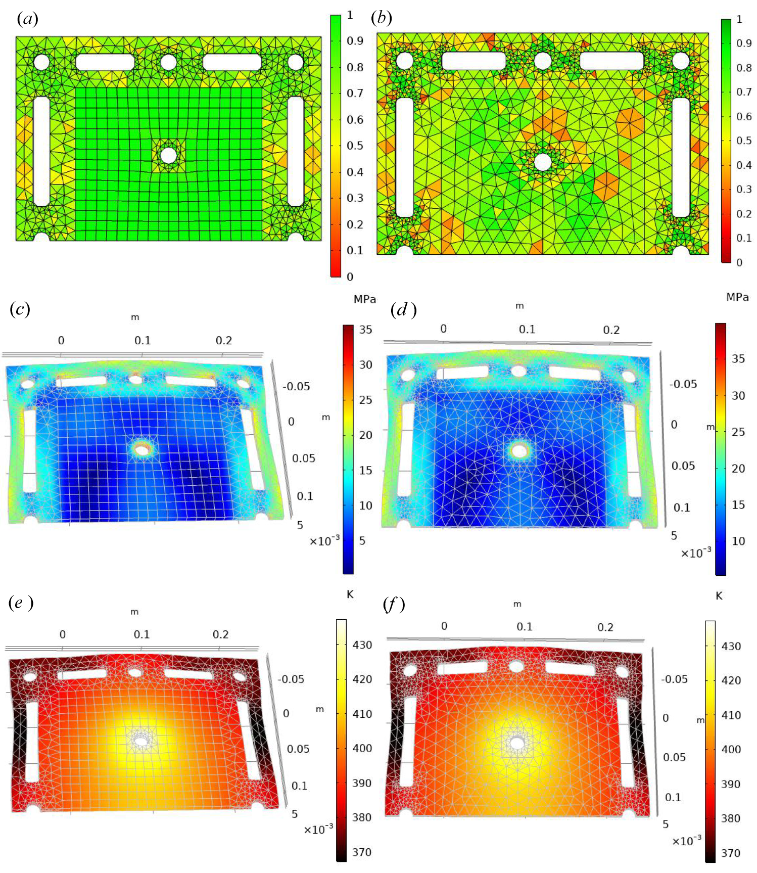
The hybrid finite thermo-mechanical coupling model established in this paper was used to solve the bipolar plate, which is mainly to solve the three-dimensional steady-state heat conduction equation and the three-dimensional static linear elastic equation. The surrounding of the bipolar plate was the channel of the fuel gas, and the center was the aluminum heated circular plate. The solution region of hydrogen fuel cell bipolar plate is a multi-connected rectangular region. Figure 6 is the numerical solution of the hybrid element of the fuel cell. Figure 6a,b are mainly the comparison results of the two types of mesh quality. (a) The number of hexahedral elements was 258, the number of tetrahedral elements was 534 and the number of mesh vertices was 2030. The average mesh quality was 0.82. (b) There were 1794 tetrahedral elements, and there were 2919 mesh vertices at the mesh vertices. The average mesh quality was 0.68. The comparison of the two images shows that the mesh quality of the mixed element was higher, and the common feature was that the mesh quality at the edge of the bipolar plate was relatively poor.
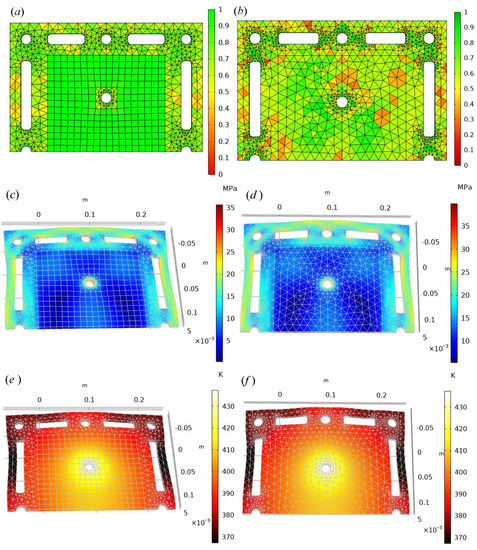
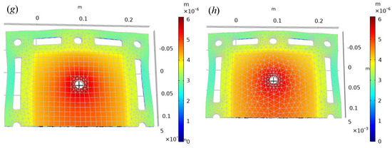
Figure 6.
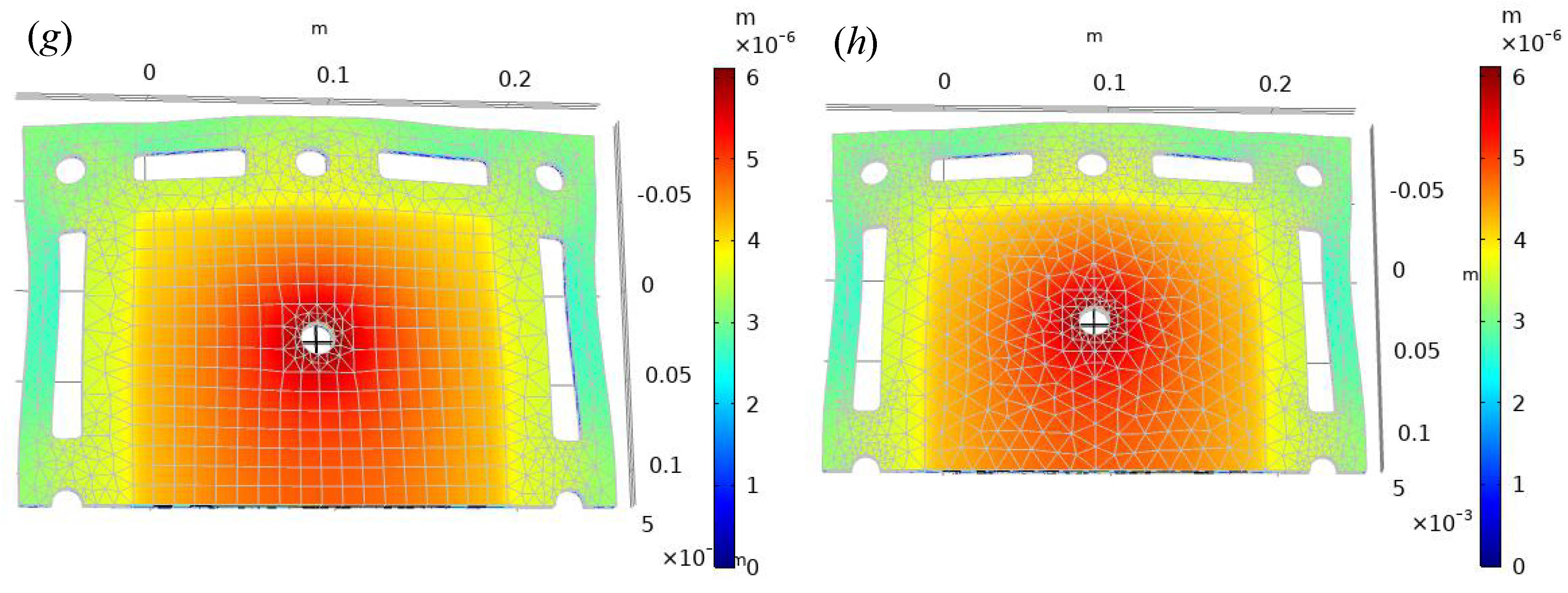
The comparison between the numerical solution of the thermo-mechanical coupling model of the hybrid finite element corresponding to the bipolar fuel cell plate and the adaptive FEM. (a) Hybrid−element grid quality assessment results. (b) Adaptive FEM grid quality assessment results. (c) Von Mises stress diagram of hybrid finite element. (d) Von Mises stress diagram solved using adaptive FEM. (e) Temperature T nephogram of hybrid finite element. (f) Temperature T numerical solution nephogram solved using adaptive FEM. (g) Displacement nephogram . (h) Displacement value solution nephogram solved using adaptive FEM.
The same feature is that the quality of the grid at the edge of the bipolar plate vent was relatively poor. Of course, we can also compare various numerical stresses, such as the thermal stress tensor . When the equivalent stress and strain at a certain point reached a certain value related to the stress and strain state, the material yielded. In other words, when the material was in a plastic state, the equivalent stress was always a constant value. This example mainly compares the Von Mises stresses. Figure 6c is the Von Mises stress solved using the mixed finite element method. The larger stress values concentrated on the edge and the center round hole. Figure 6d shows that the numerical results of the two adaptive FEM figures were basically the same, and the positions of the maximum and minimum distributions were consistent with the mixed-element numerical solutions. The purpose of this numerical experiment is to observe the amount of information such as thermal−stress, thermal−strain, and displacement of the fuel bipolar plate when the fuel cell is at high temperature and under the action of fuel gas. Another feature of this paper is that the deformation of the bipolar plate can be simulated. According to the displacement change, combined with the deformation factor, the deformation variables are appropriately amplified, so that it is more convenient to compare the position of the displacement change and the change of thermal−stress. This information is very important in the design of the internal structure of the fuel cell, because unreasonable design will cause the internal heat to be unable to dissipate in time. Secondly, serious deformation will also affect the power generation efficiency and battery life. These problems reflect the research value of this paper.
Figure 6e is the numerical solution of the temperature of the mixed element. This temperature is mainly the radiation of the central heat source to the surrounding area, and the temperature decreases point by point. The edge temperature was close to 370 K, and the central temperature was close to 420 K. Figure 6e is the numerical solution of the mixed element, and Figure 6f is the numerical solution of the adaptive FEM. The temperature distribution of the steady state of the three questions can be solved according to the heat conduction equation, and the temperature also causes information such as thermal stress and thermal strain. Figure 6g is the numerical solution of the displacement of the mixed finite element W. The variation at the center of the displacement was relatively large, because there was a self-heater of aluminum products in the center. As a result, the center temperature was high and the expansion ratio was serious. Therefore, the displacement value changed relatively significantly. Figure 6h is the corresponding cloud image of the displacement numerical solution W of the adaptive FEM. Compared with Figure 6g, the same phenomenon was found. The central displacement changed greatly, and the order of magnitude of the displacement was .
Through the comparison of the above numerical solutions, not only was the hybrid finite element found to have a high mesh quality, but also the numerical solution results were highly consistent with the adaptive numerical solution. The hybrid finite element could use fewer elements in the total number of grid elements. The displacement convergence speed of the hybrid element was faster than that of the adaptive finite element, which was close to second-order convergence. The convergence speed of the adaptive finite element was slightly lower, which was close to 1.86–1.92. The speed of the hybrid finite element was faster than that of the adaptive finite element. Under the condition of good mesh segmentation, the hybrid element only needed about 4.1 s time. However, the solution time of the adaptive FEM was close to 6.5 s. The above numerical results show that the hybrid finite-element method has more advantages in solving the thermal-mechanical coupling problem. Especially for the multi-connected region, the hybrid element is more flexible, and different regions can be discreted by different element types. The hybrid finite-element method has a better grid quality and a higher convergence rate than the traditional adaptive method, and the number of elements required is relatively small, which also improves the solution time. Of course, the defect in the hybrid element is that the grid division requires some prior knowledge, and the free matching problem of the mesh needs to be completed according to the actual needs.
5. Conclusions
In this paper, a hybrid-element method was proposed to solve the thermal-mechanical coupling model of the fuel cell plate, which can effectively solve the thermal stress change, temperature field distribution and displacement change in the fuel cell plate at work. In this paper, the hybrid-element algorithm for the deformation of a 2D plate was given first, and then the deformation application of a 3D fuel cell plate was given. This paper mainly studied the deformation problem of a porous elastic plate. In view of the defects of the traditional method, such as the poor quality of discrete grids, the low efficiency of numerical calculation and the difficulty in the local adjustment of calculation area, etc., in this paper, an efficient hybrid finite-element numerical method was proposed. The hybrid finite-element solution theory was given for the deformation of porous elastic plates. Compared with the traditional CST adaptive finite-element method and Q4 adaptive finite-element method, the hybrid finite-element method is more flexible for realizing the flexible combination of the grid and the finite-element basis function. This paper also provided a new formula for the evaluation of grid quality, which can effectively evaluate the mesh quality of triangular and quadrilateral elements. For the grid quality evaluation of the hybrid element, the average method was used in this paper. From the numerical experiment results, it can be seen that the mesh quality of the hybrid element was significantly higher than that of the traditional CST and Q4 adaptive mesh. Another advantage of the hybrid element is that the refined mesh can be realized for the key areas, and the order of the basis function can also be adjusted according to the actual needs.
Therefore, this method realizes the balance between numerical accuracy and solution efficiency, especially for the local porous elastic plate problem. The hybrid-element method is obviously superior to the traditional method. The hybrid element can use fewer elements to achieve rapid convergence, and the method proposed in this paper is obviously adaptive FEM convergence fast. In addition, this paper also gives the deformation control formula, which can display the displacement deformation and stress combined diagram on the graphics at the same time, which is convenient to quickly compare the regions where the displacement and stress extremum appear. In short, this paper provides a good foundation for the expansion of the finite-element numerical method, and can provide a mechanical model reference for solving the mechanical problems of porous elastic plates and complex topological geometric regions. Finally, the three-dimensional numerical results were similar to the two-dimensional results; that is, the hybrid finite-element numerical method realized the free combination of the mesh and the basis function, and could form a higher grid quality. In addition, the numerical convergence rate was more advantageous. In this paper, the discrete theory of 2D and 3D problems was provided. These are an extension of the traditional FEM method and an interdisciplinary application case. The hybrid finite element has more applications and further applications to be found. For example, it is still a very difficult scientific research problem to expand toward crack and discontinuous problems with defects. However, it is also a very valuable algorithm innovation and has broad application prospects.
Author Contributions
Conceptualization, W.C., S.D. and B.Z.; methodology and experiments, W.C.; writing—original draft preparation, W.C.; writing—review and editing, W.C., B.Z and S.D.; visualization, W.C.; supervision, B.Z. and S.D.; funding acquisition, S.D. All authors have read and agreed to the published version of the manuscript.
Funding
This work is supported by the Young Science Foundation CN (No.11701433), Technology Major Project of Hubei Province under Grant 2021AAA010, and by the National Natural Science Foundation of China (Grant No. 12071363).
Institutional Review Board Statement
Not applicable.
Informed Consent Statement
Informed consent was obtained from all subjects involved in the study.
Data Availability Statement
Data for this article can be accessed publicly.
Acknowledgments
We would like to thank the anonymous reviewers for professional advice.
Conflicts of Interest
The authors declare that they have no known competing financial interests or personal relationships that could have appeared to influence the work reported in this paper.
References
- Li, Y.; Taghizadeh-Hesary, F. The economic feasibility of green hydrogen and fuel cell electric vehicles for road transport in China. Energy Policy 2022, 160, 112703. [Google Scholar] [CrossRef]
- Wu, Y.; Liu, F.; He, J.; Wu, M.; Ke, Y. Obstacle identification, analysis and solutions of hydrogen fuel cell vehicles for application in China under the carbon neutrality target. Energy Policy 2021, 159, 112643. [Google Scholar] [CrossRef]
- Yu, S.S.; Lee, T.H.; Oh, T.H. Ag–Ni nanoparticles supported on multiwalled carbon nanotubes as a cathode electrocatalyst for direct borohydride–hydrogen peroxide fuel cells. Fuel 2022, 315, 123151. [Google Scholar] [CrossRef]
- Shen, Y.; Yan, X.; An, L.; Shen, S.; An, L.; Zhang, J. Portable proton exchange membrane fuel cell using polyoxometalates as multi-functional hydrogen carrier. Appl. Energy 2022, 313, 118781. [Google Scholar] [CrossRef]
- D’Angelo, C.; Scotti, A. A mixed finite element method for Darcy flow in fractured porous media with non-matching grids. Math. Model. Numer. Anal. 2012, 46, 465–489. [Google Scholar] [CrossRef] [Green Version]
- Cattaneo, L.; Formaggia, L.; Iori, G.; Scotti, A.; Zunino, P. Stabilized extended finite elements for the approximation of saddle point problems with unfitted interfaces. Calcolo 2015, 52, 123–152. [Google Scholar] [CrossRef]
- Hansbo, P.; Larson, M.; Zahedi, S. A cut finite element method for a Stokes interface problem. Appl. Numer. Math. 2014, 85, 90–114. [Google Scholar] [CrossRef] [Green Version]
- Sacco, R.; Mauri, N.G.; Guidoboni, G. A stabilized dual mixed hybrid finite element method with Lagrange multiplicrs for three-dimensional problems with internal interfaces. J. Sci. Comput. 2020, 82, 60. [Google Scholar] [CrossRef]
- Cao, P.; Chen, J.; Wang, F. An extended mixed finite element method for elliptic interface problems. Comput. Math. Appl. 2022, 113, 148–159. [Google Scholar] [CrossRef]
- Sukontasukkul, P.; Panklum, K.; Maho, B.; Banthia, N.; Jongvivatsakul, P.; Imjai, T.; Sata, V.; Limkatanyu, S.; Chindaprasirt, P. Effect of synthetic microfiber and viscosity modifier agent on layer deformation, viscosity, and open time of cement mortar for 3D printing application. Constr. Build. Mater. 2022, 319, 126111. [Google Scholar] [CrossRef]
- Choi, J.; Choi, B.; Heo, S.; Oh, Y.; Shin, S. Numerical modeling of the thermal deformation during stamping process of an automotive body part. Appl. Therm. Eng. 2018, 128, 159–172. [Google Scholar] [CrossRef]
- Ying, B.; Liu, X. Skin-like hydrogel devices for wearable sensing, soft robotics and beyond. iScience 2021, 24, 103174. [Google Scholar] [CrossRef] [PubMed]
- Meduri, S.; Cremonesi, M.; Frangi, A.; Perego, U. A Lagrangian fluidstructure interaction approach for the simulation of airbag deployment. Finite Elem. Anal. Des. 2022, 198, 103659. [Google Scholar] [CrossRef]
- Chen, W.; Dai, S.; Zheng, B. ARIMA-FEM Method with Prediction Function to Solve the Stress-Strain of Perforated Elastic Metal Plates. Metals 2022, 12, 179. [Google Scholar] [CrossRef]
- Ponta, F.L.; Otero, A.D.; Lago, L.I.; Rajan, A. Effects of rotor deformation in wind-turbine performance: The Dynamic Rotor Deformation Blade Element Momentum model (DRDBEM). Renew. Energy 2016, 92, 157–170. [Google Scholar] [CrossRef] [Green Version]
- Uomoto, T.; Satoh, K.; Okada, H.; Yusa, Y. Mesh-independent data point finite element method (MDP-FEM) for large deformation elastic-plastic problems—An application to the problems of diffused necking. Finite Elem. Anal. Des. 2017, 136, 18–36. [Google Scholar] [CrossRef]
- Dezfooli, M.S.; Khoshghalb, A.; Shafee, A. An Automatic Adaptive Edge-based Smoothed Point Interpolation Method for Coupled Flow-Deformation Analysis of Saturated Porous Media. Comput. Geotech. 2022, 145, 104672. [Google Scholar] [CrossRef]
- Östby, J.; Toller-Nordström, L.; Norgren, S. Insights into plastic deformation and binder lamella orientation in hardmetal turning inserts. Int. J. Refract. Met. Hard Mater. 2022, 103, 105779. [Google Scholar] [CrossRef]
- Huang, L.; Zhang, B.; Shi, Y. Def3D, a FEM simulation tool for computing deformation near active faults and volcanic centers. Phys. Earth Planet. Inter. 2020, 309, 106601. [Google Scholar] [CrossRef]
- Dudek, M.; Tajdu, K. FEM for prediction of surface deformations induced by flooding of steeply inclined mining seams. Geomech. Energy Environ. 2021, 28, 100254. [Google Scholar] [CrossRef]
- Varandas, J.N.; Paixão, A.; Fortunato, E.; Coelho, B.Z.; Hölscher, P. Long-term deformation of railway tracks considering train-track interaction and non-linear resilient behaviour of aggregates a 3D FEM implementation. Comput. Geotech. 2020, 126, 103712. [Google Scholar] [CrossRef]
- Chen, W.; Dai, S.; Zheng, B.; Lin, H. An Efficient Evaluation Method for Automobile Shells Design Based on Semi-supervised Machine Learning Strategy. J. Phys. Conf. Ser. ICCBD2021 2022, 2171, 012026. [Google Scholar] [CrossRef]
- Odermatt, A.; Richert, C.; Huber, N. Prediction of elastic-plastic deformation of nanoporous metals by FEM beam modeling: A bottom-up approach from ligaments to real microstructures. Mater. Sci. Eng. A 2020, 791, 139700. [Google Scholar] [CrossRef]
- Zhou, L.; Yang, H.; Ma, L.; Zhang, S.; Li, X.; Ren, S.; Li, M. On the static analysis of inhomogeneous magnetoelectro-elastic plates in thermal environment via element free Galerkin method. Eng. Anal. Bound. Elem. 2022, 134, 539–552. [Google Scholar] [CrossRef]
- Silveira, T.D.; Baumgardt, G.R.; Rocha, L.A.O.; Santos, E.D.; Isoldi, L.A. Numerical simulation and constructal design applied to biaxial elastic buckling of plates of composite material used in naval structures. Compos. Struct. 2022, 290, 115503. [Google Scholar] [CrossRef]
- Chai, Y.; Du, S.; Li, F.; Zhang, C. Vibration characteristics of simply supported pyramidal lattice sandwich plates on elastic foundation: Theory and experiments. Thin-Walled Struct. 2021, 166, 108116. [Google Scholar] [CrossRef]
- Fu, G.; Yang, Y. A hybrid-mixed finite element method for single-phase Darcy flow in fractured porous media. Adv. Water Resour. 2022, 161, 104129. [Google Scholar] [CrossRef]
- Wan, Y.; Wu, N.; Chen, Q.; Li, W.; Hu, G.; Huang, L.; Ouyang, W. Coupled thermal hydrodynamic mechanicalchemical numerical simulation for gas production from hydrate bearing sediments based on hybrid finite volume and finite element method. Comput. Geotech. 2022, 145, 104692. [Google Scholar] [CrossRef]
- Su, J.; Zheng, L. Smooth finite element construction and correction method based on hybrid FE-SEA model. Appl. Acoust. 2022, 188, 108541. [Google Scholar] [CrossRef]
- Sun, Y.; Chen, B.; Edwards, M.G.; Li, C. Investigation of hydraulic fracture branching in porous media with a hybrid finite element and peridynamic approach. Theor. Appl. Fract. Mech. 2021, 116, 103133. [Google Scholar] [CrossRef]
- Chen, X.; Gong, C.; Liu, J.; Pang, Y.; Deng, L.; Chi, L.; Li, K. A novel neural network approach for airfoil mesh quality evaluation. J. Parallel Distrib. Comput. 2022, 164, 123–132. [Google Scholar] [CrossRef]
- Xie, K.; Jin, Y.; Peng, Y.; Liu, G.; Wan, B. Research on high quality mesh method of armored umbilical cable for deep sea equipment. Ocean. Eng. 2021, 221, 108550. [Google Scholar] [CrossRef]
- Li, S.; Wu, Y. Energy-preserving mixed finite element methods for the elastic wave equation. Appl. Math. Comput. 2022, 422, 126963. [Google Scholar] [CrossRef]
- Zhang, J.; Han, H.; Yu, Y.; Liu, J. A new two-grid mixed finite element analysis of semi-linear reaction–diffusion equation. Comput. Math. Appl. 2021, 92, 172–179. [Google Scholar] [CrossRef]
- Chen, J.; Wang, F.; Chen, H. Probability-conservative simulation for Lévy financial model by a mixed finite element method. Comput. Math. Appl. 2022, 106, 92–105. [Google Scholar] [CrossRef]
- Yu, N.; Li, R.; Kong, W.; Gao, L.; Wu, X.; Wang, E. A hybrid grid-based finite-element approach for three-dimensional magnetotelluric forward modeling in general anisotropic media. Comput. Geosci. 2022, 159, 105035. [Google Scholar] [CrossRef]
- Gao, X.; Xu, S.; Tang, W. Hybrid analytic-FEM approach for dynamic response analysis of air-cushion vehicle skirts. Mar. Struct. 2021, 79, 103062. [Google Scholar] [CrossRef]
- Jafari, H.; Safarzadeh, S.; Azad-Farsani, E. Effects of governmental policies on energy-efficiency improvement of hydrogen fuel cell cars: A game-theoretic approach. Energy 2022, 254, 124394. [Google Scholar] [CrossRef]
- Lee, Y.; Lee, M.C.; Kim, Y.J. Barriers and strategies of hydrogen fuel cell power generation based on expert survey in South Korea. Int. J. Hydrogen Energy 2022, 47, 5709–5719. [Google Scholar] [CrossRef]
- Kar, S.K.; Bansal, R.; Harichandan, S. An empirical study on intention to use hydrogen fuel cell vehicles in India. Int. J. Hydrogen Energy 2022, 47, 46, 19999–20015. [Google Scholar] [CrossRef]
- Scott, K. 4.01—Introduction to Hydrogen, Electrolyzers and Fuel Cells Science and Technology. In Comprehensive Renewable Energy, 2nd ed.; Letcher, T.M., Ed.; Elsevier: Amsterdam, The Netherlands, 2022; pp. 1–28. [Google Scholar]
- Sürer, M.G.; Arat, H.T. Advancements and current technologies on hydrogen fuel cell applications for marine vehicles. Int. J. Hydrogen Energy 2022, 47, 19865–19875. [Google Scholar] [CrossRef]
- Qin, M.; Huo, Y.; Han, G.; Yue, J.; Zhou, X.; Feng, Y.; Feng, W. Three-dimensional boron nitride network/polyvinyl alcohol composite hydrogel with solid–liquid interpenetrating heat conduction network for thermal management. J. Mater. Sci. Technol. 2022, 127, 183–191. [Google Scholar] [CrossRef]
- Chen, W.; Dai, S.; Zheng, B. A Dynamic Thermal-Mechanical Coupling Numerical Model to Solve the Deformation and Thermal Diffusion of Plates. Micromachines 2022, 13, 753. [Google Scholar] [CrossRef] [PubMed]
- Wu, Q.; Peng, M.J.; Fu, Y.D.; Cheng, Y.M. The dimension splitting interpolating element-free Galerkin method for solving three-dimensional transient heat conduction problems. Eng. Anal. Bound. Elem. 2021, 128, 326–341. [Google Scholar] [CrossRef]
- Shiah, Y.C.; Chang, R.Y.; Hematiyan, M.R. Three-dimensional analysis of heat conduction in anisotropic composites with thin adhesive/interstitial media by the boundary element method. Eng. Anal. Bound. Elem. 2021, 123, 36–47. [Google Scholar] [CrossRef]
- Pan, W.; Li, H.; Wang, M.; Wang, L. Elastothermodynamic damping modeling of three-layer Kirchhoff–Love microplate considering three-dimensional heat conduction. Appl. Math. Model. 2021, 89, 1912–1931. [Google Scholar] [CrossRef]
- Liu, Z.; Huang, L.; Liang, J.; Wu, C. A three-dimensional indirect boundary integral equation method for modeling elastic wave scattering in a layered half-space. Int. J. Solids Struct. 2019, 169, 81–94. [Google Scholar] [CrossRef]
- Matsumoto, E.; Hase, T.; Suzuki, T. Three-dimensional constitutive equations of ferromagnetic materials with magnetoelastic coupling: Determination of elastic coefficients under magnetic field. J. Mater. Process. Technol. 2007, 181, 165–171. [Google Scholar] [CrossRef]
- Chen, W.; Dai, S.; Zheng, B. Continuum Damage Dynamic Model Combined with Transient Elastic Equation and Heat Conduction Equation to Solve RPV Stress. Fractal Fract. 2022, 6, 215. [Google Scholar] [CrossRef]
- Liu, X.Q.; Cao, L.Q.; Zhu, Q.D. Multiscale algorithm with high accuracy for the elastic equations in three-dimensional honeycomb structures. J. Comput. Appl. Math. 2009, 233, 905–921. [Google Scholar] [CrossRef]
- Zakharov, D.D. Asymptotic analysis of three-dimensional dynamical elastic equations for a thin multilayer anisotropic plate of arbitrary structure. J. Appl. Math. Mech. 1992, 56, 637–644. [Google Scholar] [CrossRef]

Publisher’s Note: MDPI stays neutral with regard to jurisdictional claims in published maps and institutional affiliations. |
© 2022 by the authors. Licensee MDPI, Basel, Switzerland. This article is an open access article distributed under the terms and conditions of the Creative Commons Attribution (CC BY) license (https://creativecommons.org/licenses/by/4.0/).